Novel Geometrical Models of Relativistic Stars.
II. Incompressible Stars and Heavy Black Dwarfs

Abstract

In a series of articles we describe a novel class of geometrical models of relativistic stars. Our approach to the static spherically symmetric solutions of Einstein equations is based on a careful physical analysis of radial gauge conditions.

It turns out that there exist heavy black dwarfs: relativistic stars with arbitrary large mass, which are to have arbitrary small radius and arbitrary small luminosity. In the present article we mathematically prove this new phenomena, using a detailed consideration of incompressible GR stars. We study the whole two parameter family of solutions of extended TOV equations for incompressible stars. This example is used to illustrate most of the basic features of the new geometrical models of relativistic stars. Comparison with newest observational data is discussed.

PACS number(s): 04.20.Cv, 04.20.Jb, 04.20.Dw

I Introduction

This is the second of series articles in which we describe a new geometrical models of general relativistic stars (GRS). One can find the general scheme, notations, basic equations, additional conditions and basic principles and properties of these models in the first article of this series – F04NMGS . The essentially new features of GRS in these new models are not based on the critics or revision of very general relativity (GR). They are a result of more deep understanding of its applications, and on solution of some open problems in this theory, like the physical justification of the choice of GR gauges. The preliminary knowledge of the article F04NMGS is highly recommended. It is essential for the right understanding of the present one.

Here we consider the simplest specific example of application of the general scheme, described in F04NMGS : GRS, made of an incompressible matter with equation of state (EOS):

$$\varepsilon(p)=const=\varepsilon.$$ (I.1)

In Eq. (I.1) $\varepsilon$ is the energy density and $p$ is the pressure of stelar matter. We are using units $c=G_{N}=1$. Further on the letter $"C"$, as an index of different quantities, denotes their values at the center of the star, the sign $"*"$ – the values at the edge of the star.

Such simple model has a limited physical significance, because it leads to an infinite speed of the sound in the fluid books . Nevertheless, its consideration is useful, because:

$\bullet$ It gives some general estimations for the properties of the solutions of extended Tolman-Openheimer-Volkov (ETOV) equations with arbitrary EOS books .

$\bullet$ This simple model can be used as a good physical approximation for description of neutron stars with matter density $\approx 2.85\times 10^{14}\,\,g/cm^{3}$ and $p_{C}\lesssim 5\times 10^{33}\,\,erg/cm^{3}$, because under these conditions the nuclear matter behaves much like incompressible fluid books .

$\bullet$ The EOS (I.1) has the advantage that it yields an analytically solvable model of stars. The simplest degenerate set of solutions with luminosity variable $\rho_{C}=0$ was at first found in the Schwarzschild pioneer article Schwarzschild .

$\bullet$ It is a basic example of application of GR to the stelar physics books .

Because of the overestimation of the role of the luminosity variable $\rho$, up to now the considerations of GRS structure were based, as a rule, on the Hilbert gauge (HG): $\rho(r)\equiv r$, in which the condition $\rho_{C}=0$ seems to be natural. Here $r$ is the proper radial variable of the spherically symmetric problem at hand F04NMGS .

To the best of our knowledge, the solutions with $\rho_{C}>0$ have not been studied and do not have a proper physical interpretation. We intend to fill this gap in the present article. The general solution of this problem, described here, turns to be much more complicated and more interesting then the degenerate one, considered by Schwarzschild in Schwarzschild .

The new models of GRS recover an essentially new and unexpected relativistic physics. In particular, in these models GRS with arbitrary large mass $m_{*}$ are allowed. These are to have arbitrary small geometrical radius $R_{*}$ and arbitrary small luminosity. We refer to such amazing relativistic objects as heavy black dwarfs (HBD).

In the present article we give a mathematical proves of the existence of HBD in the specific case of incompressible matter. Taking into account that the EOS has a quite week influence on the proper radial gauge $\rho(r)$ F04NMGS , one may expect this result to be general.

Pure GR reasons, which are independent of EOS, can not yield restrictions on the maximal mass of stars. Constraints of that kind may arise only due to quantum statistics via the EOS, and in equal footing both in Newton gravity books ; Chandra and in GR. These theoretical conclusions may give a more precise physical understanding of the real phenomena in stelar physics and need a further study.

The new family of GRS is two parameter one. As a free parameters one can consider, for example, the mass $m_{*}$ and the radius $R_{*}$ F04NMGS . Between these quantities, in general, there exist no stiff functional relation, as in the widely accepted GR models with extra condition $\rho_{C}=0$ books ; WD . Actually, just this assumption is responsible for existence of the well known mass-radii relations F04NMGS . In a framework of a given theory of gravity (Newtonian, GR, etc) their specific form depends on EOS, but their common origin is in the condition $\rho_{C}=0$.

The very recent observational data (see J. Madej et al., 2004 in WD ) seem to confirm the existence of two-parameter family of white dwarfs with free parameters $m_{*}$ and $R_{*}$ in proper domain, thus rejecting the existence of stiff mass-radii relations in Nature. Here we give a preliminary comparison of these data with our new models of GRS, using the results, obtained for the simple case of incompressible stars.

Making use of the simplest EOS (I.1) we will be able to illustrate in most transparent way the differences between our approach to the GRS structure and the commonly accepted one with extra condition $\rho_{C}=0$.

II General Solution of ETOV Equations for Incompressible Matter in Hilbert Gauge

For EOS (I.1) the equation

$${{dm}\over{d\rho}}=4\pi\varepsilon\rho^{2}>0,\hskip 28.45274pt$$ (II.1)

$$m(\rho_{C},\rho_{C})=0,\,\,\,\,m(\rho_{*},\rho_{C})=m_{*}$$

splits from the whole ETOV system of differential equations and has a simple general solution:

$$m(\rho,\rho_{C})={4\over 3}\pi\varepsilon\left(\rho^{3}-\rho_{C}^{3}\right).$$ (II.2)

The general solution of the equation

$${{dp}\over{d\rho}}=-{{(p+\varepsilon)(m+4\pi\rho^{3}p)}\over{\rho(\rho-2m)}}<0,$$ (II.3)

$$p(\rho_{C},\rho_{C})=p_{C},\,\,\,\,p(\rho_{*},\rho_{C})=0\hskip 5.69046pt$$

can be written in the form

$$p(\rho,\rho_{C})+\varepsilon={{\sqrt{-g_{\rho\rho}(\rho,\rho_{C})}\left(p_{C}+\varepsilon\right)}\over{1+\left(p_{C}/\varepsilon+1\right)\chi(\rho,\rho_{C})}}.$$ (II.4)

The general solutions of the equations

$${{dm_{0}}\over{d\rho}}=4\pi\varepsilon\rho^{2}\sqrt{-g_{\rho\rho}}>0,\hskip 22.76228pt$$ (II.5)

$$m_{0}(\rho_{C},\rho_{C})=0,\,\,\,\,m_{0}(\rho_{*},\rho_{C})=m_{0*},$$

and

$${{d\varphi}\over{d\rho}}={{m+4\pi\rho^{3}p}\over{\rho(\rho-2m)}}>0,\hskip 14.22636pt$$ (II.6)

$$\varphi(\rho_{C},\rho_{C})\!=\!\varphi_{C},\,\varphi(\rho_{*},\rho_{C})\!=\!\varphi_{*}$$

have the form

$$m_{0}(\rho,\rho_{C})=4\pi\varepsilon\int\limits^{\rho}_{\rho_{C}}\rho^{2}\sqrt{-g_{\rho\rho}(\rho,\rho_{C})}\,d\rho,$$ (II.7)

$$\varphi(\rho,\rho_{C})=\ln\left({{1+\left(w_{C}+1\right)\chi(\rho,\rho_{C})}\over{\sqrt{-g_{\rho\rho}(\rho,\rho_{C})}}}\right)+\varphi_{C}.$$ (II.8)

In the above formulas

$$\chi(\rho,\rho_{C})=4\pi\varepsilon\int\limits_{\rho_{C}}^{\rho}\rho\left(\sqrt{-g_{\rho\rho}(\rho,\rho_{C})}\right)^{3}d\rho.$$ (II.9)

The solution (II.4) can be rewritten in a more convenient form

$$\chi(\rho,\rho_{C})={{\sqrt{-g_{\rho\rho}}}\over{w+1}}-\left({{\sqrt{-g_{\rho\rho}}}\over{w+1}}\right)_{C}$$ (II.10)

making use of the scale-invariant ratio $w=p/\varepsilon$F04NMGS .

Then the metric coefficients can be written in the form:

$$g_{tt}(\rho,\rho_{C})\!=\!e^{2\varphi(\rho,\rho_{C})},$$

$$g_{\rho\rho}(\rho,\rho_{C})\!=\!{-1\over{1\!-\!2m(\rho,\rho_{C})/\rho}}.$$ (II.11)

III Scale Properties of the Problem and HG Scale Invariant Quantities for Incompressible Stars

The EOS (I.1) is not scale-invariant. Since the scale factor is $\lambda=const$, the scale transformations:

$$\rho\!\to\!\lambda\rho,\,m\!\to\!\lambda m,\,m_{0}\!\to\!\lambda m_{0},\,\varepsilon\!\to\!\lambda^{-2}\varepsilon,\,p\!\to\!\lambda^{-2}p.\hskip 17.07182pt$$ (III.1)

described in F04NMGS ; developments in more details, map the solution of ETOV system with a fixed value of the constant density $\varepsilon$ onto another solution of the same system with a constant energy density $\varepsilon^{\prime}=\lambda^{-2}\varepsilon$. Utilizing this property one can consider only the case $\varepsilon=1$. Instead, we prefer to use a scale invariant variables. In contrast to other authors developments , we avoid the a prior choice of such variables and will find them during the very course of the solution of ETOV system with EOS (I.1).

In the case of incompressible star one can use the representation

$$g_{\rho\rho}(\rho,\rho_{C})={3\over{8\pi\varepsilon}}\rho^{2}/P_{4}(\rho,\rho_{C}),$$ (III.2)

where

$$P_{4}(\rho,\rho_{C}):=\rho\left(\rho^{3}-{{3}\over{8\pi\varepsilon}}\rho-\rho_{C}^{3}\right)=\prod_{i=1}^{4}(\rho-\rho_{i})\hskip 19.91684pt$$ (III.3)

is a naturally normalized polynomial of fourth degree, which roots are $\rho_{1,2,3,4}$. It is easy to find these roots in the form

$$\rho_{1}={{1}\over{\sqrt{2\pi\varepsilon\left(1+\sigma^{2}/3\right)}}}>\rho_{2}=0>\hskip 82.51282pt$$

$$\rho_{3}={{-{1\over 2}(1-\sigma)}\over{\sqrt{2\pi\varepsilon\left(1+\sigma^{2}/3\right)}}}>\rho_{4}={{-{1\over 2}(1+\sigma)}\over{\sqrt{2\pi\varepsilon\left(1+\sigma^{2}/3\right)}}},\hskip 22.76228pt$$ (III.4)

where the $\lambda$-invariant parameter $\sigma$ is defined via the substitution $\rho_{C}={{1}\over{\sqrt{2\pi\varepsilon\left(1+\sigma^{2}/3\right)}}}\left({{1-\sigma^{2}}\over{4}}\right)^{1/3}$ .

Now it becomes clear that instead of the luminosity variable $\rho$ it is better to use the $\lambda$-invariant one, $\xi$:

$$\xi:=\sqrt{2\pi\varepsilon\left(1+\sigma^{2}/3\right)}\,\rho=\sqrt{{{8\pi\varepsilon}\over 3}\Big{(}1-\xi_{C}^{3}\Big{)}}\,\rho,$$ (III.5)

where $\xi_{C}\in(0,1)$ is the only positive root of the cubic equation $\xi_{C}^{3}+{{3}\over{8\pi\varepsilon\rho_{C}^{2}}}\xi_{C}^{2}-1=0$ ($\Rightarrow\sigma=\sqrt{1-4\xi_{C}^{3}}$).

As a result we obtain

$$g_{\rho\rho}(\xi,\xi_{C})=\left(1-\xi_{C}^{3}\right){{\xi^{2}}\over{P_{4}(\xi,\xi_{C})}}.$$ (III.6)

The naturally re-normalized $\lambda$-invariant polynomial

$$P_{4}(\xi,\xi_{C})\!=\!\prod_{i=1}^{4}\left(\xi\!-\!\xi_{i}\right)\!=\!\xi(\xi-1)\Big{(}\xi^{2}\!+\!\xi\!+\!\xi_{C}^{3}\Big{)}\hskip 22.76228pt$$ (III.7)

Figure 1:   The polynomial $P_{4}(\xi,\xi_{C})$ for different values of the parameter $\xi_{C}$.          

has the following re-scaled roots:

$$\xi_{1}\!=\!1>\xi_{2}\!=\!0>\hskip 105.2751pt$$

$$\xi_{3}\!=\!-{{1\!-\!\sqrt{1\!-\!4\xi_{C}^{3}}}\over 2}>\xi_{4}\!=\!-{{1\!+\!\sqrt{1\!-\!4\xi_{C}^{3}}}\over 2}$$

$$\hbox{-- if}\,\,\,\xi_{C}^{3}\in[0,{1/4}],\hskip 99.58464pt$$ (III.8)

and

$$\xi_{1}\!=\!1>\xi_{2}\!=\!0>\hskip 125.19194pt$$

$$\xi_{3}\!=\!-{{1\!-\!i\sqrt{|1\!-\!4\xi_{C}^{3}}|}\over 2}>\xi_{4}\!=\!-{{1\!+\!i\sqrt{|1\!-\!4\xi_{C}^{3}}|}\over 2}$$

$$\hbox{-- if}\,\,\,\xi_{C}^{3}\in[{1/4},1].\hskip 118.07875pt$$ (III.9)

There exist two degenerate cases:

a) Schwarzschild degenerate case: $\xi_{C}\!=\!0$ $\Rightarrow$  $\xi_{2}\!=\!\xi_{3}\!=\!0$ is a double root and $P_{4}(\xi,0)=-\xi^{2}(1-\xi^{2})$;

b) A new degenerate case: $\xi_{C}\!=\!\sqrt[3]{1/4}$ $\Rightarrow$ $\xi_{3}\!=\!\xi_{4}\!=-{1\over 2}$ is a double root and $P_{4}(\xi,0)=-\xi(1-\xi)(\xi-1/2)^{2}$.

In both cases the corresponding elliptic integrals, needed for an explicit solution of the problem, are reduced to elementary functions – see Appendix A.

For the $\lambda$-invariant quantities

$$\mu(\xi,\xi_{C})=\sqrt{{{8\pi\varepsilon}\over 3}\Big{(}1-\xi_{C}^{3}\Big{)}}\,m(\rho,\rho_{C}),$$

$$\mu_{0}(\xi,\xi_{C})=\sqrt{{{8\pi\varepsilon}\over 3}\Big{(}1-\xi_{C}^{3}\Big{)}}\,m_{0}(\rho,\rho_{C})\,$$ (III.10)

from Eq.(II.2), (II.7) we obtain (see Appendix A)

$$\mu(\xi,\xi_{C})={1\over 2}{{\xi^{3}-\xi_{C}^{3}}\over{1-\xi_{C}^{3}}},$$

$$\mu_{0}(\xi,\xi_{C})={3\over 2}{{1}\over{\sqrt{1-\xi_{C}^{3}}}}\int\limits^{\xi}_{\xi_{C}}{{\xi^{3}d\xi}\over{\sqrt{-P_{4}(\xi,\xi_{C})}}}=$$

$${3\over 2}{{1}\over{\sqrt{1-\xi_{C}^{3}}}}\Big{(}J_{3|1}(\xi,\xi_{C})-J_{3|1}(\xi_{C},\xi_{C})\Big{)}.\hskip 2.84544pt$$ (III.11)

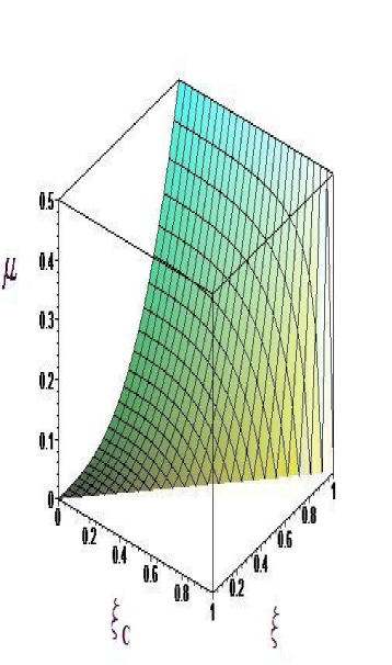
Figure 2:   The function $\mu(\xi;\xi_{C})\in[0,1/2]$ and the lines $\xi=const$ and $\xi_{C}=const$.          

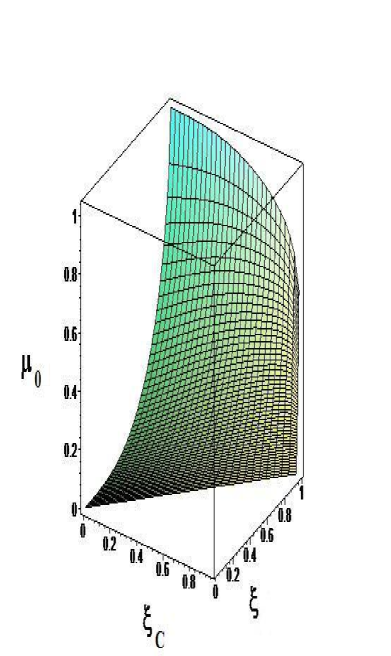
Figure 3:   The function $\mu_{0}(\xi;\xi_{C})$ and the lines $\xi=const$ and $\xi_{C}=const$.          

Instead of the local binding energy $\Delta m(\rho,\rho_{C}):=m_{0}-m$, which is not $\lambda$ -invariant, one can consider the ratio

$$\varrho(\rho,\rho_{C}):=m/m_{0}=\mu/\mu_{0}=\varrho(\xi,\xi_{C})\in(0,1).\hskip 14.22636pt$$ (III.12)

It measures in a $\lambda$ -invariant way the local mass defect of the star mater, i.e. the mass defect in the sphere with luminosity radius $\rho$ and center $C$.

Another important $\lambda$-invariant local (in the above sense) quantity is $f(\rho,\rho_{C})=\varrho(\rho,\rho_{C})^{2}-g_{tt}(\rho,\rho_{C})+1$. In the case at hand it has the form

$$f(\rho,\rho_{C})=\left({{m}\over{m_{0}}}\right)^{2}+{{2m}\over{\rho}}=\varrho^{2}+\varsigma^{2},$$ (III.13)

where $\varsigma^{2}\!=\!{{2m}\over{\rho}}\geq 0$ is the local compactness of the star. For incompressible stars $\varsigma^{2}={{\xi-\xi_{C}^{3}}\over{\xi(1-\xi_{C}^{3})}}$.

Using the results (A.5) and (A.6) of Appendix A, after some algebra one obtains the expressions:

$$\varrho(\xi,\xi_{C})^{-1}=3\,{{\sqrt{1-\xi_{C}^{3}}}\over{\xi^{3}-\xi_{C}^{3}}}\int\limits_{\xi_{C}}^{\xi}{{\xi^{3}d\xi}\over{\sqrt{-P_{4}(\xi,\xi_{C})}}}=$$

$${3}{{\sqrt{1-\xi_{C}^{3}}}\over{\xi^{3}-\xi_{C}^{3}}}\Big{(}J_{3|1}(\xi,\xi_{C})-J_{3|1}(\xi_{C},\xi_{C})\Big{)}\hskip 14.22636pt$$ (III.14)

and

$$\chi(\xi,\xi_{C})={3\over 2}\sqrt{1-\xi_{C}^{3}}\int\limits_{\xi_{C}}^{\xi}{{\xi^{4}d\xi}\over{\left(\sqrt{-P_{4}(\xi,\xi_{C})}\right)^{3}}}=$$

$${3\over 2}\sqrt{1-\xi_{C}^{3}}\Big{(}J_{4|3}(\xi,\xi_{C})-J_{4|3}(\xi_{C},\xi_{C})\Big{)}\hskip 28.45274pt$$ (III.15)

for the basic $\lambda$-invariant local quantities $\varrho$ and $\chi$.

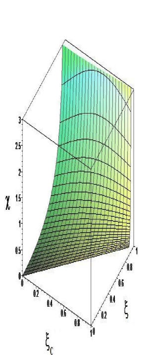
Figure 4:   The function $\chi(\xi;\xi_{C})$ and the lines $\xi=const$ and $\xi_{C}=const$. In contrast to $m_{0}(\xi;\xi_{C})$, the function $\chi(\xi;\xi_{C})$ is not bounded from above.          

As one sees, the technical problem of finding the general solution of ETOV system for incompressible matter in the most general case is reduced to the calculation of the elliptic integrals in Eqs. (III.10), (III.14) and (III.15). This calculation is described in the Appendix A.

IV Radius of Incompressible Stars

Now we are able to proof the existence of a finite coordinate radius $r_{*}<\infty$ of incompressible stars. It corresponds to some finite value of the luminosity variable $\xi_{*}<\infty$ and to some finite geometrical radius $R_{*}={\cal R}_{*}/\sqrt{8\pi\varepsilon\left(1-\xi_{C}^{3}\right)/3}<\infty$. (Here ${\cal R}_{*}$ is the dimensionless $\lambda$-invariant geometrical radius of the star.)

By definition, in $\lambda$-invariant terms the edge of the star is defined as a point $\xi_{*}$ at which

$$p(\xi_{*},\xi_{C})=0.$$ (IV.1)

Proposition 1: For all solutions of ETOV equations (II)-(II) with EOS (I.1) and arbitrary $\xi_{C}\geq 0$ there exist a unique solution $\xi_{*}\in\big{(}\xi_{C},\xi_{*}^{crit}(\xi_{C})\big{)}$ of the Eq. (IV.1). Here the value $\xi_{*}^{crit}(\xi_{C})\in(\xi_{C},1)$ corresponds to the nonphysical limiting solution with infinite value of the pressure at the stelar center: $p_{C}^{crit}=\infty$.

Proof:

1) Existence of unique solution of Eq. (IV.1):

From Eq. (III.6) and (III.15) one easily obtains in the limit $\xi\to 1-0$:

$$\sqrt{-g_{\rho\rho}(\xi,\xi_{C})}\,\propto\,\sqrt{{{1-\xi_{C}^{3}}\over{2+\xi_{C}^{3}}}{{1}\over{1-\xi}}}\to\infty,$$

$$\chi(\xi,\xi_{C})\,\propto\,3\,\sqrt{{{1-\xi_{C}^{3}}\over{\left(2+\xi_{C}^{3}\right)^{3}}}{{1}\over{1-\xi}}}\to\infty.$$ (IV.2)

Hence

$$\lim_{\xi\to 1-0}{{\sqrt{-g_{\rho\rho}(\xi,\xi_{C})}}\over{\chi(\xi,\xi_{C})}}={{2+\xi_{C}^{3}}\over{3}}\in(2/3,1).$$ (IV.3)

As a result

$$\lim_{\xi\to 1-0}w(\xi,\xi_{C})=-{{1-\xi_{C}^{3}}\over{3}}<0,$$ (IV.4)

i.e. the continuous, strictly monotonic function $w(\xi,\xi_{C})$ decreases on the interval $[\xi_{C},1]$ from some value $w_{C}=w(\xi_{C},\xi_{C})>0$ to the value $w(1,\xi_{C})=-{{1-\xi_{C}^{3}}\over{3}}<0$ (i.e., $w(\xi,\xi_{C})\!\searrow\![w_{C},\!-{(1\!-\!\xi_{C}^{3})/{3}}]$ for $\xi\in[\xi_{C},1)$). Then there exist a unique value $\xi_{*}\in(\xi_{C},1)$, such that $w(\xi_{*},\xi_{C})=0$. This value $\xi_{*}$ defines the radius of the star.

2) Limitations on the $\lambda$-invariant radius of star $\xi_{*}$:

The Eq. (II.10) permits us to rewrite the definition of the stelar radius (IV.1) in the following explicit form:

$$w_{C}\!=\!{{1}\over{\sqrt{-g_{\rho\rho}(\xi_{*},\xi_{C})}\!-\!\chi(\xi_{*},\xi_{C})}}\!-\!1\!=:w_{C}(\xi_{*},\xi_{C}).\hskip 19.91684pt$$ (IV.5)

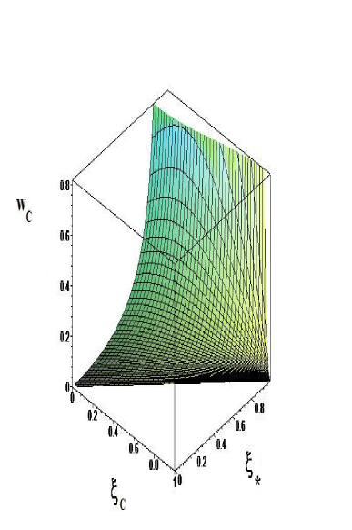
Figure 5:   The function $w_{C}(\xi_{*};\xi_{C})$ and the lines $\xi_{*}=const$ and $\xi_{C}=const$. Note that $w_{C}(\xi*;\xi_{C})=\infty$ on some special line $\xi_{*}=\xi_{*}^{crit}(\xi_{C})$ which will be studied in details in Subsection E of the present Section.          

It demonstrates the relation between the value $w_{C}$ at the center $C$ of the star and its radius $\xi_{*}$. This relation is the main difference between relativistic theory of stars and Newtonian one.

Using the following properties of the functions $\sqrt{-g_{\rho\rho}(\xi_{*},\xi_{C})}$ and $\chi(\xi_{*},\xi_{C})$

a) $-g_{\rho\rho}(\xi_{C},\xi_{C})=1$;

b) $\sqrt{-g_{\rho\rho}(\xi_{*},\xi_{C})}\nearrow[1,\infty)$, $\chi(\xi_{*},\xi_{C})\nearrow[0,\infty)$ – for $\xi\in[\xi_{C},1)$;

c) for $0<\xi-\xi_{C}\ll 1$: $\sqrt{-g_{\rho\rho}(\xi_{*},\xi_{C})}\!-\!\chi(\xi_{*},\xi_{C})>0$;

d) for $\xi\to 1$: $\sqrt{-g_{\rho\rho}(\xi_{*},\xi_{C})}/\chi(\xi_{*},\xi_{C})\propto(2+\xi_{C}^{3})/3\in(2/3,1)$; , one easily obtains that:

i) $w_{C}(\xi_{C},\xi_{C})=0$;

ii) $w_{C}(1,\xi_{C})=-1$;

ii) There exist a unique point $\xi_{*}^{crit}\in(\xi_{C},1)$, such that $\sqrt{-g_{\rho\rho}(\xi_{*}^{crit},\xi_{C})}=\chi(\xi_{*}^{crit},\xi_{C})\,\,\Rightarrow\,\,$ $w_{C}(\xi_{*}^{crit}-0,\xi_{C})=+\infty$ and $w_{C}(\xi_{*}^{crit}+0,\xi_{C})=-\infty$.

This means that there exist a limiting nonphysical solution – an incompressible star with a critical radius $\xi_{*}^{crit}\in(\xi_{C},1)$, which corresponds to an infinite pressure $p_{C}^{crit}=\infty$ at the center $C$. Hence, the $\lambda$-invariant radius of the incompressible stars is constraint in the interval $(\xi_{C},\xi_{*}^{crit})$. It is obvious that $\xi_{*}^{crit}$ is a function of $\xi_{C}$. At the end of this Section we shall obtain the equation for determining of the function $\xi_{*}^{crit}(\xi_{C})$ and study its solution in details.

This completes the proof of our Proposition.

The luminosity radius $\rho_{*}$ of the star can be find in the form $\rho_{*}={{\xi_{*}}\over{\xi_{C}}}\rho_{C}\geq\rho_{C}$ and is not bounded from above if $\varepsilon\to 0$, or/and for $\xi_{C}\to 1$.

Having in our disposal the $\lambda$-invariant radius $\xi_{*}$ of the star, we are able to introduce another basic $\lambda$-invariant characteristics:

i) The total Keplerian mass $\mu_{*}=\mu(\xi_{*},\xi_{C})\in(0,1/2)$ – for $0\leq\xi_{C}\leq\xi_{*}<1$, see Fig 2.

ii) The total proper mass $\mu_{0*}=\mu_{0}(\xi_{*},\xi_{C})>0$.

iii) The total mass defect ratio $\varrho_{*}=\varrho(\xi_{*},\xi_{C})>0$.

iv) The total compactness $\varsigma_{*}=\varsigma(\xi_{*},\xi_{C})\!=\!{{2m_{*}}/{\rho_{*}}}\!=\!{{\xi_{*}^{3}-\xi_{C}^{3}}\over{\xi_{*}(1-\xi_{C}^{3})}}\!\in\!(0,1)$, etc.

v) In addition we obtain the relations

$$\varphi_{*}=\varphi(\xi_{*},\xi_{C})=\ln\left(w_{C}+1\right)+\varphi_{C}$$ (IV.6)

and (see Appendix A):

$${\cal R}_{*}\!=\!{\cal R}_{*}(\xi_{*},\xi_{C})\!=\!\sqrt{1\!-\!\xi_{C}^{3}}\int_{\xi_{C}}^{\xi_{*}}\!\!{{\xi d\xi}\over{\sqrt{-P_{4}(\xi,\xi_{C})}}}=$$

$$\sqrt{1\!-\!\xi_{C}^{3}}\Big{(}J_{1|1}(\xi,\xi_{C})-J_{1|1}(\xi_{C},\xi_{C})\Big{)}.\hskip 14.22636pt$$ (IV.7)

It is easy to see that ${\cal R}_{*}(\xi_{*},\xi_{C})\to\infty$ when $\xi_{C}=0$ and $\xi_{*}\to 1-0$.

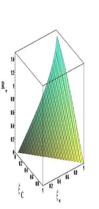
Figure 6:   A part of the function ${\cal R}_{*}(\xi_{*};\xi_{C})$ and the lines $\xi_{*}=const$ and $\xi_{C}=const$.          

As seen in Fig. 2 the function $\mu_{*}(\xi_{*},\xi_{C})$ has values in the interval $[0,1/2]$. At the same time we obtain a new

Proposition 2: In the specific limit: $\xi_{*}\to 1$, $\xi_{C}\to 1$, $0\leq\xi_{C}\leq\xi_{*}\leq 1$ we have

$$\lim_{\underset{\xi_{C}\leq\xi_{*}\leq 1}{\xi_{C}\to 1}}\mu_{*}(\xi_{*},\xi_{C})=:\mu_{*}(1\!-\!0,1\!-\!0)\in[0,1/2],\hskip 14.22636pt$$ (IV.8)

i.e., the limit $\mu_{*}(1\!-\!0,1\!-\!0)$ is bounded, but not definite and can have any value in the interval $[0,1/2]$.

The analytical proof becomes obvious from the representation $\mu_{*}(\xi_{*},\xi_{C})={1\over 2}{\over{1-\xi_{c}}}{{\xi_{*}^{2}+\xi_{*}\xi_{C}+\xi_{C}^{2}}\over{1+\xi_{C}+\xi_{C}^{2}}}$ and consideration of the limit $\xi_{C}\to 1$ of $\mu_{*}(\xi_{*},\xi_{C})$ on the curves $\xi_{*}=\xi_{C}+k(1-\xi_{C})$ with an arbitrary $k\in[0,1]$.

Note that for any $k\in[0,1]$ and $n>1,p>1$:

i) On the curves $\xi_{*}=\xi_{C}+k(1-\xi_{C}^{p})^{n}$ the limit (IV.8) has an universal value $0$.

ii) On the curves $\xi_{*}=1-k(1-\xi_{C}^{p})^{n}$ the limit (IV.8) has an universal value $1/2$.

Hence, the typical behavior of the limit (IV.8) is given by the last two cases: i) and ii). The case of linear dependence between $\xi_{*}$ and $\xi_{C}$ is an exceptional one.

The simple, but important property of the function $\mu_{*}(\xi_{*},\xi_{C})$, described in Proposition 2, will influence further results in the theory of incompressible relativistic stars, when the same limit of other quantities will emerge.

V The Basic $Rm$ Mapping for Incompressible Stars

The basic mapping

$$\{{\cal R}_{*},\mu_{*}\}\lx@xy@svg{\hbox{\raise 0.0pt\hbox{\kern 1.0pt\hbox{\ignorespaces\ignorespaces\ignorespaces\hbox{\vtop{\kern 0.0pt\offinterlineskip\halign{\entry@#!@&&\entry@@#!@\cr&\crcr}}}\ignorespaces{\hbox{\kern-1.0pt\raise 0.0pt\hbox{\hbox{\kern 0.0pt\raise 0.0pt\hbox{\hbox{\kern 1.0pt\raise 0.0pt\hbox{$\textstyle{{}\ignorespaces\ignorespaces\ignorespaces\ignorespaces}$}}}}}}}\ignorespaces\ignorespaces\ignorespaces\ignorespaces{}{\hbox{\lx@xy@droprule}}\ignorespaces\ignorespaces\ignorespaces{\hbox{\kern 4.24242pt\raise 5.39166pt\hbox{{}\hbox{\kern 0.0pt\raise 0.0pt\hbox{\hbox{\kern 3.0pt\hbox{\hbox{\kern 0.0pt\raise-2.39166pt\hbox{$\scriptstyle{Rm}$}}}\kern 3.0pt}}}}}}\ignorespaces{\hbox{\kern 25.0pt\raise 0.0pt\hbox{\hbox{\kern 0.0pt\raise 0.0pt\hbox{\lx@xy@tip{1}\lx@xy@tip{-1}}}}}}{\hbox{\lx@xy@droprule}}{\hbox{\lx@xy@droprule}}{\hbox{\kern 25.0pt\raise 0.0pt\hbox{\hbox{\kern 0.0pt\raise 0.0pt\hbox{\hbox{\kern 1.0pt\raise 0.0pt\hbox{$\textstyle{}$}}}}}}}\ignorespaces}}}}\ignorespaces\{\xi_{*}({\cal R}_{*},\mu_{*}),\xi_{C}({\cal R}_{*},\mu_{*})\}. \scriptstyle{Rm} \scriptstyle{Rm}$$ (V.3)

was defined in general case in F04NMGS . Here we study this mapping in the specific case of incompressible GRS in scale-invariant variables:

Substituting in the formula (IV.7) $\xi_{*}=\xi_{*}(\mu_{*},\xi_{C})$, or $\xi_{C}=\xi_{C}(\mu_{*},\xi_{*})$, obtained from the first of the relations (III.11) in the form

$$\xi_{*}(\mu_{*},\xi_{C})=\sqrt[3]{2\mu_{*}+(1-2\mu_{*})\xi_{C}^{3}},$$ (V.4a)

$$\xi_{C}(\mu_{*},\xi_{*})=\sqrt[3]{(\xi_{*}^{3}-2\mu_{*})/(1-2\mu_{*})},$$ (V.4b)

one obtains the functions ${\cal R}_{*}={\cal R}_{*}(\mu_{*},\xi_{C})$ and ${\cal R}_{*}={\cal R}_{*}(\mu_{*},\xi_{*})$ .

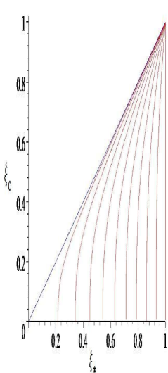
Figure 7:   The function $\xi_{C}=\xi_{C}(\mu_{*},\xi_{*})$ (V.4b) for different fixed values of parameter $\mu_{*}\in(0,1/2)$.          

The corresponding inverse functions $\xi_{*}=\xi_{*}(\mu_{*},{\cal R}_{*})$ and $\xi_{C}=\xi_{C}(\mu_{*},{\cal R}_{*})$ define the basic mapping $Rm$ (V.3) in $\lambda$-invariant terms. This mapping is illustrated in figures 8 and 9.

Figure 8:   The function $\xi_{*}(\mu_{*};{\cal R}_{*})\in[0,1]$. The behavior of this function in the limit $\mu_{*}\to 0,{\cal R}_{*}\to 0$ is similar to the one, described in Proposition 2 for the function $\mu_{*}(\xi_{*},\xi_{C})$.          

Figure 9:   The function $\xi_{C}(\mu_{*};{\cal R}_{*})\in[0,1]$. The behavior of this function in the limit $\mu_{*}\to 0,{\cal R}_{*}\to 0$ is similar to the one, described in Proposition 2 for the function $\mu_{*}(\xi_{*},\xi_{C})$.          

As a byproduct from Eq. (V.4b), $2\mu_{*}\leq 1$ and $\xi_{C}\geq 0$ we obtain a new inequality $\xi_{*}^{3}\geq 2\mu_{*}$. Then, since $0<\xi_{*}<1$, we have

$$0<{{2\mu_{*}}\over{\xi_{*}}}<{{2\mu_{*}}\over{\xi_{*}^{3}}}\leq 1.$$ (V.5)

For incompressible stars the relations, which determine the domain ${\mathbb{D}}^{(2)}_{\xi_{*}\xi_{C}}$ F04NMGS , acquire the following specific form (For the used notations see Appendix A.):

$$0\,\,\leq\,\,\xi_{C}\,\,\leq\,\,\xi_{*}\,\,<\,\,1,\hskip 128.0374pt$$ (V.6a)

$$-\xi_{*}(1+\xi_{*})\,\,\leq\,\,0\leq\,\,\xi_{C}^{3},\hskip 128.0374pt$$ (V.6b)

$$\sqrt{{{\xi_{*}}\over{(1-\xi_{*})(\xi_{C}^{3}+\xi_{*}^{2}+\xi_{*})}}}-{{1}\over{\sqrt{1-\xi_{C}^{3}}}}\,\,\,<\hskip 51.21504pt$$

$${3\over 2}\Big{(}J_{4|3}\left(\xi_{*},\xi_{C}\right))-J_{4|3}\left(\xi_{C},\xi_{C}\right)\Big{)}\!<\!\hskip 51.21504pt$$

$$\sqrt{{{\xi_{*}}\over{(1\!-\!\xi_{*})(\xi_{C}^{3}+\xi_{*}^{2}+\xi_{*})}}}\hskip 71.13188pt.$$ (V.6c)

As a result of the first of the relations (V.6) the condition (V.6b) is fulfilled.

Parts of the corresponding domains ${\mathbb{D}}^{(2)}_{\mu_{*},R_{*}}$ are shown in Figs. 10 and 11, where the condition (V.6c) is still not taken into account.

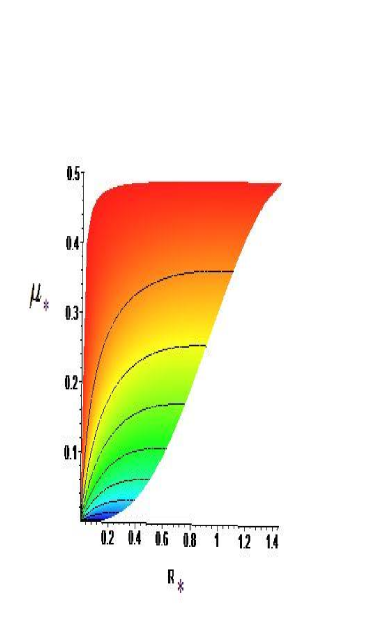
Figure 10:   The domain ${\mathbb{D}}^{(2)}_{\mu_{*},R_{*}}$ for the function $\xi_{C}(\mu_{*};{\cal R}_{*})$.          

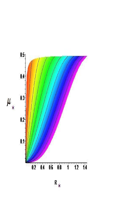
Figure 11:   The domain ${\mathbb{D}}^{(2)}_{\mu_{*},R_{*}}$ for the function $\xi_{C}(\mu_{*};{\cal R}_{*})$.          

VI The Critical Radius and Critical Mass of Incompressible Stars

The limiting case of Eq. (V.6c) yields the following equation for the critical value $\xi_{*}^{crit}=\xi_{*}^{crit}(\xi_{C})$ of the dimensionless luminosity variable:

$$J_{4|3}\left(\xi_{*}^{crit},\xi_{C}\right)\!-\!J_{4|3}\left(\xi_{C},\xi_{C}\right)\!=\!{{2\,\xi_{*}^{crit}}\over{3\sqrt{-P_{4}(\xi_{*}^{crit},\xi_{C})}}}.\hskip 22.76228pt$$ (VI.1)

It is obvious that this equation defines a new function $\xi_{*}^{crit}(\xi_{C})$, which describes the basic difference between GR and Newtonian incompressible stars. There are no any physical parameters in the Eq. (VI.1). Hence, the function $\xi_{*}^{crit}(\xi_{C})$ is an universal mathematical one.

In the degenerated Schwarzschild case when $\xi_{C}=0$ we have $-P_{4}(\xi,\xi_{C})=\xi^{2}(1-\xi^{2})$ and the integral in Eq. (VI.1) can be easily done. This gives (see Appendix A)

$${1\over{\sqrt{1-(\xi_{*}^{crit})^{2}}}}-1={2\over{3\sqrt{1-(\xi_{*}^{crit})^{2}}}}.$$

Hence,

$$\xi_{*}^{crit}(\xi_{C}=0)=\sqrt{8/9}\approx.942809.$$ (VI.2)

Thus we have obtained the exact value of the new function $\xi_{*}^{crit}(\xi_{C})$ at the point $\xi_{C}=0$. It is clear that $\xi_{*}^{crit}(\xi_{C}=1)=1$.

The shape of function $\xi_{*}^{crit}(\xi_{C})$ is shown in Fig. 12. Some of its basic values are given in Appendix B.

Figure 12:   The function $\xi_{*}^{crit}(\xi_{C})$ as a border of the physical domain of the variable $\xi_{*}\in\big{(}\xi_{C},\xi_{*}^{crit}(\xi_{C})\big{)}$.          

As seen, the values of the function $\xi_{*}^{crit}(\xi_{C})$ are in the interval $[\sqrt{8/9},1]$. Hence, for a given value of $\lambda$-invariant luminosity variable $\xi_{C}>0$, the value of $\xi_{*}$ varies in the interval $[\xi_{C},\xi_{*}^{crit}(\xi_{C})]$, with upper limit $\xi_{*}^{crit}(\xi_{C})>\sqrt{8/9}$.

This changes radically our understanding of the relativistic theory of stars, because now in the domain $0\leq\xi_{C}\leq\xi_{*}\leq 1$:

$${{2m_{*}}\over{\rho_{*}}}=\varsigma_{*}={{\xi_{*}^{3}-\xi_{C}^{3}}\over{\xi_{*}(1-\xi_{C}^{3})}}\leq\xi_{*}^{2}<\Big{(}\xi_{*}^{crit}(\xi_{C})\Big{)}^{2}.\hskip 11.38092pt$$ (VI.3)

As a result of the last inequality one obtains the familiar relativistic restriction for the Schwarzschild degenerate case:

$$\Big{(}2m_{*}/\rho_{*}\Big{)}_{\xi_{C}=0}=\varsigma_{*}{}_{\big{|}_{\xi_{C}=0}}=\xi_{*}^{2}<8/9.$$

This constraint yields the following restrictions on the luminosity variable and Keplerian mass of Schwarzschild incompressible stars:

$$\rho_{*}{}_{\big{|}_{\xi_{C}=0}}<{1\over{\sqrt{3\pi\varepsilon}}},\,\,\,\,m_{*}{}_{\big{|}_{\xi_{C}=0}}<{4\over 9}{1\over{\sqrt{3\pi\varepsilon}}}.$$ (VI.4)

Hence, in the relativistic model with $\rho_{C}=0$ we are not able to describe stars with fixed density $\varepsilon=const$ and with arbitrary large mass $m_{*}$.

In contrast, in our general geometrical model of incompressible relativistic stars with arbitrary fixed value of luminosity variable $\xi_{C}\in[0,1]$ we have the restrictions:

$$\rho_{*}<\rho_{*}^{crit}\!:=\!{1\over{\sqrt{8\pi\varepsilon/3}}}{{\xi_{*}^{crit}(\xi_{C})}\over{\sqrt{1\!-\!\xi_{C}^{3}}}}\to\infty:\,\,\,\hbox{for}\,\,\xi_{C}\!\to\!1\!-\!0,$$

$$m_{*}<\!m_{*}^{crit}\!:=\!{1\over 2}{1\over{\sqrt{8\pi\varepsilon/3}}}{{\left(\xi_{*}^{crit}(\xi_{C})\right)^{3}\!-\!\xi_{C}^{3}}\over{\left(\sqrt{1\!-\!\xi_{C}^{3}}\right)^{3}}}\to\infty:\hskip 19.91684pt$$ (VI.5)

$$\,\,\,\hbox{for}\,\,\xi_{C}\to 1-0.$$

These upper limits $\rho_{*}^{crit}(\xi_{C})$ and $m_{*}^{crit}(\xi_{C})$ are exact, i.e., the corresponding quantities $\rho_{*}$ and $m_{*}$ can become arbitrary close to them for a given value of $\xi_{C}$.

The calculation of the limit of $\rho_{*}^{crit}(\xi_{C})$ is obvious from $\xi_{*}^{crit}(\xi_{C}=1-0)=1$, see Fig. 12. The analytical proof of the above limit for $m_{*}^{crit}(\xi_{C})$ when $\xi_{C}\to 1-0$ follows immediately from our Proposition 3 (see Section IV, C) and Eq.(III.10). The behavior of the critical mass $m_{*}^{crit}(\xi_{C})$ as a function of the central value $\xi_{C}$ of luminosity variable is shown in Fig. 13 for density $32\pi\varepsilon/3=1$ .

Figure 13:   The critical mass of the star $m_{*}^{crit}(\xi_{C})$ as a border of the physical domain of the variable $m_{*}\in\big{(}0,m_{*}^{crit}(\xi_{C})\big{)}$.          

Thus we have arrived at the following

Proposition 3: For any fixed density $\varepsilon=const$ in our essentially non-Euclidean general model of relativistic stars there exist incompressible stars with arbitrary large mass $m_{*}$.

Obviously, stars with arbitrary large mass $m_{*}$ exist only for large enough values of luminosity variable $\xi_{C}$.

From Eq. (IV.7) one obtains the following critical value for the geometrical radius of our relativistic incompressible stars:

$$R_{*}^{crit}(\xi_{C})\!=\!{J_{1|1}\big{(}\xi_{*}^{crit}(\xi_{C}),\xi_{C}\big{)}-J_{1|1}\big{(}\xi_{C},\xi_{C}\big{)}\over{\sqrt{8\pi\varepsilon/3}}}.\hskip 14.22636pt$$ (VI.6)

The behavior of the critical geometrical radius $R_{*}^{crit}(\xi_{C})$ as a function of the central value $\xi_{C}$ of luminosity variable is shown in Fig. 14 for density $32\pi\varepsilon/3=1$.

Figure 14:   The critical geometrical radius of the star $R_{*}^{crit}(\xi_{C})$ as a border of the physical domain of the geometrical stelar radius $R_{*}\in\big{(}R_{*}^{crit}(\xi_{C}),\infty\big{)}$.          

Thus, we have proved the existence of new amazing regular relativistic objects with constant matter density: They can have an arbitrary large mass $m_{*}$. As a result of strong gravity, their geometrical radius $R_{*}$ and luminosity $L_{*}\sim 1/\rho_{*}^{2}$ are arbitrary small, when the mass $m_{*}$ is large enough. At the same time in presence of such objects the geometry of the space-time is regular everywhere. Horizons of any type do not exist.

It seems reasonable to refer to objects as to heavy black dwarfs. As seen in Fig. 13, the existence of HBD is impossible under widely accepted extra condition $\rho_{c}=0$.

The critical proper mass $m_{0*}^{crit}(\xi_{C})$ is bigger then $m_{*}^{crit}(\xi_{C})$. Hence, it goes to infinity in the limit $\xi_{C}\to\infty$ together with $m_{*}^{crit}(\xi_{C})$.

More interesting characteristic is the $\lambda$-invariant critical mass defect ratio $\varrho_{*}^{crit}(\xi_{C})$, obtained from Eq. (III.14) in the form:

$$\varrho_{*}^{crit}(\xi_{C})=\hskip 145.10922pt$$ (VI.7)

$${{\big{(}\xi_{*}^{crit}(\xi_{C})\big{)}^{3}-\xi_{C}^{3}}\over{3\Big{(}J_{3|1}\big{(}\xi_{*}^{crit}(\xi_{C}),\xi_{C}\big{)}\!-\!J_{3|1}\big{(}\xi_{C},\xi_{C}\big{)}\Big{)}\sqrt{1\!-\!\xi_{C}^{3}}}}.$$

This function is represented in Fig. 15.

Figure 15:   The critical mass ratio $\varrho_{*}^{crit}(\xi_{C})$ as a border of the physical domain of the variable $\varrho_{*}\in\big{(}\varrho_{*}^{crit}(\xi_{C}),1\big{)}$. (In the Fig 15 the symbol $V\!\rho$ stands for $\varrho$.)          

As seen, the critical value of the mass ratio $\varrho_{*}^{crit}(\xi_{C})$ decreases monotonically from

$$\varrho_{*}^{crit}(0)={16\over 9}\Bigg{(}1-3\sqrt{9\over 8}\arcsin\left(\sqrt{8\over 9}\right)\Bigg{)}^{-1}\approx.609477$$

to $1/2$ when the variable $\xi_{C}$ increases from $0$ to $1$.

Hence, in the case of incompressible mater the extremely strong gravitational field, which arise in the limit $R_{*}\to 0$, $m_{*}\to\infty$ is able to extract no more then one halve of the initial bare mass $m_{0*}$ of the stelar matter, although the relative part of gravitational energy increases in this limit, together with the mass defect. It can be shown that this limitation is EOS-dependent.

One can understand the above behavior of the critical mass ratio $\varrho_{*}^{crit}(\xi_{C})$ analyzing the form of the functions $\mu_{*}^{crit}(\xi_{C})$ – Fig. 16 and $\mu_{0*}^{crit}(\xi_{C})$ – Fig. 17:

Figure 16:   The critical function $\mu_{*}^{crit}(\xi_{C})$ as a boundary of the physical domain of the variable $\mu_{*}\in\big{(}0,\mu_{*}^{crit}(\xi_{C})\big{)}$. As seen, on the specific curve $\xi_{*}=\xi_{*}^{crit}(\xi_{C})$ the function $\mu_{*}^{crit}(\xi_{C})$ goes to $1/2$, when $\xi_{C}\to 1$. (Compare this specific result with Proposition 2 and with comments after it.)          

Figure 17:   The critical function $\mu_{0*}^{crit}(\xi_{C})$ as a boundary of the physical domain of the variable $\mu_{0*}\in\big{(}0,\mu_{0*}^{crit}(\xi_{C})\big{)}$.          

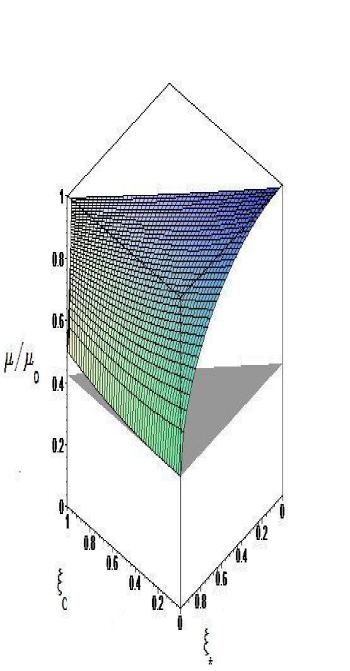
Figure 18:   The function $\varrho(\xi_{*},\xi_{C})=\mu(\xi_{*},\xi_{C})/\mu_{0}(\xi_{*},\xi_{C})\geq 4/3\pi$ for incompressible star. The shadowed triangle is a part of the horizontal plane $4/3\pi\approx.424413$.          

A more deep understanding of the mass defect one can obtain looking on 3D surface of the function, $\varrho(\xi_{*},\xi_{C})=\mu(\xi_{*},\xi_{C})/\mu_{0}(\xi_{*},\xi_{C})\geq 4/3\pi$, shown in Fig. 18. The last limit from below of the mass ratio $\varrho(\xi_{*},\xi_{C})$ originates from EOS for incompressible stars Eq. (I.1) and will be different for relativistic stars with other EOS. It reflects the form of the right border of the 3D surface:

$$\varrho_{*}(\xi_{*},0)={2\over 3}{{\xi_{*}^{3}}\over{\arcsin\xi_{*}-\xi_{*}\sqrt{1-\xi_{*}^{2}}}},$$ (VI.8)

calculated for the Schwarzschild degenerate case of incompressible stars. An analogous simple expression can be drown for $\varrho\left(\xi_{*},\sqrt[3]{1/4}\right)$, using results, given in Appendix A.

The real limit from below on $\varrho(\xi_{*},\xi_{C})$ in the problem at hands is $1/2$. It reflects the existence of the curve $\xi_{*}^{crit}(\xi_{C})$, which is not shown in Fig.18.

VII Mass-Radii Relations for White Dwarfs and the New Geometrical Models of GRS

Our previous consideration F04NMGS showed that there exist two different approaches to the GRS with stiff mass-radii functional dependence:

1) The standard one, based on the extra condition $\rho(0)\equiv\rho_{C}=0$, and

2) A new one, with extra condition: $\digamma$– fixed. It arises naturally in basic regular radial gauge F04NMGS . Here $\digamma\in(-\infty,\infty)$ is the stelar crust parameter. It defines the jump of the derivative of luminosity variable $\rho(r)$ as a function of the radial one, $r$ : $\rho^{\prime}(r_{*}-0)=e^{-\digamma}\rho^{\prime}(r_{*}+0)$, at the edge of the star $r_{*}$.

At the same time one can consider a geometrical models of GRS without any additional condition of that type. In this most general case stiff mass-radii relations, based only on GR considerations, i.e. independent on EOS, do not exist F04NMGS . In this case $m_{*}$ and $R_{*}$ are free parameters, constrained in some 2D domain, the precise form of which depends on the EOS.

The physical domain of variables $m_{*}$ and $R_{*}$ for incompressible GRS is shown in Fig. 19.

Figure 19:   The function $R_{*}^{crit}(m_{*}^{crit})$ as a boundary of physical domain for incompressible star with energy density ${{32}\over 3}\pi\varepsilon=1$.          

It is obvious that this physical domain is very similar to the one, recently observed for real white dwarfs, see Fig. 2 in the article by J. Madej, M. Naleźyty and L. G. Althaus in WD . This demonstrates how we are able to reproduce the real observational data in a qualitatively right way, using the simplest new geometrical model of incompressible GRS.

The most important consequence of our analysis of the observational data is the conclusion that actually we do not observe stiff mass-radii relations in Nature. Instead, these data demonstrate a clear indication that $m_{*}$ and $R_{*}$ are filling a 2D domain with a sharp boundary of the type, similar to the one, shown in our Fig. 19. This corresponds to our general models of GRS without any extra conditions F04NMGS . Therefore we will skip the consideration of such relations in the present article, although they may be of some interest, too.

For a more precise qualitative treatment of the observational data one need to obtain new geometrical models of the GRS with realistic EOS. This may give a basis for explanation of the mass distributions of special type of stars, like white dwarfs, or neutron stars, independently of theory of gravity. We will present the corresponding results elsewhere.

VIII Concluding Remarks

In conclusion several remarks have to be made:

1. In the present article we have recovered an interesting new GR phenomena, studying the most general solutions of ETOV equations for incompressible matter. We were able to find proper physical meaning of all solutions of these equations, overcoming the requirement for regularity of solutions at the zero value of the luminosity variable $\rho$. As we have seen, this way we obtain a two parameters family of solutions.

2. We wish to comment once more the most important result of present article: the proof of the existence of new GR objects – heavy black dwarfs (HBD).

From physical point of view this becomes possible, because the fulfilment of the condition $\rho\geq\rho_{C}>\rho_{G}$ F04NMGS , where $\rho_{G}=2m_{*}$ is the Schwarzschild radius, is equivalent to the introduction of non-permeable potential wall in the space of the luminosity variable $\rho$. Because of the Gauss theorem, this introduces in the energy balance of the body an effective ”potential energy” with an infinite jump.

Then, following the original Landau energetic consideration of the problem Landau , we conclude that the presence of any additional energy terms, due to EOS, can not destroy the existence of static equilibrium of the body, at least in the case of non-ultra-relativistic matter. This ”$\rho$-space picture” explains in a more usual language the consequences of the new boundary conditions at the real center of the star, under which we are solving Einstein equations. See for details F04NMGS .

In terms of the proper radial variable $r$ no wall exist at all. Thus we see once more, that one is to give up the idea to consider the luminosity variable $\rho$ as a measure of distances. It is responsible only for determination of geometrical area and luminosity of physical objects.

3. The results of the present article raise many new questions and problems.

For example, we obtain a new real alternative to the black holes (BH) for explanation of nature of the massive compact dark objects, observed in astrophysics. Hence, we need a new criteria to distinguish BH and HBD.

An obvious problem is the possible relation of HBD with the observed could dark matter in the universe, as well as the relation of HBD with gravitational collapse of usual bodies. It is clear, that the present series of articles calls for a novel consideration of the collapse, too.

For a comparison with observational data, we obviously need consideration of new geometrical models of GRS with more realistic EOS for stelar matter.

We intend to address all these questions in the forthcoming articles in this series.

Acknowledgments

The author is grateful to the JINR, Dubna for financial support of the present article and for the hospitality and good working conditions during his two three-months visits in 2003 and in 2004, when the most of the work has been done.

The author is deeply indebted to Prof. T. L. Boyadjiev for friendly support and many useful discussions on mathematical problems, related to the stelar boundary problem, to Prof. S. Bonazzola, for discussions, and especially, for encouraging general information about the existence of results in direction of overcoming of the standard relativistic restriction on the stelar masses. Similar results can be found in the articles Bell , too. The author wishes to thank Prof. Ll. Bell for attracting his attention to these articles.

The author is grateful, too, to E.-M. Pauli and to M. Miller for discussions on white dwarfs’ physics and for information about available data. Special tanks to E.-M. Pauli for sending the file of her PhD thesis.

Appendix A Calculation of the Elliptic Integrals

Using standard incomplete elliptic integrals of first, second and third kind ($F$, $E$ and $\Pi$) elliptic , we can write down the integrals

$$J_{n|m}(\xi,\xi_{C}):=\int\!d\xi\,{{\xi^{n}}\Big{/}\left({\sqrt{-P_{4}(\xi,\xi_{C})}}\right)^{m}},$$ (A.1)

which are needed for the relativistic incompressible star problem, in the following form:

I. $n=0$, $m=1$:

$$J_{0|1}(\xi,\xi_{C})=g\,{1\over i}F(iz,k),$$ (A.2)

In the generate cases one obtains:

a)   $J_{0|1}(\xi,0)={1\over 2}\ln\left({{1-\sqrt{1-\xi^{2}}}\over{1+\sqrt{1-\xi^{2}}}}\right);$

b)  $J_{0|1}(\xi,\sqrt[3]{1/4})={2\over{\sqrt{3}}}\arctan\left({{\sqrt{3}(-1+4\xi)}\over{6\sqrt{\xi(1-\xi)}}}\right).$

II. $n=1$, $m=1$:

$$J_{1|1}(\xi,\xi_{C})=g\,{1\over i}F(iz,k)+g\,{1\over i}\Pi(iz,\alpha^{2},k),$$ (A.3)

In the generate cases one obtains:

a)   $J_{1|1}(\xi,0)=\arcsin(\xi);$

b)  $J_{1|1}(\xi,\sqrt[3]{1/4})\!=\!{{1}\over{3}}\sqrt{3}\arctan\left(\!{{\sqrt{3}(1-4\xi)}\over{6\sqrt{\xi(1-\xi)}}}\!\right)\!-\!\arcsin(1\!-\!2\xi)$.

II. $n=2$, $m=1$:

$$J_{2|1}(\xi,\xi_{C})={{1-3\sigma}\over 4}g\,{1\over i}F(iz,k)+$$

$${2\over g}\,{1\over i}E(iz,k)-{{\sqrt{-P_{4}(\xi,\xi_{C})}}\over{1-\xi}},$$ (A.4)

In the generate cases one obtains:

a)   $J_{2|1}(\xi,0)=1-\sqrt{1-\xi^{2}};$

b)  $J_{2|1}(\xi,\sqrt[3]{1/4})=-\sqrt{\xi(1-\xi)}-{{\sqrt{3}}\over{6}}\arctan\left(\!{{\sqrt{3}(1-4\xi)}\over{6\sqrt{\xi(1-\xi)}}}\!\right).$

II. $n=3$, $m=1$:

$$J_{3|1}(\xi,\xi_{C})={{2-\xi_{C}^{3}}\over 4}\,g\,{1\over i}F(iz,k)-$$

$${{1-\xi_{C}^{3}}\over 2}\,g\,{1\over i}\Pi(iz,\alpha^{2},k)-{1\over 2}\sqrt{-P_{4}(\xi,\xi_{C})},$$ (A.5)

In the generate cases one obtains:

a)   $J_{3|1}(\xi,0)={1\over 2}\arcsin(\xi)-{1\over 2}\xi\sqrt{1-\xi^{2}};$

b)  $J_{3|1}(\xi,\sqrt[3]{1/4})={{\sqrt{3}}\over{12}}\arctan\left(\!{{\sqrt{3}(1-4\xi)}\over{6\sqrt{\xi(1-\xi)}}}\!\right)-\\ \hbox{\hskip 42.67912pt}{3\over 8}\arcsin(1-2*\xi)-{1\over 4}(1+2\xi)\sqrt{\xi(1-\xi)}.$

II. $n=4$, $m=3$:

$$J_{4|3}(\xi,\xi_{C})\!=\!{{(1+\sigma)(\sigma^{2}-6\sigma-3)}\over{\sigma(3+\sigma)(9-\sigma^{2})}}\,g\,{1\over i}F(iz,k)+$$

$$\left({{2(3+\sigma^{2})}\over{\sigma(9-\sigma^{2})}}\right)^{2}{2\over g}\,{1\over i}E(iz,k)-$$

$${{\xi\left(2(3+\sigma^{2})\xi+(1-\sigma^{2})(3-\sigma^{2})\right)}\over{\sigma^{2}(9-\sigma^{2})\sqrt{-P_{4}(\xi,\xi_{C})}}}\,.$$ (A.6)

In the generate cases one obtains:

a)   $J_{4|3}(\xi,0)=1/\sqrt{1-\xi^{2}}-1;$

b)  $J_{4|3}(\xi,\sqrt[3]{1/4})={5\over{27}}\sqrt{3}\arctan{\left({{\sqrt{3}(1-4\xi)}\over{6\sqrt{\xi(1-\xi)}}}\right)}+\\ \hbox{\hskip 85.35826pt}{1\over 18}{{4\xi^{2}+15\xi+5}\over{(\xi-1/2})^{2}}\sqrt{{{\xi}\over{1-\xi}}}-{{5\pi\sqrt{3}}\over{54}}$.

Here $\sigma:=\sqrt{1-4\xi_{C}^{3}}$,    $z:=\alpha^{-1}\sqrt{\xi/(1-\xi)}$,

$$g:={4\over{\sqrt{(1+\sigma)(3-\sigma)}}},$$

$$k:=\sqrt{{{1-\sigma}\over{1+\sigma}}\,{{3+\sigma}\over{3-\sigma}}},$$

$$\alpha:=\sqrt{{{1-\sigma}\over{3-\sigma}}},\,\,\,\hbox{and}$$ (A.7)

$${1\over i}F(iz,k):=\int_{0}^{z}{{dx}\over{\sqrt{(1+x^{2})(1+k^{2}x^{2})}}},\hskip 42.67912pt$$ (A.8a)

$${1\over i}E(iz,k):=\int_{0}^{z}\sqrt{{{1+k^{2}x^{2}}\over{1+x^{2}}}}dx,\hskip 71.13188pt$$ (A.8b)

$${1\over i}\Pi(iz,\alpha^{2},k):=\!\int_{0}^{z}\!\!{{dx}\over{\!(1\!+\!\alpha^{2}x^{2})\!\sqrt{\!(1\!+\!x^{2})(1\!+\!k^{2}x^{2})}}\!}\hskip 8.5359pt$$ (A.8c)

define for any values $0\!\leq\!\xi_{C}\!\leq\!\xi\!<1$ three basic elliptic integrals in most convenient for us uniform representation.

Note that for $\xi_{C}\in\big{[}0,\sqrt[3]{1/4}\,\big{]}$ the parameters (A.7) have real values: $k\in\big{[}0,1\big{]}$, $g\in\big{[}2,4/\sqrt{3}\big{]}$, $\alpha\in\big{[}0,1/\sqrt{3}\big{]}$.

For $\xi_{C}\in\big{(}\sqrt[3]{1/4},1\big{)}$ these parameters are complex numbers. Nevertheless, for $0\leq\xi_{C}\leq\xi<1$ the integrals (A.2)-(A.6) have real values in this case, too.

Of course one can use more complicated representations of the standard elliptic integrals elliptic , such that the integrals $J_{n|m}(\xi,\xi_{C})$ will have transparently real values for $\xi_{C}\in\big{(}\sqrt[3]{1/4},1\big{)}$:

Taking into account that in this case $k=\exp(i\psi)$, $\psi\in\Re$, we can perform the transformation of the modulus $k\to\tilde{k}={1\over 2}\left(\sqrt{k}+1/\sqrt{k}\right)=\cos(\psi/2)\in[0,1]$ in all elliptic integrals. For example, $F(z,k)=F(\tilde{z},\tilde{k})/2\sqrt{k}$, where $\tilde{z}^{-1}={1\over 2}\left(z\sqrt{k}+1/z\sqrt{k}\right)$. Unfortunately, such representations for $E(z,k)$ and $\Pi(z,\alpha,k)$ are quite complicated. We will not give them here. They can be obtained composing several transformations of $k$, described in elliptic .

Appendix B Table of the values of function $\xi_{*}^{crit}(\xi_{C})$

Table 1: The values of function $\xi_{*}^{crit}(\xi_{C})$

$\xi_{C}$	$\Big{|}$	0.00	0.05	0.10	0.15	0.20	0.25	0.30
$\xi_{*}^{crit}$	$\Big{|}$	.9428	.9430	.9436	.9448	.9467	.9493	.9525
$\xi_{C}$	$\Big{|}$	0.35	0.40	0.45	0.50	0.55	0.60	0.65
$\xi_{*}^{crit}$	$\Big{|}$	.9564	.9608	.9 656	.9706	.9756	.9806	.9852
$\xi_{C}$	$\Big{|}$	0.70	0.75	0.80	0.85	0.90	0.95	1.00
$\xi_{*}^{crit}$	$\Big{|}$	.9894	.9930	.9959	.9980	.9993	.9999	1.00

References

(1) P. P. Fiziev, Novel Geometrical Models of Relativistic Stars.
The General Scheme, astro-ph/0409456
(2) L. D. Landau, E. M. Lifshitz, The Classical Theory of
Fields, 2d ed.; Reading, Mass: Addison-Wesley, 1962;
V. A. Fock, The Theory of Space, Time and Gravitation,
Pergamon, Oxford, 1964.
B. K. Harrison, K. S. Thorne, M. Wakano,
J. A. Wheeler, Gravitational Theory and Gravitational
Collapse, University of Chikago Press, 1965.
R. C. Tolman, Reativity, Thermodynamics and
Cosmology, Claderon Press, Oxford, 1969.
S. Weinberg, Gravitation and Cosmology, Wiley,
N.Y., 1972;
C. Misner, K. S. Thorne, J. A. Wheeler, Gravity,
W. H. Freemand & Co., 1973.
R. Adler, M. Bazin, M. Schiffer, Introduction to General
Relativity, McGraw-Hill Book Comp., 1965.
D. Kramer, H. Stephani, M. Maccallum,
E. Herlt, Ed. E. Schmutzer, Exact Solutions of the Einstein
Equations, Deutscher Verlag der
Wissenschaften, Berlin, 1980.
S. L. Shapiro, S. A. Teukolsky, Black Holes, White Dwarfs and Neutron
Stars, Jhon Wiley & Sons, 1985.
H. Stephani, General Relativity. An introduction to the theory of the gravitational field, 2nd
edition, Cambridge University Press, 1990.
G. S. Saakjan, The Physics of Neutron
Stars, 2nd eddition, Ereven University Press, 1988.
H. Stephani, D. Kramer, M. Maccallum,
E. Herlt, Exact Solutions of Einstein’s
Field Equations, 2nd eddition, Cambridge University
Press, 2003.
(3) Schwarzschild K., Sitz. Preuss. Acad.
Wiss., 424 (1916).
(4) S. Chandrasekhar, Ap. J. 74, 81 (1931); MNRAS, 95, 207 (1935).
L. Landau, Physik Zeits. Sowiet Union 1, 285 (1932).
S. Chandrasekhar, MNRAS 93, 390 (1933).
T. Hamada, E. E. Salpeter, ApJ 134, 683
(1961).
M. A. Wood, in Proc. 9th European Workshop on
White Dwarfs, ed. D. Koester, K. Werner,
Springer, 41, 1990.
(5) J. L. Grenstein, J. B. Oke, H. L. Shipman, ApJ, 169, 563 (1971).
H. L. Shipman, ApJ, 177, 723 (1972).
H. L. Shipman, ApJ, 213, 138 (1977).
H. L. Shipman, ApJ, 228, 240 (1979).
H. L. Shipman, C. A. Saas, ApJ., 235, 177 (1980).
S. Vennes, J. R. Thorstensen, P. Thejll, H. L. Shipman,
ApJ, 372, L37 (1991).
J. L. Provencal, H. L. Shipman, E. Hg, P. Thejll,
ApJ, 494, 759 (1998).
J. A. Panel, L. G. Althaus, O. G. Benvenuto, Astron.
Astrophys., 353, 970 (2000).
E.-M. Pauli, PhD Thesis, Der Friedrich-Alexander
Universität, Erlangen-Nürnberg, 2004.
J. Madej, M. Naleźyty, L. G. Althaus, Mass Distribution of DA White Dwarfs in
the First Data Release of Sloan Digital Sku Survey,
astro-ph/0404344.
(6) H. Bondi,Proc, Roy. Soc. (London), A 281, 39 (1964).
H. Bondi, Mon. Not. Roy. Astr. Soc. 107, 410 (1947).
H. A. Buchdahl, Phys. Rev. 116, 1027 (1959).
J. B. Hartle, Phys. Rep. 46, 202 (1978).
G. F. R. Ellis, R. Maartens, S. D. Neil,
M. N. R. A. S.184, 439 (1978).
C. B. Collins, J. Math. Phys. 26, 2268 (1985).
(7) H. Bateman, A. Erdélyi, Hgher Transcedental
Functions, Vol. 3, Mc Graw-Hill, 1955.
M. Abramowitz, I. A. Stegun, Handbook of Mathematical
Functions, Dover, 1964.
W. Mqgnus, F. Oberhettinger, R. P. Soni, em Formulas and Theorems for
the Special Functions of Mathematical Physics,
Springer, 1966.
P. F. Byrd, M. D. Friedman, Handbook of Elliptic Integrals for
Engineers and Scientists, Sec. Ed., Springer,
1971.
(8) J. M. Aguirregabiria, Ll. Bel, J. Martin, A. Molina, E. Ruiz
gr-qc/0104019, Gen. Rel. and Grav. 33 1809 (2001);
J. M. Aguirregabiria, Ll. Bel, gr-qc/0105043,
Gen. Rel. and Grav. 33, 2049 (2001) ;
Ll. Bel, gr-qc/0210057.
(9) L. Landau, Physik Zeits. Sowiet Union 1, 285 (1932).
L. D. Landau, E. M. Lifshitz, Course on Theoretical Physics,
Statistical Physics, Part 1, Oxford: Pergamon Press, 1980.