On the Period Distribution of Close-In Extrasolar Giant Planets

Abstract

Transit (TR) surveys for extrasolar planets have recently uncovered a population of “very hot Jupiters,” planets with orbital periods of $P\leq 3~{}\rm d$. At first sight this may seem surprising, given that radial velocity (RV) surveys have found a dearth of such planets, despite the fact that their sensitivity increases with decreasing $P$. We examine the confrontation between RV and TR survey results, paying particular attention to selection biases that favor short-period planets in TR surveys. We demonstrate that, when such biases and small-number statistics are properly taken into account, the period distribution of planets found by RV and TR surveys are consistent at better than the $1\sigma$ level. This consistency holds for a large range of reasonable assumptions. In other words, there are not enough planets detected to robustly conclude that the RV and TR short-period planet results are inconsistent. Assuming a logarithmic distribution of periods, we find that the relative frequency of very hot Jupiters (VHJ: $P=1-3~{}\rm d$) to hot Jupiters (HJ: $P=3-9~{}\rm d$) is $\sim 10-20\%$. Given an absolute frequency of HJ of $\sim 1\%$, this implies that approximately one star in $\sim 500-1000$ has a VHJ. We also note that VHJ and HJ appear to be distinct in terms of their upper mass limit. We discuss the implications of our results for planetary migration theories, as well as present and future TR and RV surveys.

1. Introduction

Radial velocity (RV) surveys have yielded a wealth of information about the ensemble physical properties of extrasolar planets. This information, in turn, provides clues to the nature of planetary formation and evolution. The period distribution of planets is particularly interesting in this regard. The very existence of massive planets at periods of $P\lesssim 10~{}\rm d$ was initially a surprise. Such planets are found around $\sim 1\%$ of main-sequence FGK stars (Marcy et al., 2003), and have likely acquired their remarkable real estate via migration through their natal disks after they accumulated the majority of their mass. Figure 1 shows the period distribution of short-period extrasolar planets detected in RV surveys. We have included companions with $M_{p}\sin i>0.2~{}M_{J}$ and $P\lesssim 10~{}\rm d$, corresponding to velocity semi-amplitudes of $K\gtrsim 20~{}{\rm m~{}s^{-1}}$ for solar-mass primaries and circular orbits; we expect RV surveys in this region of parameter space to be essentially complete. Significantly, roughly half of the 19 planets in this sample with $P\lesssim 10~{}\rm d$ have periods in the range $P\simeq 3-3.5~{}\rm d$. There is a sharp cutoff below this pile-up of planets, and there is only one planet with $P<3~{}\rm d$, the companion to HD73256 with $P\simeq 2.5~{}\rm d$. This planet is $\sim 3$ standard deviations away from the clump of planets in the range of $P=3-3.5~{}\rm d$, and so may be distinct in terms of its genealogy. Because RV surveys are likely to be substantially incomplete for planets with mass $M_{p}\sin i\lesssim 0.1~{}M_{J}$, we do not consider the recent RV discoveries of Neptune-mass planets with periods of $P=2.644~{}\rm d$ (GJ 436b; Butler et al. 2004), $P=2.808~{}\rm d$ (55 Cnc e; McArthur et al. 2004), and $P=9.55~{}\rm d$ ($\mu$ Arae c; Santos et al. 2004).

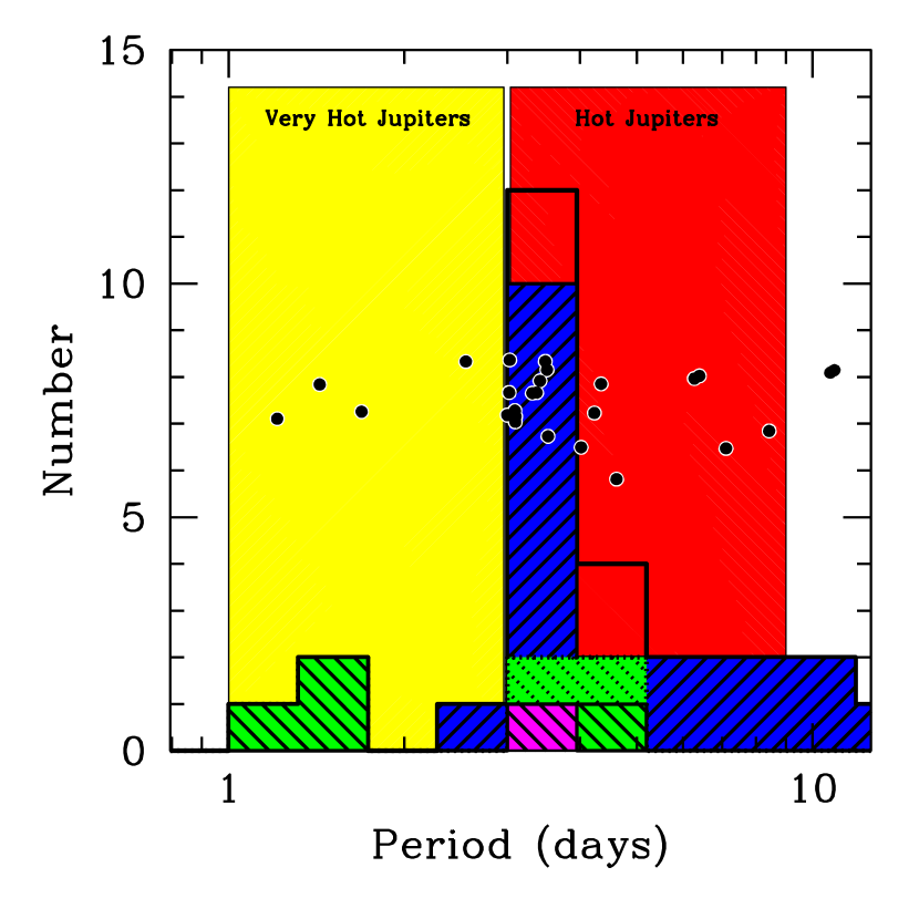
Figure 1.— The period distribution of short-period extrasolar giant planets. The blue shaded histogram shows planets with mass $M_{p}\sin i>0.2~{}M_{J}$ detected via radial velocity (RV) surveys, the green shaded histogram shows planets detected via the OGLE transit surveys, and the magenta histogram shows the planet detected via the TrES survey. The dotted green histogram shows the periods of the two unconfirmed candidate transiting planets with $P\gtrsim 3~{}\rm d$ (Konacki et al., 2003b). The unshaded histogram shows all planets. The yellow and red bands indicate the period ranges for our fiducial division into very hot Jupiters and hot Jupiters, respectively. The black points show the individual periods of the planets, the ordinate values are arbitrary.

RV surveys have so far been the most successful extrasolar planet detection technique. Recently, two other planet detection techniques have finally come to fruition, namely transit (TR) and microlensing surveys (Bond et al., 2004). In particular, RV follow-up of low-amplitude transits detected by the OGLE collaboration (Udalski et al., 2002a, b, c, 2003) has yielded four bona-fide planet detections (Konacki et al., 2003a; Bouchy et al., 2004; Konacki et al., 2004; Pont et al., 2004), and several strong candidates (Konacki et al., 2003b). Recently, the Trans-Atlantic Exoplanet Survey (TrES) collaboration announced the detection of a transiting planet around a relatively bright K0V star (Alonso et al., 2004). Figure 1 shows the period distribution of both the confirmed and candidate TR-detected planets, and Table 1 summarizes their properties. Notably, the first three planets detected via transits all have $P\simeq 1~{}\rm d$, considerably smaller than the periods of any planets detected via RV, and well below the pile-up and abrupt cutoff seen in the RV period distribution (see Figure 1). This is perhaps surprising because the sensitivity of RV surveys increases with decreasing period.

This apparent tension between the results of TR and RV surveys begs the question of whether the results from the two techniques are mutually consistent. In this paper we answer this question by considering a simple model for both the statistics and selection biases of the TR and RV surveys.

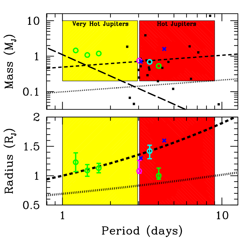
Figure 2.— Physical properties of short-period extrasolar planets. See Table 1 and references therein. Top Panel: The points show the mass $M_{p}$ (or $M_{p}\sin i$) of short-period planets in Jupiter masses ($M_{J}$) versus their period $P$ in days. Solid black points are RV-detected planets, green circles are confirmed TR-detected planets, blue crosses are candidate TR-detected planets, the cyan circle is the RV-detected transiting planet HD209458b, and the magenta circle is the bright transiting planet TrES-1. The dotted line line shows $M_{p}\sin i$ versus $P$ for an RV semi-amplitude of $K=20~{}{{\rm m\,s^{-1}}}$ for a planet in a circular orbit and a primary of $M=M_{\odot}$. We assume that RV surveys are complete above this limit, and therefore are complete to masses $M_{p}\sin i\geq 0.2M_{J}$ for $P\leq 9~{}\rm d$. The yellow and red bands indicate the period and mass ranges for our division into complete samples of very hot Jupiters and hot Jupiters, respectively. The short-dashed line corresponds to $K=100~{}{{\rm m\,s^{-1}}}$, roughly appropriate for the follow-up of fainter TR candidate planets. The long-dashed line shows the Roche limit for a planet with radius $R_{p}=2R_{J}$. Bottom Panel: The points show $R_{p}$ versus $P$ for known transiting planets and candidates. Symbol types are as in the top panel. The dashed line shows the contour of equal number of target stars in the effective TR survey volume, normalized to the number at $P=1~{}\rm d$ and $R_{p}=R_{J}$. The dotted line shows the lower limit on $R_{p}$ versus $P$ required to achieve a total signal-to-noise of ${\rm S/N}=9$, for typical light curves from the OGLE surveys. See text for details.

Table 1Parameters of Confirmed and Candidate Transiting Planets

Name	$P$ (days)	$a$ (AU)	$M_{p}$ ($M_{J}$)	$R_{p}$ ($R_{J}$)	$M_{*}$ ($M_{\odot}$)	$R_{*}$ ($R_{\odot}$)	$I$	$(V-I)$	$N_{tr}$	Reference
OGLE-TR-56	1.2119	0.023	$1.45\pm 0.23$	$1.23\pm 0.16$	$1.04\pm 0.05$	$1.10\pm 0.10$	15.30	1.26	11	1,2
OGLE-TR-113	1.4325	0.023	$1.08\pm 0.28$	$1.09\pm 0.10$	$0.79\pm 0.06$	$0.78\pm 0.06$	14.42	–	10	3,4
OGLE-TR-132	1.6897	0.031	$1.19\pm 0.13$	$1.13\pm 0.08$	$1.35\pm 0.06$	$1.43\pm 0.10$	15.72	–	11	3,5
OGLE-TR-111	4.0161	0.047	$0.53\pm 0.11$	$1.00_{-0.06}^{+0.13}$	$0.82_{-0.02}^{+0.15}$	$0.85_{-0.03}^{+0.10}$	15.55	–	9	6
OGLE-TR-10	3.1014	–	$0.70\pm 0.30$	1.3	–	–	14.93	0.85	4	7
OGLE-TR-58	4.34	–	$1.60\pm 0.80$	1.6	–	–	14.75	1.20	2	7
HD209458	3.5248	0.045	$0.69\pm 0.05$	$1.42_{-0.13}^{+0.10}$	$1.06\pm 0.13$	$1.18\pm 0.10$	–	–	–	8,9
TrES-1	3.0301	0.039	$0.75\pm 0.05$	$1.08_{-0.04}^{+0.18}$	$0.88\pm 0.07$	$0.85_{-0.05}^{+0.10}$	10.64	1.15	–	10

References. — (1) Konacki et al. 2003a; (2)Torres, Konacki, Sasselov, & Jha 2004; (3)Bouchy et al. 2004; (4)Konacki et al. 2004; (5) Moutou, Pont, Bouchy, & Mayor 2004; (6)Pont et al. 2004; (7)Konacki et al. 2003b; (8)Brown et al. 2001; (9)Cody & Sasselov 2002; (10)Alonso et al. 2004

2. A Simple Argument

In this section, we present a simple, straightforward argument for why we conclude that RV and TR surveys are essentially consistent. These arguments are presented in more detail in §3, §4, and the Appendix.

The primary difference between RV and transit surveys is in how their target stars are chosen. RV surveys are essentially ‘volume-limited,’ and thus have a fixed number of target stars in their sample. Because RV surveys have a fixed sample size, their relative sensitivity as a function of the mass and period depends only on the intrinsic sensitivity of the RV technique. This scales as $K\propto M_{p}\sin iP^{-1/3}$, where the semi-amplitude $K$ characterizes the signal strength. It is possible to define a complete sample of planets by considering an appropriate limit on $K$. RV surveys are expected to be essentially complete for $K\gtrsim 20~{}{\rm m~{}s^{-1}}$ (Tabachnik & Tremaine, 2002), which corresponds to $M_{p}\sin i>0.2~{}M_{J}$ and $P\lesssim 9~{}\rm d$ for solar-mass primaries and circular orbits. RV surveys indicate that the relative frequency of $1-3~{}\rm d$ planets to $3-9~{}\rm d$ planets in this complete sample is $\sim 0.07_{-0.04}^{+0.09}$, where the errors account for Poisson fluctuations (and are calculated in §4).

Field TR surveys, in contrast to RV surveys, are signal-to-noise (${\rm S/N}$) limited. As a result, the effective volume probed by TR surveys, and therefore the number of target stars, depends on the total signal-to-noise ratio of the transits, which in turn depends on the radius and period of the planets. The basic scaling of the sensitivity of TR surveys with period can be understood as follows. The flux $F$ of a star is $F\propto d^{-2}$, where $d$ is the distance to the star. The photometric error $\sigma\propto F^{-1/2}\propto d$. The number of data points $N_{p}$ during transits is proportional to the duty cycle, which is inversely proportional to the semi-major axis $a$. Thus $N_{p}\propto a^{-1}\propto P^{-2/3}$. The total signal-to-noise of a transiting planet is ${\rm S/N}\propto N_{p}^{1/2}\sigma^{-1}$ and thus, at fixed ${\rm S/N}$, $\sigma\propto N_{p}^{1/2}\propto P^{-1/3}$. Therefore, $d\propto P^{-1/3}$, i.e. the distance out to which one can detect a transiting planet at fixed signal-to-noise scales as $P^{-1/3}$. The number of stars in the survey volume is $\propto d^{3}\propto P^{-1}$. Combined with the transit probability, which scales as $a^{-1}\propto P^{-2/3}$, this implies an overall sensitivity $\propto P^{-5/3}$.

Thus, TR surveys are, on average, $\sim(1/3)^{-5/3}\sim 6$ times more sensitive to $P=1~{}\rm d$ planets than $P=3~{}\rm d$ planets. The observed relative frequency of confirmed $1-3~{}\rm d$ to $3-9~{}\rm d$ planets discovered in the OGLE TR surveys is $\sim 3$, which corresponds to an intrinsic relative frequency (after accounting for the factor of $6$) of $\sim 0.5_{-0.3}^{+1.5}$, as compared to $\sim 0.07_{-0.04}^{+0.09}$, for the RV surveys. Thus, considering the large errors due to small number statistics, RV and TR surveys are basically consistent (at better than the $\sim 2\sigma$ level). If at least one of the remaining OGLE $P\geq 3~{}\rm d$ planet candidates is confirmed in the future, then TR and RV surveys are consistent at better than $1\sigma$. In other words, there are not enough planets detected to robustly conclude that the RV and TR short period planet results are inconsistent.

As we discuss in more detail in the the Appendix, there are additional effects that favor the confirmation of shorter-period transiting planets. First, shorter-period planets will generally tend to exhibit more transits; this makes their period determinations from the TR data more accurate. Accurate periods aid significantly in RV follow-up and confirmation. Second, shorter-period planets will generally have larger velocity semi-amplitudes $K$, both because of their smaller periods $(K\propto P^{-1/3})$, and because there appears to be a dearth of massive ($M_{p}\sin i\gtrsim M_{J}$) planets with $P=3-9~{}\rm d$ (see Figure 2).

3. Selection Effects in Transit Surveys

In this section, we present a more detailed derivation of the sensitivity of signal-to-noise limited planet TR surveys as a function of the period and radius of the planet.

Field searches for transiting planets are very different from RV searches as they are uniform surveys, in which the target stars are all observed in the same manner (rather than targeted observations of individual stars). Therefore, the noise properties vary from star to star. As a result, the relative number of planets above a given ${\rm S/N}$ threshold depends not only on the way in which the intrinsic signal scales with planet properties, but also on the number of stars with a given noise level. Since, for transit surveys, the noise depends on the flux of the star, which depends on the distance to the star, the effective number of target stars depends on the number of stars in the effective survey volume that is defined by the maximum distance out to which a planet produces a ${\rm S/N}$ greater than the threshold. This leads to a strong sensitivity of TR surveys on planet period and radius (as well as parent star mass and luminosity, see Pepper, Gould, & Depoy 2003), which we now derive.

The total signal-to-noise of a transiting planet can be approximated as

$${\rm\frac{S}{N}}=N_{p}^{1/2}\left(\frac{\delta}{\sigma}\right).$$ (1)

Here $N_{p}$ is the total number of measurements during the transit, $\delta$ is the depth of the transit, and $\sigma$ is the fractional flux error for a single measurement. We can approximate $N_{p}=N_{\rm tot}(R_{*}/\pi a)$ (for a central transit) and $\delta=(R_{p}/R_{*})^{2}$. Here $N_{\rm tot}$ is the total number of observations, $a$ is the semi-major axis of the planet, and $R_{*}$ is the radius of the parent star. Combining these relations with Kepler’s third law, we have

$${\rm\frac{S}{N}}\propto P^{-1/3}R_{p}^{2}\sigma^{-1}$$ (2)

We then estimate the relative sensitivity as follows. Following Pepper, Gould, & Depoy (2003), the number of target stars for which a planet of a given $P$ and $R_{p}$ would produce a ${\rm S/N}$ greater than a given threshold is proportional to

$$\frac{{\rm d}^{2}{\cal N}(P,R_{p})}{{\rm d}P{\rm d}R_{p}}\propto f(P,R_{p})P_{T}(P)V_{\rm max}(P,R_{p}),$$ (3)

where $f(P,R_{p})\equiv{{\rm d}^{2}n(P,R_{p})}/{{\rm d}P{\rm d}R_{p}}$ is the intrinsic frequency of planets as a function of $P$ and $R_{p}$, $P_{T}(P)$ is the probability that a planet of a given $P$ will transit its parent star, and $V_{\rm max}(P,R_{p})$ is the maximum volume within which a planet of a given $P$ and $R_{p}$ can be detected. The geometric transit probability is simply $P_{T}\simeq R_{*}/a\propto P^{-2/3}$. We assume the form $V_{\rm max}\propto F_{\rm min}^{-3/2}$, where $F_{\rm min}(P,R_{p})$ is the minimum flux of a star around which a planet of period $P$ and radius $R_{p}$ can be detected; this form is appropriate for a constant volume density of stars and no extinction. For fixed ${\rm S/N}$, we have from equation (2) that $\sigma\propto P^{-1/3}R_{p}^{2}$. For source-dominated photon noise, $\sigma\propto F_{\rm min}^{-1/2}$, and so $F_{\rm min}\propto P^{2/3}R_{p}^{-4}$ and $V_{\rm max}\propto P^{-1}R_{p}^{6}$. Finally, combining this with $P_{T}\propto P^{-2/3}$, we find

$$\frac{{\rm d}^{2}{\cal N}}{{\rm d}P{\rm d}R_{p}}\propto f(P,R_{p})R_{p}^{6}P^{-5/3}.$$ (4)

This strong function of $P$ implies that the TR surveys are very biased toward detecting short-period planets.

Note that, in deriving equation (4), we have made the simplistic assumption that the number of data points during transit is proportional to the duty cycle, $N_{p}\propto R_{*}/\pi a$. This assumes random sampling and short periods as compared to the transit campaign. In fact, actual transit campaigns have non-uniform sampling and finite durations. In addition, transit candidates require RV follow-up for confirmation; this introduces additional selection effects. We consider both effects in detail in the Appendix.

4. Radial Velocity Versus Transits

We now address the question of whether the period distribution of the planets discovered by RV and TR surveys are consistent, considering both the selection biases discussed in the previous section, as well as the effects of small-number statistics.

For our fiducial comparisons, we consider two equal-width logarithmic bins in period with $(P_{1,\rm min},P_{1,\rm max})=(1\rm d,3\rm d)$ and $(P_{1,\rm min},P_{1,\rm max})=(3\rm d,9\rm d)$. We argued in §3 that local RV surveys should be essentially complete for planets with velocity semi-amplitude $K\gtrsim 20~{}{\rm m\,s^{-1}}$, and therefore if we restrict our analysis to $M_{p}\sin i\geq 0.2M_{J}$, then the observed number of planets detected by RV in these two bins should be an unbiased sample of the true distribution of planets (see Figure 2). We will also restrict our attention to $M_{p}\sin i\leq 10M_{J}$ to avoid possible brown dwarf candidates. The number of RV planets with $0.2M_{J}\leq M_{p}\sin i\leq 10M_{J}$ in our two fiducial period bins is given in Table 2. There is one planet in the first bin, and 15 in the second. Therefore the relative frequencies are $\sim 7\%$. We denote these two complete samples as “Very Hot Jupiters” (VHJ) and “Hot Jupiters” (HJ), respectively.

For comparison to the RV surveys, we will consider the results from the two campaigns by the OGLE collaboration. Pertinent details about the OGLE surveys are summarized in the Appendix. Because the OGLE searches are signal-to-noise limited surveys, as opposed to the volume-limited RV surveys, it is not possible to define a complete, unbiased sample of observed planets (see the discussion in §3), and we must take into account the selection biases to infer the true planet frequency. We first assume a frequency distribution $f(P,R_{p})$. We assume that planets are uniformly distributed in $\log{P}$ within each bin, and that all planets in bin $i$ have radius $R_{p,i}$. This gives an intrinsic frequency distribution of,

$$f_{i}(P,R_{p})=\frac{{\rm d}^{2}n_{i}(P,R_{p})}{{\rm d}P{\rm d}R_{p}}=\frac{N_{i}}{\Delta{\log P_{i}}}P^{-1}\delta_{\rm D}(R_{p}-R_{p,i})$$ (5)

where $N_{i}$ is the total number of planets in bin $i$, $\Delta{\log P_{i}}=\log P_{i,\rm max}-\log P_{i,\rm min}$ is logarithmic width of the bin, and $\delta_{\rm D}$ is the Dirac delta function. From equation 4, the expected number ${\cal N}_{i}$ of observed transiting planets in bin $i$ is,

$${\cal N}_{i}(P,R_{p})\propto\int{\rm d}R_{p}\int_{P_{i,\rm min}}^{P_{i,\rm max}}{\rm d}P\,f_{i}(P,R_{p})R_{p}^{6}P^{-5/3}.$$ (6)

The constant of proportionality is independent of $P$ and $R_{p}$, and thus the ratio of the observed number of planets in the two bins is simply,

$$\frac{{\cal N}_{1}}{{\cal N}_{2}}=r_{12}\left(\frac{R_{p,1}}{R_{p,2}}\right)^{6}\left(\frac{P_{1,\rm min}}{P_{2,\rm min}}\right)^{-5/3},$$ (7)

where we have assumed that $\Delta\log P_{1}=\Delta\log P_{2}$, and we have defined $r_{12}=N_{1}/N_{2}$, the ratio of the intrinsic number of planets in the two period bins, i.e. the relative frequency of VHJ and HJ.

For simplicity, we will assume that VHJ and HJ have similar radii on average, and so $R_{p,1}=R_{p,2}$. For our period bins, the last factor is $(1\rm d/3\rm d)^{-5/3}\sim 6$. The number of planets detected by TR surveys in the first bin is ${\cal N}_{1}=3$. There is one confirmed OGLE planet detected by TR in the second bin. This implies a intrinsic relative frequency of VHJ and HJ of $r_{12}\sim 50\%$, which is a factor of $\sim 7$ larger than inferred from RV surveys.

Given the relatively small number of planets in each of our two fiducial period bins, we must account for Poisson fluctuations in order to provide a robust estimate of the relative frequency $r_{12}$. In the limit of a large number of trials, the probability ${\cal P}$ of observing ${\cal N}$ planets given ${\cal M}$ expected planets is,

$${\cal P}({\cal N}|{\cal M})=\frac{e^{-{\cal M}}{\cal M}^{\cal N}}{{\cal N}!}.$$ (8)

For large ${\cal M}$, the probability of observing any particular value of ${\cal N}$ becomes small, simply because of the large number of possible outcomes. We therefore consider relative probabilities $\tilde{\cal P}({\cal N}|{\cal M})\equiv{\cal P}({\cal N}/{\cal M})/{\cal P}_{\rm max}({\cal M})$, and normalize ${\cal P}({\cal N}|{\cal M})$ by the maximum probability ${\cal P}_{\rm max}({\cal M})\equiv{\rm max}[{\cal P}(1|{\cal M}),{\cal P}(2|{\cal M}),...,{\cal P}(\infty|{\cal M})]$ for a given expected number ${\cal M}$.

We can now construct probability distributions ${\cal P}(r_{12}|{\cal N}_{1},{\cal N}_{2})$ of $r_{12}$, given the observed numbers ${\cal N}_{1}$ and ${\cal N}_{2}$ of VHJ and HJ, and incorporating selection biases and Poisson fluctuations. This probability is,

$${\cal P}(r_{12}|{\cal N}_{1},{\cal N}_{2})\propto\int{\rm d}{\cal M}_{1}\tilde{\cal P}({\cal N}_{1}|{\cal M}_{1})\tilde{\cal P}({\cal N}_{2}|{\cal M}_{2}),$$ (9)

here ${\cal M}_{2}$ depends on ${\cal M}_{1}$ and $r_{12}$. For RV, it is simply ${\cal M}_{2}={\cal M}_{1}/r_{12}$, whereas for TR, it is related via equation (7) (replacing ${\cal N}\rightarrow{\cal M}$). Note that, up to a constant, equation (9) is equivalent under the transposition ${\cal M}_{1}\leftrightarrow{\cal M}_{2}$, and we could have also integrated over ${\cal M}_{2}$.

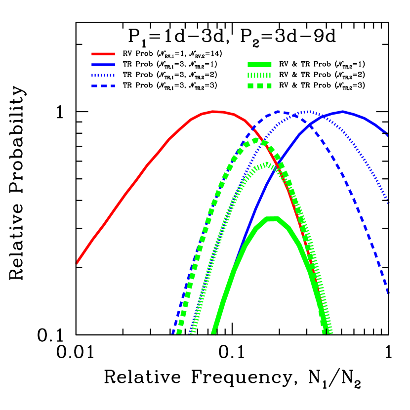
Figure 3.— The lines show the relative probability of observing ${\cal N}_{1}$ planets in the period range $P_{1}=$1d-3d and ${\cal N}_{2}$ planets in the period range $P_{1}=$3d-9d, for an absolute relative frequency of planets in these two period ranges of $r_{12}\equiv N_{1}/N_{2}$, and assuming a uniform logarithmic distribution in $P$ in each bin. The curves take into account both Poisson fluctuations and period-dependent selection biases. The red curve shows the probability corresponding to the RV surveys, which observe ${\cal N}_{{\rm RV},1}=1$ in the period range $P_{1}$=1d-3d and ${\cal N}_{{\rm RV},2}=15$ in the period range $P_{2}$=3d-9d. The blue curves are for the TR surveys, for ${\cal N}_{{\rm TR},1}=3$, and ${\cal N}_{{\rm TR},2}=1$ (solid), 2 (dotted), and 3 (dashed). The green curves are joint RV and TR probabilities, for ${\cal N}_{{\rm RV},1}=1$, ${\cal N}_{{\rm RV},2}=14$, ${\cal N}_{{\rm TR},1}=3$, and ${\cal N}_{{\rm TR},2}=1$ (solid), 2 (dashed), or 3 (dotted).

Table 2Radial Velocity versus Transits

Assumption	Range	# RV	# TR	Range	# RV	# TR	$N_{1}/N_{2}$	Prob.
Logarithmic	$P$=1d-3d	1	3	$P$=3d-9d	15	0	$0.21_{-0.09}^{+0.16}$	$12.7\%$
–	–	–	–	–	–	1	$0.18_{-0.08}^{+0.12}$	$33.1\%$
–	–	–	–	–	–	2	$0.15_{-0.07}^{+0.10}$	$54.1\%$
–	–	–	–	–	–	3	$0.13_{-0.05}^{+0.09}$	$70.9\%$
Logarithmic	$P$=1d-2d	0	3	$P$=2d-4d	11	0	$0.25_{-0.12}^{+0.21}$	$2.0\%$
–	–	–	–	–	–	1	$0.22_{-0.10}^{+0.18}$	$6.5\%$
–	–	–	–	–	–	2	$0.20_{-0.09}^{+0.14}$	$13.3\%$
–	–	–	–	–	–	3	$0.17_{-0.08}^{+0.12}$	$20.7\%$
Linear	$P$=1d-3d	1	3	$P$=3d-5d	12	1	$0.25_{-0.11}^{+0.18}$	$22.6\%$

Figure 3 shows the probability distribution for $r_{12}$, normalized to the peak probability, as inferred from RV and TR surveys, assuming that ${\cal N}_{2}=1,2$ or $3$ of the candidate TR planets with $P=3\rm d-9\rm d$ are real. The probability distributions peak at the expected value given the observed numbers of VHJ and HJ. However, due to Poisson fluctuations, the distributions are quite broad. For example, the RV surveys imply a median and 68% confidence interval of $r_{12}=0.07_{-0.04}^{+0.09}$, whereas the TR surveys with ${\cal N}_{{\rm TR},2}=1$ imply $r_{12}=0.5_{-0.3}^{+1.5}$. Therefore, it is clear that when Poisson fluctuations are taken into account, these two determinations are roughly consistent. Figure 3 also shows the product of the relative probabilities of $r_{12}$ from the RV and TR surveys. Considering the one confirmed $P\geq 3\rm d$ OGLE planet (${\cal N}_{{\rm TR},2}=1$), the median and 68% confidence interval for the joint probability distribution is $r_{12}=0.18_{-0.08}^{+0.12}$. The peak probability is $\sim 33\%$. Table 2 summarizes the inferred values and peak probabilities of $r_{12}$, including the cases ${\cal N}_{{\rm TR},2}=0,1,2,3$. Even if none of the $P>3~{}\rm d$ TR planets were real, the TR and RV surveys would still have been compatible at the $\sim 2\sigma$ level. We therefore conclude that the TR and RV surveys are consistent, and imply a relative frequency of VHJ to HJ of $\sim 10-20\%$, with the precise number and degree of consistency depending on how many of the $P>3~{}\rm d$ TR planets turn out to be real.

Two of the HJ in our sample orbit stars that are members of a binary system ($\tau$ Boo and $\upsilon$ And). There have been various studies that indicate that such planets may have properties that are statistically distinct from those of planets orbiting single stars (e.g., Eggenberger, Udry, & Mayor 2004). Since it is unclear whether planets orbiting stars that are members of a binary system could be detected in the OGLE surveys, it is interesting to redo the analysis above, excluding these two planets. We find that doing so leaves our conclusions unchanged. For example, we infer a relative frequency of $r_{12}=0.16^{+0.12}_{-0.07}$ for ${\cal N}_{{\rm TR},2}=2$, with a peak probability of $62\%$, as compared to $r_{12}=0.15_{-0.07}^{+0.10}$ and a peak probability of $54\%$ when we include these two planets.

If we include in our analysis planets with mass $M_{p}\sin i\leq 0.2M_{J}$ (and so the two new Neptune mass planets with $P<3~{}\rm d$, (Butler et al., 2004; McArthur et al., 2004)), as well as the newly-discovered bright transiting planet TrES-1 (Alonso et al., 2004) with $P=3.0301~{}\rm d$, RV and TR surveys imply relative frequencies of $0.16_{-0.08}^{+0.15}$ and $0.32_{-0.18}^{+0.46}$, respectively. In other words, the two types of surveys are highly consistent. Combining both surveys, we find a relative frequency of $0.20_{-0.08}^{+0.13}$, with a peak probability of $\sim 87\%$. We stress that including these planets is probably not valid, because (1) RV surveys are very incomplete for $M_{p}\sin i\lesssim 0.1~{}M_{J}$, (2) it is not at all clear that TR surveys could detect planets with mass as low as Neptune, (3) even if the TR surveys could detect such planets, they would be extremely difficult to confirm from follow-up RV measurements, and (4) the details of the TrES survey necessary for a proper statistical analysis are unknown. However, the fact that the relative frequency agrees with that inferred when these planets are not included demonstrates that our conclusions are fairly robust.

We have checked that changing the binning or the form of period distribution does not alter our conclusions substantially. For example, if we choose equal logarithmic bins of $1-2~{}\rm d$ and $2-4~{}\rm d$, the RV surveys imply a $1\sigma$ upper limit to the relative frequency of planets with $P=1-2~{}\rm d$ versus $2-4~{}\rm d$ of $0.2$. This is compared to a relative frequency of $1.1_{-0.7}^{+2.8}$ implied by TR surveys. In this case, TR and RV surveys are consistent at the $\sim 2\sigma$ level. Taken together, TR and RV surveys imply a relative frequency of $0.22_{-0.10}^{+0.18}$ for ${\cal N}_{{\rm TR},2}=1$, with a peak probability of $\sim 7\%$. For planets distributed linearly with period, and period bins of $1-3~{}\rm d$ and $3-5~{}\rm d$, we find a relative frequency of $0.25_{-0.11}^{+0.18}$ for ${\cal N}_{{\rm TR},2}=1$, with a peak probability of $\sim 23\%$. We have also checked that aliasing due to uneven sampling does not affect our results substantially. See the Appendix for more details.

5. Hidden Assumptions, Caveats and Complications

In this section, we briefly mention various caveats and complications that may affect our results in detail. We begin by making a list of some of the more important hidden assumptions we have made. For completeness, we also list assumptions that we have already addressed.

1. ${\rm S/N}$-limited TR Surveys: We have assumed that the detection of planets in the OGLE surveys is limited only by ${\rm S/N}$, and not by, e.g. apparent magnitude. In other words, all stars for which planets (with the periods and radii we consider) would produce transits with ${\rm S/N}>9$ are considered. We discuss the validity of this assumption in more detail below.

2. Uniform Sampling: For the majority of our results, we have assumed uniform sampling.

3. Logarithmic Period Distribution and Specific Binning: For the majority of our results, we have assumed a logarithmic intrinsic period distribution, and specific choice of bins of $P=1-3~{}\rm d$ and $P=3-9~{}\rm d$.

4. All Detected Planets Can Be Confirmed: We have implicitly assumed that all planets detected in TR surveys can be confirmed via follow-up RV observations, regardless of their period. Because of the prevalence of false positives that mimic planetary transit signals, it is not possible to use the observed relative frequency of planet candidates as a function of period to infer the the true frequency, one must instead use the observed frequency of true planets, as confirmed by follow-up RV observations.

5. Homogeneous Stellar Populations: We have assumed that the population of source stars does not vary as a function of distance, and therefore that terms in the transit sensitivity that depend on the mass, radius, and luminosity of the host stars drop out.

6. Uniform Stellar Density: We adopted $V_{\rm max}\propto F_{\rm min}^{-3/2}$, which is assumes a constant volume density of stars and no dust.

7. Uniform Intrinsic Period Distribution: We have assumed that the period distribution of planets is uniform (either in log or linear period). It is clear, given the ‘pile-up’ of planets at $P\sim 3~{}\rm d$, that this assumption cannot be correct in detail.

8. Photon and Source Limited Noise: We assumed that the photometric precision is photon-noise limited (i.e. no systematic errors), and furthermore dominated by the source (i.e. sky noise is negligible).

9. Correspondence Between Detectable RV and TR Planets: We have assumed that all planets in the ‘complete’ sample from RV surveys are detectable in TR surveys, i.e. that both surveys probe the same population of planets.

10. Constant Radii: We have assumed that VHJ and HJ have equal, constant radii.

11. No Correlation Between Planet and Stellar Properties: We have assumed that the physical properties of short-period planets are uncorrelated with the physical properties of their parent stars.

The first assumption, namely that the OGLE TR surveys are ${\rm S/N}$-limited, is the most crucial, as it provides the crux of our argument that transit surveys are much more sensitive to short period planets than long period planets. In fact, the OGLE surveys are not strictly ${\rm S/N}$-limited, as several cuts were imposed to preselect light curves to search for transiting planets. Of the cuts made, the most relevant here was the exclusion of light curves whose root-mean-squared (RMS) scatter exceeded 1.5%. This is important because it effectively limits the volume which is searched for planets, in a way that depends on the period and radius of the planet. If this volume is smaller than the largest volume for which the ${\rm S/N}$ is greater than the threshold, then the survey is no longer ${\rm S/N}$-limited. From the definition of the ${\rm S/N}$ (Eq. 1), and assuming that the maximum photometric error $\sigma_{\rm max}$ is equal to the maximum RMS, we find that the TR surveys are ${\rm S/N}$-limited provided that the ratio of planet radius to stellar radius satisfies,

$$\frac{R_{p}}{R_{*}}\leq\left(\frac{\rm S}{\rm N}\right)^{1/2}\left(\frac{\sigma_{\rm max}}{N_{\rm tot}^{1/2}}\right)^{1/2}\left(\frac{P^{2}\pi GM_{*}}{4R_{*}^{3}}\right)^{1/12}.$$ (10)

For $\sigma_{\rm max}=1.5\%$ and a threshold of ${\rm S/N}=9$,

$$\frac{R_{p}}{R_{*}}\leq 0.12\left(\frac{P}{1\rm d}\right)^{1/6}\left(\frac{M_{*}}{M_{\odot}}\right)^{1/12}\left(\frac{R_{*}}{R_{\odot}}\right)^{-1/4}\left(\frac{N_{\rm tot}}{10^{3}}\right)^{-1/4}.$$ (11)

For the 2002 OGLE campaign, $N_{\rm tot}=1166$. This gives for $M_{*}=M_{\odot}$, $R_{*}=R_{\odot}$, and $P=1~{}\rm d$ (the smallest period we consider) $R_{p}/R_{*}\lesssim 0.12$. Therefore, for solar-type primaries, TR surveys are not ${\rm S/N}$-limited for the largest planets and smallest periods, and the arguments we have presented that are based on this assumption will break down. In practice, the magnitude of the correction will depend on the size distribution of planet radii, as well as the distribution of primary radii. However, if planets with $R_{p}/R_{*}\geq 0.12$ are relatively rare, then the correction will generally be small. We note that the sensitivity of TR surveys to planets around small primaries can be severely reduced by imposing magnitude or RMS limits, and thus future transit searches should take care when making such cuts that they are not rejecting otherwise viable candidates.

We have discussed the effects of our second, third, and fourth assumptions on our results in §4 and the Appendix. Although violations of these can and do affect our results in detail, they do not change our basic conclusions substantially.

Violations of the remaining assumptions will have various effects on our conclusions, however investigation of these in detail is well beyond the scope of the paper. Furthermore, although the importance of many of these assumptions can be determined directly from data, these data are not presently available. In the end, however, our assumptions are approximately valid, and a more careful examination of these issues is not warranted, given the small number of detected planets and resulting poor statistics. Our primary goal is to provide general insight into the biases and selection effects inherent in RV and (especially) TR surveys. We note that, when many more planets are detected and the present analysis revisited, the assumptions listed above will likely have to be reconsidered more carefully.

6. Discussion

We have demonstrated that the sensitivity of signal-to-noise limited transit surveys scales as $P^{-5/3}$. This strong dependence on $P$ arises from geometric and signal-to-noise considerations, and implies that transit surveys are $\sim 6$ times more sensitive to $P=1~{}\rm d$ planets than $P=3~{}\rm d$ planets. When these selection biases and small number statistics are properly taken into account, we find that the populations of close-in massive planets discovered by RV and TR surveys are consistent (at better than the $2\sigma$ level). In other words, there are not enough planets detected to robustly conclude that the RV and TR short-period planet results are inconsistent. We then used the observed relative frequency of planets as a function of period as probed by both methods to show that the HJ are approximately 5-10 times more common that VHJ.

RV surveys have demonstrated that the absolute frequency of HJ is $\sim 1\%$ (Marcy et al., 2003), and thus the frequency of VHJ is $\sim 0.1-0.2\%$, i.e. 1 in 500-1000 stars have a VHJ. The frequency of VHJ is approximately the same as the frequency of transiting HJ, and therefore future RV surveys that aim to detect short-period planets by monitoring a large number of relatively nearby stars over short time periods (Fischer et al., 2004) should detect VHJ at approximately the same rate as transiting planets. Should such RV surveys not uncover VHJ at the expected rate, this would likely point to a difference in the populations of planetary systems probed by RV and TR surveys.

Roughly $15\%$ of VHJ should transit their parent stars, as opposed to $\sim 7\%$ of HJ, and approximately one in 3300-6700 single main sequence FGK stars should have a transiting VHJ, as opposed to one in 1400 for HJ. It has been estimated that there are $\sim 30$ detectable transiting HJ around stars with $V\lesssim 10$ in the entire sky (Pepper, Gould, & Depoy, 2003; Deeg et al., 2004), and thus $\sim 7-13$ transiting VHJ. The detection of only $3$ VHJ in the OGLE surveys containing $\sim 150,000$ stars implies that only $5-10\%$ of the sources are single, main-sequence, FGK stars useful for detecting transiting planets, roughly in accord with, but somewhat smaller than, the fraction estimated for TR surveys of brighter stars (Brown, 2003). The fact that other deep surveys such as EXPLORE (Mallén-Ornelas et al., 2003) have not detected any promising VHJ candidates despite searching a similar number of stars may be due to either small number statistics, reduced efficiency due to shorter observational campaigns, or both. Finally, we estimate that Kepler should find $\sim 15-30$ transiting VHJ around the $\sim 10^{5}$ main-sequence stars in its field-of-view.

It is interesting to note that there is some evidence that VHJ and HJ also appear to differ in their mass. Figure 2 shows the distribution of confirmed and candidate planets in the mass-period and radius-period plane. While there is a paucity of high-mass ($M_{p}\gtrsim M_{J}$) planets with periods of $P\sim 3-10~{}\rm d$ (Pätzold & Rauer, 2002; Zucker & Mazeh, 2002), all of the planets with $P\lesssim 3~{}\rm d$ have $M\geq M_{J}$. This includes the RV planet HD 73256b with $P=2.5~{}\rm d$, which argues that this planet is indeed a VHJ, and thus that RV surveys have already detected an analog to the OGLE short-period planets. The lack of high-mass HJ is certainly real, and thus the mere existence of VHJ with $M\geq M_{J}$ points toward some differentiation in the upper mass limit of the two populations. Whether or not the lack of lower-mass $0.5M_{J}\lesssim M_{p}\lesssim M_{J}$ VHJ is real is certainly debatable. For TR-selected planets, this could in principle be a selection effect if the radius is a strong decreasing function of decreasing mass in this mass range, however this is neither seen for the known planets with measured radii, nor is expected theoretically. RV follow-up would likely prove more difficult for such lower-mass objects, however (see Figure 2).

As can be seen in Figure 2, there appears to be an ‘edge’ in the distribution of planets in the mass-period plane that is reasonably well-described by twice the Roche limit for a planet radius of $R=R_{J}$. This has been interpreted as evidence that short period planets may have originated from highly-eccentric orbits, which underwent strong tidal evolution with their parent stars, leading to circularization at twice the Roche limit (Faber, Rasio, & Willems, 2004). However, this model alone cannot explain the pile-up at 3 days and paucity of VHJ relative to HJ. Alternatively, it may be that massive $M\geq M_{J}$ planets were not subject to whatever mechanism halted the migration of less massive planets at periods of $P\simeq 3~{}\rm d$. Rather, these massive planets migrated on quasi-circular orbits while they were still young (and thus relatively large, $\sim 2R_{J}$), through periods of $3~{}\rm d$, until they reached their Roche limit, at which point they may have lost mass and angular momentum to their parent star, halting their inward migration (e.g. Trilling et al. 1998).

The recently-discovered short-period Neptune-mass planets (Santos et al., 2004; McArthur et al., 2004; Butler et al., 2004) complicate the interpretation of the properties of short-period planets even further. Two of these planets have periods that are less than the $3~{}\rm d$ limit observed for planets with mass $0.2-1~{}M_{J}$. Both of these planets show marginal ($\sim 2\sigma$) evidence for non-zero eccentricity. In addition, 55 Cnc has a more distant companion with $P=14.653~{}\rm d$ (McArthur et al., 2004), and the RV curve for GJ 436b has marginal evidence for a linear trend, consistent with a more distant companion. Since tidal torques would be expected to circularize the orbits of such close planets on an extremely short time scale, this may be evidence for dynamical interactions with more distant companions, which may affect their migration and explain why they do not obey the $3~{}\rm d$ migration limit. However, we stress that the evidence for non-zero eccentricity in these planets is marginal, and thus will need to be confirmed with additional observations before any firm conclusions can be drawn. The fact that these planets have orbits that are smaller than the Roche edge observed for higher-mass planets is understandable if they are primarily rocky in composition.

It is clear that much remains to be understood about short period extrasolar planetary companions. In this regard, building statistics is essential. Future RV surveys that tailor their observations to preferentially discover large numbers of short-period planets are very important, and are currently being undertaken (Fischer et al., 2004). Complementarity is also essential: the success of TR surveys in uncovering a population of heretofore unknown planets demonstrates the benefit of searching for planets with multiple methods, each of which have their own unique set of advantages, drawbacks, and biases. In addition to the success of OGLE and TrES, all-sky shallow TR surveys (Deeg et al., 2004; Pepper, Gould, & Depoy, 2004; Bakos et al., 2004), wide-angle field surveys (Kane et al., 2004; Brown & Charbonneau, 2000), deep ecliptic surveys (Mallén-Ornelas et al., 2003), and surveys in stellar systems (Mochejska et al., 2002; Burke et al., 2003; Street et al., 2003; von Braun et al., 2004) should all uncover a large number of short-period planets which can be compared and combined with the yield of RV surveys to provide diagnostic ensemble properties of short-period planets.

Note: After the original submission of this paper, and during the refereeing process, we learned of several new results that bear on the discussion here. Bouchy et al. (2005) report on their follow-up of OGLE bulge candidates. They argue that OGLE-TR-58, listed as a possible planet candidate by Konacki et al. (2003b), is more likely a false positive caused by intrinsic stellar photometric variability. They also report radial velocity measurements of OGLE-TR-10 that indicate a possible planetary companion, in agreement with sparser RV data from Konacki et al. (2003b). Very recently, Konacki et al. (2005) report additional RV measurements of OGLE-TR-10, confirming the planetary nature of its companion, which has a radius $R_{p}=1.24\pm 0.09R_{J}$, and a mass $M_{p}=0.57\pm 0.12M_{J}$. The mass of this planet is consistent with other HJ, and significantly less than that of the known VHJ, reinforcing the case for a difference in the mass of these two populations of planets. With the confirmation of OGLE-TR-10, the number of HJ discovered in the OGLE transit surveys is ${\cal N}_{{\rm TR},2}=2$. If no other planets are uncovered from the first two OGLE campaigns, this implies a relative frequency of VHJ to HJ of $r_{12}=0.15_{-0.07}^{+0.10}$, with a peak probability of $\sim 54\%$. In other words, RV and TR surveys are consistent at better than the $1\sigma$ level.

Appendix A Properties of the OGLE Campaigns

In this paper, we have focused on the OGLE TR surveys, and we briefly summarize their properties here. OGLE mounted two separate campaigns toward the Galactic bulge and disk. In 2001, OGLE monitored 3 fields toward the Galactic bulge over a period of $45\rm d$, with $793$ epochs per field taken on $\sim 32$ nights. Approximately 52,000 disk stars with RMS $<1.5\%$ light curves were searched for low-amplitude transits, yielding a total of $64$ candidates (Udalski et al., 2002a, b). Of these candidates, one planetary companion was confirmed with radial velocity follow-up (OGLE-TR-56, Konacki et al. 2003a), and an additional two are planet candidates with significant spectroscopic follow-up (OGLE-TR-10 and OGLE-TR-58, Konacki et al. 2003b). In 2002, OGLE monitored an additional three fields in the Carina region of the Galactic disk over a period of $95~{}\rm d$, with $\sim 1166$ epochs per field taken on $\sim 76$ nights. Approximately 103,000 stars with RMS $<1.5\%$ light curves were searched for low-amplitude transits, yielding a total of $73$ candidates (Udalski et al., 2002c, 2003). Of these candidates, three planetary companions have been confirmed with radial velocity follow-up (OGLE-TR-111, OGLE-TR-113, and OGLE-TR-132, Bouchy et al. 2004; Konacki et al. 2004; Pont et al. 2004).

For both the 2001 and 2002 campaigns, candidates were found using the BLS algorithm of (Kovács, Zucker, & Mazeh, 2002). This method works by folding light curves about a trial period, and efficiently searching for dips in the folded curves that have a ${\rm S/N}$ larger than a given threshold. Udalski et al. (2002b, c, 2003) adopted a threshold of ${\rm S/N}=9$. Figure 2 shows a contour of ${\rm S/N}=9$ in the $(R_{p},P)$ plane, assuming $N_{\rm tot}=1166$ (as appropriate to the 2002 campaign), and $\sigma=0.005$, $R_{*}=R_{\odot}$, and $M_{*}=M_{\odot}$, as is typical of the OGLE target stars.

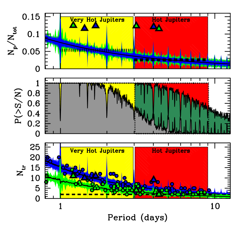
Figure 4.— Top Panel: The solid black line shows the mean fraction of data points in transit, $N_{p}/N_{\rm tot}$, as a function of period $P$ for the OGLE transit (TR) surveys, averaged over all phases. The green and blue shaded regions show the dispersion around the mean for the 2001 and 2002 OGLE campaigns, respectively. The yellow and red bands indicate the period and mass ranges for our division into very hot Jupiters and hot Jupiters, respectively. The dotted and dashed horizontal lines show the fraction of data points averaged over these two bins, assuming a uniform logarithmic distribution in $P$. The points show the periods of the OGLE TR confirmed and candidate planets; the ordinate values are arbitrary. Green and blue points are those found in the 2001 and 2002 campaigns, respectively. Middle Panel: The green shaded curve shows the probability, averaged over phase, for a planet with radius $R_{p}=0.1R_{*}$ to have ${\rm S/N}>9$ for a photometric precision $\sigma_{1}=0.005$, for the 2002 OGLE campaign. The red box shows the naive expectation under uniform sampling that all planets with $P\lesssim 9\rm d$ will have ${\rm S/N}>9$ for this $\sigma<\sigma_{1}$. The grey curve shows the same probability for $\sigma_{1}=3^{1/3}\sigma_{2}\sim 0.007$; three times more stars have $\sigma<\sigma_{2}$ than $\sigma<\sigma_{1}$. The yellow box shows the naive expectation that all planets with $P\lesssim 3\rm d$ will have ${\rm S/N}>9$ for $\sigma<\sigma_{2}$. Bottom Panel: The black lines show the number of observed transits, $N_{tr}$, with more than three points for the given $P$ averaged over all phases. The green and blue shaded regions show the dispersion around the mean for the 2001 and 2002 OGLE campaign, respectively. The points show the number of observed transits as a function of period for all the OGLE low-luminosity or planetary transit candidates. Green and blue points are those found in the 2001 and 2002 campaigns, respectively. Circles show all candidates, triangles are the confirmed planets or strong candidates. The horizontal bar shows $N_{tr}=2$, the minimum number of transits needed to establish a period.

Appendix B Uneven Sampling and Finite Campaign Duration

In evaluating the relative sensitivity of transit surveys, we made the simplistic assumption that the number of data points during transit is proportional to the transit duty cycle for a central transit, $N_{p}=R_{*}/\pi a$. This assumes random sampling and short periods as compared to the transit campaign. Of course, the OGLE campaigns have sampling that is far from random, and in addition have finite durations of 1-3 months. This introduces two effects. First, the true fraction of points in transit for an ensemble of light curves may be biased with respect to the naive estimate of $N_{p}/N_{\rm tot}=R_{*}/\pi a$. In addition, $N_{p}/N_{\rm tot}$ will depend strongly on phase, and thus an ensemble of systems at fixed $P$ will have a large dispersion in $N_{p}/N_{\rm tot}$.

We illustrate the effects of the non-uniform sampling and finite duration of the OGLE campaigns by analyzing the actual time stream of one light curve from each of the 2001 and 2002 campaigns, namely OGLE-TR-56 and OGLE-TR-113. We fold each of these light curves about a range of trial periods. For each $P$, we choose a random phase, and determine $N_{p}/N_{\rm tot}$ assuming a primary of $M=M_{\odot}$ and $R=R_{\odot}$. We repeat this for many different phases, and determine the mean and dispersion of $N_{p}/N_{\rm tot}$. The result is shown in Figure 4. The mean agrees quite well with the naive estimate of $N_{p}/N_{\rm tot}=R_{*}/\pi a$. However, the dispersion is significant, with $\sigma_{N_{p}}/N_{p}$ ranging from $\sim 20\%$ for $P\sim 1\rm d$ to $\sim 70\%$ for $P\sim 10\rm d$. Since ${\rm S/N}\propto N_{p}^{1/2}$, this translates to a dispersion in ${\rm S/N}$ of $\sim 0.5(\sigma_{N_{p}}/N_{p})\sim 10\%-35\%$. This implies that, for a small number of samples (as is the case here), the value of $N_{p}$ as a function of $P$ can have large stochastic variations about the naive analytic estimate. Such variations are largest for near-integer day periods, as can by seen in Figure 4.

The dispersion in the number of points during transit $N_{p}$ due to aliasing implies that the there is no longer a sharp cutoff in the distance out to which one can detect a planet of a given period. This is illustrated in the middle panel of Figure 4, where we plot the probability (averaged over phase) that a planet with a fractional depth $\delta=0.01$ will yield a ${\rm S/N}>9$ as a function of $P$ for the 2002 campaign, assuming a photometric precision of $\sigma=0.005$ (green shaded curve). Naively, the uniform sampling approximation would imply that for a ${\rm S/N}=9$ threshold all planets should be detectable out to a period of $P\sim 9\rm d$, and none with greater periods. In fact, due to the dispersion in $N_{p}$ for fixed period caused by aliasing, the transition is more gradual, such that it is possible to detect planets with $P>9~{}\rm d$, and there are sharp dips in the completeness near integer day periods. Figure 4 also shows the results for $\sigma=3^{-1/3}0.005\sim 0.007$ (grey shaded curve). There should be three times more stars with $\sigma=0.007$ than $\sigma=0.005$, and the naive expectation is that all planets with periods $P\lesssim 3\rm d$ should be detectable. Clearly uneven sampling will affect the estimates of the relative sensitivity of TR surveys as a function of period.

We note that OGLE-TR-111, which has $\delta\simeq 0.014$, $\sigma\sim 0.005$, and $P\simeq 4~{}\rm d$, would easily have exceeded the ${\rm S/N}>9$ cut even under the assumption of uniform sampling, which would predict ${\rm S/N}\sim 16$. Therefore, we find that it may not be necessary to invoke aliasing to explain the detection of this planet, as suggested by Pont et al. (2004). However, it is difficult to be definitive, because the ‘by-eye’ final selection of OGLE candidates may effectively impose a ${\rm S/N}$ limit that is significantly greater than the limit of ${\rm S/N}>9$ used for the initial candidate selection. The fact that a larger number of transits ($N_{tr}=9$) were detected for OGLE-TR-111 than would be expected based on its period is likely a consequence of its near-integer period.

We can make a rough estimate of the possible error made in adopting the naive estimate in the present case by determining the expected distribution in the total number of points in transit $N_{p}$. We consider our two fiducial period bins, $P_{1}=1-3\rm d$ and $P_{2}=3-9\rm d$, with planets distributed uniformly in $\log P$ within each bin. We then draw three planets from each bin, with a random phase and period for each planet. We evaluate $N_{p}$ for each, and then find the mean $\left<N_{p}\right>$ of the three planets. We repeat this for many different realizations. The ratio of the average $N_{p}$ for the two bins should be, on average, $\left<N_{p}\right>_{1}/\left<N_{p}\right>_{2}\simeq(1\rm d/3\rm d)^{-2/3}\sim 2$. For the 2001 campaign, we find a median and $95\%$ confidence interval of $\left<N_{p}\right>_{1}/\left<N_{p}\right>_{2}=2.11_{-1.06}^{+3.06}$, whereas for the 2002 campaign, we find $\left<N_{p}\right>_{1}/\left<N_{p}\right>_{2}=2.10_{-0.89}^{+1.83}$. A significant fraction of the variance arises from the small number of samples; if we assume there is no dispersion of the relation between $N_{p}$ and $P$ (i.e. uniform sampling), we find $\left<N_{p}\right>_{1}/\left<N_{p}\right>_{2}=2.08_{-0.52}^{+0.69}$. If we assume the exact periods for the four confirmed planets and two candidates, rather than random periods, we find very similar results, with $\left<N_{p}\right>_{1}/\left<N_{p}\right>_{2}=1.87_{-0.67}^{+1.42}$ for the 2001 campaign, and $\left<N_{p}\right>_{1}/\left<N_{p}\right>_{2}=1.92_{-0.77}^{+1.09}$ for the 2002 campaign.

By incorporating these distributions of $\left<N_{p}\right>_{1}/\left<N_{p}\right>_{2}$ into the analysis presented in §4, it is possible to determine the effect of aliasing on the inferred relative frequency of VHJ to HJ. We find that aliasing does not alter our conclusions substantially.

Appendix C Radial Velocity Follow-up Biases

One important distinction of TR surveys from RV surveys is that candidate transiting planets must be confirmed by RV measurements. Additional selection effects can be introduced at this stage. We discuss two such effects here.

The first effect is related to the detectability of the RV variations. The detectability depends on the flux of the source and the magnitude of the RV signal. At fixed transit depth, shorter-period planet candidates are, on average, fainter than longer-period candidates, since $F_{\rm min}\propto P^{2/3}$. For photon-limited measurements, the typical RV error is $\sigma_{\rm RV}\propto F_{\rm min}^{-1/2}\propto P^{-1/3}$. Thus, shorter period planets will therefore require longer integration times to achieve a fixed $\sigma_{\rm RV}$. However, the RV signal varies as $K\propto M_{p}P^{-1/3}$, and therefore, for all else equal, the dependence of the relative signal-to-noise ${\rm S/N}=K/\sigma_{K}$ on period cancels out. Thus, for fixed observing conditions, the relative ${\rm S/N}$ of RV measurements for VHJ versus HJ depends (on average) only on their masses. As discussed in §6, it appears that the upper mass threshold of VHJ and HJ are different: whereas there exists a real paucity of HJ with mass $\gtrsim M_{J}$, the four known VHJs all have masses $\gtrsim M_{J}$. This favors the confirmation of VHJs.

An additional bias arises because two or more transits are needed to establish the period of the planet. Since an accurate period is generally required for follow-up (because prior knowledge of the planet phase is important for efficient targeted RV observations), and longer periods are less likely to exhibit multiple transits, this bias also favors the confirmation of short-period planets. Figure 4 shows the mean and dispersion of the number of transits with more than three data points per transit as a function of period for the 2001 and 2002 OGLE campaign. The majority of planets with periods of $P\lesssim 3\rm d$ will exhibit at least two transits, whereas planets with $P\gtrsim 3\rm d$ are increasingly likely to exhibit only one transit (or no transits at all).

In summary, biases involved in both detection and confirmation of transiting planets generally favor short-period planets. It is important to stress that all of the above arguments are true only on average. For the handful of planets currently detected, stochastic effects associated with the small sample size change the magnitude or even sign of the biases.

References

- Alonso et al. (2004) Alonso, R., et al. 2004, ApJ, 613, L153
- Bakos et al. (2004) Bakos, G., Noyes, R. W., Kovács, G., Stanek, K. Z., Sasselov, D. D., & Domsa, I. 2004, PASP, 116, 266
- Bond et al. (2004) Bond, I. A., et al. 2004, ApJ, 606, L155
- Bouchy et al. (2004) Bouchy, F., Pont, F., Santos, N. C., Melo, C., Mayor, M., Queloz, D., & Udry, S. 2004, A&A, 421, L13
- Bouchy et al. (2005) Bouchy, F., Pont, F., Melo, C., Santos, N. C., Mayor, M., Queloz, D., & Udry, S. 2005, A&A, accepted (astro-ph/0410346)
- Brown et al. (2001) Brown, T. M., Charbonneau, D., Gilliland, R. L., Noyes, R. W., & Burrows, A. 2001, ApJ, 552, 699
- Brown (2003) Brown, T. M. 2003, ApJ, 593, L125
- Brown & Charbonneau (2000) Brown, T. M. & Charbonneau, D. 2000, ASP Conf. Ser. 219: Disks, Planetesimals, and Planets, 584
- Burke et al. (2003) Burke, C. J., Depoy, D. L., Gaudi, B. S., & Marshall, J. L. 2003, ASP Conf. Ser. 294: Scientific Frontiers in Research on Extrasolar Planets, 379
- Butler et al. (2004) Butler, P., Vogt, S. S., Marcy, G. W., Fischer, D. A., Wright, J. T., Henry, G. W., Laughlin, G., & Lissauer, J. 2004, ArXiv Astrophysics e-prints, astro-ph/0408587
- Cody & Sasselov (2002) Cody, A. M. & Sasselov, D. D. 2002, ApJ, 569, 451
- Deeg et al. (2004) Deeg, H. J., Alonso, R., Belmonte, J. A., Alsubai, K., Horne, K., & Doyle, L. R. 2004, PASP, 116, 985
- Eggenberger, Udry, & Mayor (2004) Eggenberger, A., Udry, S., & Mayor, M. 2004, A&A, 417, 353
- Faber, Rasio, & Willems (2004) Faber, J. A., Rasio, F. A., & Willems, B. 2004, (astro-ph/0407318)
- Fischer et al. (2004) Fischer, D., et al. 2004, ApJ, submitted (astro-ph/0409107)
- Kane et al. (2004) Kane, S. R., Collier Cameron, A., Horne, K., James, D., Lister, T. A., Pollacco, D. L., Street, R. A., & Tsapras, Y. 2004, MNRAS, 278
- Konacki et al. (2003a) Konacki, M., Torres, G., Jha, S., & Sasselov, D. D. 2003a, Nature, 421, 507
- Konacki et al. (2003b) Konacki, M., Torres, G., Sasselov, D. D., & Jha, S. 2003b, ApJ, 597, 1076
- Konacki et al. (2004) Konacki, M., et al. 2004, ApJ, 609, L37
- Konacki et al. (2005) Konacki, M., et al. 2005, ApJ, submitted (astro-ph/0412400)
- Kovács, Zucker, & Mazeh (2002) Kovács, G., Zucker, S., & Mazeh, T. 2002, A&A, 391, 369
- Mallén-Ornelas et al. (2003) Mallén-Ornelas, G., Seager, S., Yee, H. K. C., Minniti, D., Gladders, M. D., Mallén-Fullerton, G. M., & Brown, T. M. 2003, ApJ, 582, 1123
- Marcy et al. (2003) Marcy, G., Butler, P., Fischer, D., & Vogt, S. 2003, ASP Conf. Series, Extrasolar Planets: Today and Tomorrow
- Mayor et al. (2004) Mayor, M., Udry, S., Naef, D., Pepe, F., Queloz, D., Santos, N. C., & Burnet, M. 2004, A&A, 415, 391
- McArthur et al. (2004) McArthur, B. E., et al. 2004, ApJ, 614, L81
- Mochejska et al. (2002) Mochejska, B. J., Stanek, K. Z., Sasselov, D. D., & Szentgyorgyi, A. H. 2002, AJ, 123, 3460
- Moutou, Pont, Bouchy, & Mayor (2004) Moutou, C., Pont, F., Bouchy, F., & Mayor, M. 2004, A&A, 424, L31
- Pätzold & Rauer (2002) Pätzold, M. & Rauer, H. 2002, ApJ, 568, L117
- Pepper, Gould, & Depoy (2003) Pepper, J., Gould, A., & Depoy, D. L. 2003, Acta Astronomica, 53, 213
- Pepper, Gould, & Depoy (2004) Pepper, J., Gould, A., & Depoy, D. L. 2004, AIP Conference Series, 713, 185
- Pont et al. (2004) Pont, F., Bouchy, F., Queloz, D., Santos, N., Melo, C., Mayor, M., & Udry, S. 2004, A&A, 426, L15
- Santos et al. (2004) Santos, N. C., et al. 2004, (astro-ph/0408471)
- Street et al. (2003) Street, R. A., et al. 2003, MNRAS, 340, 1287
- Tabachnik & Tremaine (2002) Tabachnik, S. & Tremaine, S. 2002, MNRAS, 335, 151
- Torres, Konacki, Sasselov, & Jha (2004) Torres, G., Konacki, M., Sasselov, D. D., & Jha, S. 2004, ApJ, 609, 1071
- Trilling et al. (1998) Trilling, D. E., Benz, W., Guillot, T., Lunine, J. I., Hubbard, W. B., & Burrows, A. 1998, ApJ, 500, 428
- Udalski et al. (2002a) Udalski, A., et al. 2002a, Acta Astronomica, 52, 1
- Udalski et al. (2002b) Udalski, A., Zebrun, K., Szymanski, M., Kubiak, M., Soszynski, I., Szewczyk, O., Wyrzykowski, L., & Pietrzynski, G. 2002a, Acta Astronomica, 52, 115
- Udalski et al. (2002c) Udalski, A., Szewczyk, O., Zebrun, K., Pietrzynski, G., Szymanski, M., Kubiak, M., Soszynski, I., & Wyrzykowski, L. 2002c, Acta Astronomica, 52, 317
- Udalski et al. (2003) Udalski, A., Pietrzynski, G., Szymanski, M., Kubiak, M., Zebrun, K., Soszynski, I., Szewczyk, O., & Wyrzykowski, L. 2003, Acta Astronomica, 53, 133
- von Braun et al. (2004) von Braun, K., et al. 2004, AJ, submitted
- Zucker & Mazeh (2002) Zucker, S. & Mazeh, T. 2002, ApJ, 568, L113