Variation of the constants in the late and early universe

Abstract

Recent key observational results on the variation of fine structure constant, the proton to electron mass ratio and the gravitational constant are reviewed. The necessity to substantiate the dark sector of cosmology and to test gravity on astrophysical scales is also emphasized.

1 Introduction

The question of whether the constants of nature may be dynamical goes back to Dirac [1] who expressed, in his “Large Number hypothesis”, the opinion that very large (or small) dimensionless universal constants cannot be pure mathematical numbers and must not occur in the basic laws of physics. He stressed that the ratio between the gravitational and electromagnetic forces between a proton and an electron, $Gm_{\rm e}m_{\rm p}/e^{2}\sim 10^{-40}$ is of the same order as the inverse of the age of the universe in atomic units, $e^{2}H_{0}/m_{\rm e}c^{3}$. He stated that these were not coincidences and that these big numbers were not pure constants but reflected the state of our universe. This led him to postulate that $G$ varies as the inverse of the cosmic time.

Diracs’ hypothesis is indeed not a theory and it was shown later by Jordan [2] (see Ref. [3] for details) that varying constants can be included in a Lagrangian formulation as new dynamical degree of freedom so that one gets both a dynamical equation of evolution for this degree of freedom and a modification with respect to the equations derived under the hypothesis it is constant. Testing for their constancy is a fundamental test of gravitation related to the local position invariance. It was also realized [4] that varying constants may be associated to the existence of a composition dependent fifth force and thus to a violation of the universality of free fall.

In this review talk, I first emphasize the necessity to test gravity on astrophysical scales. In particular, I will discuss what can be learnt from the tests of the constancy of the constants. While it is tested with increasing precisions in the laboratory (see Ref. [5] for a recent review), in the Solar System and by the study of pulsar timing (see the contribution by G. Esposito-Farèse in this volume), there exist very few tests on astrophysical and cosmological scales [6]. Such tests are however required mainly because the cosmic matter budget [7] mostly relies on the properties of gravitation, as well as the conclusion that about 96% of the energy density of our universe is dark (including dark matter and dark energy).

I will then review the recent observational and experimental constraints on the variation of the fine structure constant, the gravitational constant and the proton to electron mass ration. Let us stress once again that we are only able to detect the variation of dimensionless constants (see Refs. [8, 9] for discussions and I refer to Refs. [9, 10, 11] for the distinction between fundamental parameters and fundamental units, as well as for their role in the formulation of the laws of physics).

To finish, I discuss some developments concerning the phenomenology of varying constants both in the late and early universe.

2 Gravity on astrophysical scales

2.1 The dark sector and gravity

Most cosmological observations now provide compelling evidences that our universe is undergoing a late time acceleration phase, the interpretation of which is still a matter of debate. In particular, the Friedmann equations for a universe filled only with pressureless matter (including dark matter) and radiation

$$H(z)=H_{0}E(z)\quad\hbox{with}\quad E^{2}(z)=\Omega_{\rm m}^{0}(1+z)^{3}+\Omega_{\rm r}^{0}(1+z)^{4}+\Omega_{K}^{0}(1+z)^{2}$$ (1)

cannot explain the current data [12]. Various ways to face this fact have been considered but all lead to the introduction of new degrees of freedom, referred to as dark energy, in the cosmological scenario, either as new components of gravitating matter or as new properties of gravity.

In the first approach, it is assumed that there exists new gravitating components, beyond the standard model of particle physics, while gravity is supposed to be accurately described by general relativity. Many candidates such as a cosmological constant, quintessence [13], K-essence [14] have been proposed (see e.g. Ref. [15] for a review). From a cosmological point of view, these models are characterized by their equation of state which can be reconstructed from the function $E(z)$. Note that most late time observations (such as diameter and luminosity distances or the growth factor of cosmic structures) only depend on some combination of this function $E(z)$.

The other route is to allow for a modification of gravity which means that the long range force that cannot be screened is assumed not to be described by general relativity. Many such models have been considered. For instance, a light scalar field can couple to matter leading to scalar-tensor models of quintessence [16, 17]. This scalar field responsible for variation of the gravitational constant may also be, depending on its couplings, at the origin of the variation of other constants and of a violation of the universality of free fall (see Ref. [3, 18] for details). Other possibilities include braneworld models. Higher dimensional models predict that gravity should depart from its standard Newton behavior on small scales and up to now this scale is constrained to be smaller than $100-500\,\mu$m [5]. Among braneworld models, a class has also the feature to allow for deviations from 4-dimensional Einstein gravity on large scales. This is for example the case of some multi-brane models [19], multigravity [20], brane induced gravity [21] or simulated gravity [22] where gravity is not mediated only by a massless graviton but include a tower of massive gravitons.

The dark sector plays an increasing role in cosmological models. By testing the theory of gravity on astrophysical and cosmological scales we will strengthen these conclusions. These tests will contribute to substantiate the physics of the dark sector. Dark matter may be more complicated than a pure collisionless gas and dark energy may require to go beyond a pure scalar field interacting only with gravity. Concerning the dark energy phenomenology, the reconstruction of the function $E(z)$ will not be sufficient to distinguish between many models. In Ref. [24], we proposed a classification of these models and describes some of the specific signatures that can discriminate between them. It is recalled in Fig. 1.

From a theoretical point of view, string theory seems to be the only known promising framework that can reconcile quantum mechanics and gravity, even though it is not yet fully defined beyond the perturbative level. One definitive prediction drawn for the low-energy effective action is the existence of extra-dimensions and of a scalar field, the dilaton, that couples to matter [25] and whose expectation value determines the string coupling constant. It follows that the low-energy coupling constants are in fact dynamical quantities. When the dilaton is massless (or almost) it leads to 3 effects: (i) a scalar admixture of a scalar component inducing deviations from general relativity in gravitational effects, (ii) a variation of the couplings and (iii) a violation of the weak equivalence principle.

From this perspective, testing gravity may also reveal the existence of further gravitational fields or of extra-dimensions and it opens an observational window on the low-energy limit of string theory and/or on the stabilization of the dilaton and extra-dimensions.

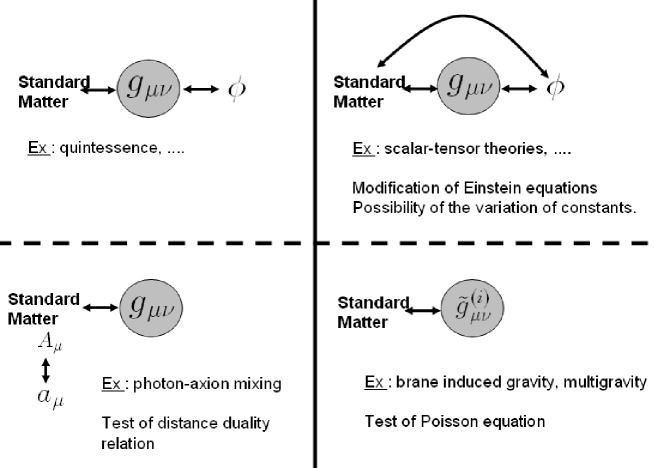
Figure 1: Summary of the different classes of models and of the specific tests that can help distinguish between them (besides the equation of state and the growth of cosmic structures). The classes differ according to the kind of new fields and to the way they couple to the metric $g_{\mu\nu}$ and to the standard matter fields. Upper-left class consists of models in which a new kind of gravitating matter is introduced, e.g. quintessence, K-essence. In the upper-right class, a light field induces a long-range force so that gravity is not described by a spin-2 graviton only. This is the case of scalar-tensor theories of gravity. In this class, Einstein equations are modified and there may be a variation of the fundamental constants. Note also the possibility for this new field to couple differently to baryonic and dark matter. The lower-right class corresponds to models in which there may exist massive gravitons, such as in some class of braneworld scenarios. These models predict a modification of the Poisson equation on large scales. In the last class (lower-left), the distance duality relation may be violated. From Ref. [24].

2.2 What is tested and what should we test?

Up to now, the observational status concerning the tests of gravity is the following.

1. On Solar System size, the Newton law as well as the universality of free fall are tested with a very good accuracy (see Ref. [5] for a summary of the constraints) .

2. On galactic scales, there are a number of astrophysical constraints that a successful modification of gravity will have to face (see e.g. Ref. [26]). If the modification of gravity has some relevance on galactic scales then it will have to explain the flattening of the rotation curves and to account for the dependence of the galaxy rotation curve on the luminosity of the galaxy. This dependence is encapsulated in the Tully-Fischer relation relating the luminosity of a spiral galaxy to its asymptotic rotation velocity $L\propto v_{\infty}^{\alpha}$, with $\alpha\sim 4$. This sets severe constraints on theories in which the cross-over scale with standard gravity is fixed (see e.g. Ref [27]) and favored theories where this cross-over scale depends on the considered galaxy. Roughly, one needs this crossover scale to behave as

   $$\ell_{*}\simeq\sqrt{\ell_{0}GM}/c$$ (2)

   where $\ell_{0}\sim 10^{27}$m. On the other hand, the compatibility between X-ray and strong lensing observations tends to show that the Poisson equation holds up to roughly 2 Mpc [28].

3. On cosmological scales, there is at the moment no direct tests of gravity. Indeed the growth of cosmological structure can put some constraints but usually the observations entangle the properties of the matter and gravity. Both the acceleration of the universe and the variation of the constants (if confirmed) may be indications of the break-down of general relativity in this regime.

What should we test then? General relativity is based on Einstein equivalence principle that includes three hypothesis: (i) local Lorentz invariance, (ii) local position invariance and (iii) universality of free fall. If these hypothesis are valid, it is thought that gravity is a geometric property of spacetime (see e.g. Ref. [29]). We may thus aim to test for both the Einstein equivalence principle and the field equations that determine the geometric structure created by any mass distribution. Some tests in these directions have been proposed in the past years.

• Lorentz invariance: it can be tested through the propagation of high energy particles. A summary of the constraints can be found in e.g. Ref. [30]

• Poisson equation: on sub-Hubble scales, the Einstein equations in an expanding spacetime reduce to the Poisson equation

  $$\Delta\Phi=4\pi G\rho a^{2}\delta$$ (3)

  that relates the gravitational potential to the density contrast. It was recently argued [31] that the comparison of galaxy catalogs such as SDSS or 2dF and of weak lensing observations give a direct test of this equation and can be extended up to 100 Mpc (see also Ref. [32]).

• Distance duality: as long as photons travel on null geodesics and the geodesic deviation equation holds, it can be shown that there is a reciprocity relation, $r_{S}=r_{O}(1+z)$ between the source and observer area distances. Indeed $r_{S}$ cannot be measured so that this relation cannot be tested. However, if the number of photons is conserved, it translates to a distance duality relation between the luminosity and angular distances, $D_{L}=D_{A}(1+z)^{2}$ that can be tested. This proposition [33] has been tested [24] using X-ray and Sunayev-Zeld’ovich observations of galaxy clusters and no departure from the standard expectation has been found (see Fig. 2). This can constrain e.g. models involving photon-axion mixing [34].

• Growth of cosmic structures: the growth factor of cosmic structures is sensitive to the equation of state of the matter that drives the expansion of the universe [35]. It was recently proposed to use the skewness and higher moments of the density field induced during the non-linear Newtonian clustering to test for the existence of a long-range Yukawa force [36]. Similarly, it was argued that this skewness was sensitive to the coupling of dark energy to dark matter [37, 38].

• Testing for the constancy of the (non-gravitational) constants is a direct test of the local invariance position that makes it a test of Einstein equivalence principle and of the strong equivalence principle when the gravitational constant is considered. It has been investigated by many methods and is the subject of the following section. Note that if violated, one expects also a violation of the universality of free fall mainly because the self-energy is composition dependent and gravitates.

Figure 2: $\eta={D_{A}}/{D_{L}}(1+z)^{2}$ as a function of the redshift for the 18 clusters of the Reese et al. [40] catalog. The error bars include the observational error bars as determined by Reese et al. [40] and the uncertainties in the cosmological parameters. Outlayers correspond to bimodal clusters that cannot be well fitted by a $\beta$-profile. This shows that there is no significant departure from the expected distance duality relation. From Ref. [24].

Figure 3: In a theory in which gravity switches from a standard four dimensional gravity to a five dimensional gravity above a crossover scale of $r_{s}=50h^{-1}$ Mpc, there are different cosmological implications concerning the growth of cosmological perturbations. Since gravity becomes weaker on large scales, fluctuations stop growing [left panel]. It implies [right panel] that the density contrast power spectrum (thick line) differs from the standard one (thin line) but, more important, from the gravitational potential power spectrum (dash line). From Ref. [31].

3 Update on the constraints on the variation of the constants

Since the claim [41] that the fine structure constant, $\alpha$, may have been smaller in the past, there have been a tremendous increase in the interest of the fundamental constants of nature and to whether there are really constant. Various reviews [3, 42] exist and details and more references can be found in Ref. [3]

We review the recent developments concerning mainly the constraints on the variation of the fine structure constant, as well as the proton to electron mass ration, $\mu$, and the gravitational constant, $G$.

3.1 Laboratory constraints

There have been some marked improvements on the constraints on the variation of $\alpha$ in laboratory experiments. These methods are based on the comparison of atomic clocks using different types of transitions in different atoms. According to the comparison, one can constrain the variation of some combination of fundamental constants. For instance, the hyperfine transition frequency of alkali can be approximated by [43]

$$\nu\propto\alpha^{2}\frac{\mu}{\mu_{N}}\frac{m_{\rm e}}{m_{\rm p}}R_{\infty}cF_{\rm rel}(Z\alpha)$$ (4)

where $\mu$ is the magnetic moment of the nucleus, $\mu_{N}$ the nuclear magneton, $R_{\infty}$ the Rydberg constant and $F_{\rm rel}$ a relativistic function [43] which strongly increases with the atom number $Z$ (e.g. ${\rm d}\ln F_{\rm rel}(Z\alpha)/{\rm d}\ln\alpha\simeq 0.74$ for ¹³³Cs and 0.30 for ⁸⁷Rb).

The comparison of hyperfine transitions in ⁸⁷Rb and ¹³³Cs over a period of about 4 years took advantage of this sharp variation to show [44] that ${\rm d}\ln(\nu_{\rm Rb}/\nu_{\rm Cs})/{\rm d}t=(0.2\pm 7.0)\times 10^{-16}\,{\rm yr}^{-1}$ at 1$\sigma$. Neglecting possible changes in the amplitude of the weak and strong interactions and thus in the nuclear magnetic moments, it translates to

$$\dot{\alpha}/\alpha=(-0.4\pm 16)\times 10^{-16}\,{\rm yr}^{-1}.$$ (5)

Another experiment [45] comparing an electric quadrupole transition in ¹⁹⁹Hg⁺ to the ground-state hyperfine splitting of ¹³³Cs over a 3 years period showed that $|{\rm d}\ln(\nu_{\rm Hg}/\nu_{\rm Cs})/{\rm d}t|<7.0\times 10^{-15}\,{\rm yr}^{-1}$. This constrains the time variation of $g_{\rm Cs}(m_{\rm e}/m_{\rm p})\alpha^{6.0}$ so that

$$\left|\dot{\alpha}/\alpha\right|<1.2\times 10^{-15}\,{\rm yr}^{-1}$$ (6)

if both the gyromagnetic factor $g_{\rm Cs}$ and $m_{\rm e}/m_{\rm p}$ are assumed constant.

The comparison [46] of the absolute $1S-2S$ transition in atomic hydrogen to the ground state of cesium combined with the results of Refs. [44, 45] yields the two independent constraints

$$\dot{\alpha}/\alpha=(-0.9\pm 2.9)\times 10^{-16}\,{\rm yr}^{-1},\qquad{\rm d}\ln(\nu_{\rm Rb}/\nu_{\rm Cs})/{\rm d}t=(-0.5\pm 1.7)\times 10^{-15}\,{\rm yr}^{-1}.$$ (7)

The comparison [47] of optical transitions in ¹⁷¹Yb⁺ to a cesium atomic clock at two times separated by 2.8 years has shown that ${\rm d}\ln(\nu_{\rm Yb}/\nu_{\rm Cs})/{\rm d}t=(-1.2\pm 4.4)\times 10^{-15}\,{\rm yr}^{-1}$ which translates to

$$\dot{\alpha}/\alpha=(-0.3\pm 2.0)\times 10^{-15}\,{\rm yr}^{-1}.$$ (8)

These methods allow to set very sharp local constraints and, as illustrated by the results of Ref. [46], they can be combined to set independent constraints on various constants.

3.2 Geochemical constraints

Sharp constraints on the time variation of the fine structure constant can be also obtained from the Oklo phenomenon and from the study of the lifetimes of long-lived nuclei.

The Oklo phenomenon is a natural nuclear reactor that operated during 200,000 years approximatively two billion years ago, that is at a redshift $z\sim 0.14$. The isotopic abundances of the yields give access to informations about the nuclear rates at that time. One of the key quantity measured is the ratio ${}^{149}_{62}{\rm Sm}/{}^{147}_{62}{\rm Sm}$ of two light isotopes of samarium which are not fission products. This ratio of order of 0.9 in normal samarium, is about 0.02 in Oklo ores. This low value is interpreted by the depletion of ${}^{149}_{62}{\rm Sm}$ by thermal neutrons to which it was exposed while the reactor was active. The capture cross section of thermal neutron by ${}^{149}{\rm Sm}$

$${}^{149}{\rm Sm}+n\rightarrow^{150}{\rm Sm}+\gamma$$ (9)

has a resonant energy $E_{r}\simeq 0.0973$ eV, which is a consequence of a near cancellation between electromagnetic and strong interactions [48]. A detailed analysis and model of the samarium nuclei lead [49], assuming that the variation of $E_{r}$ is due only to the $\alpha$ dependence of the electromagnetic energy, to the constraint

$$\Delta\alpha/\alpha=(0.15\pm 1.05)\times 10^{-7}$$ (10)

at 2$\sigma$. In particular, the accuracy of the method can be understood by comparing the resonant energy $E_{r}\sim 0.1$ eV to its sensitivity to a variation of $\alpha$, ${\rm d}E_{r}/{\rm d}\ln\alpha\sim-1$ Mev so that variation smaller than $\Delta\alpha/\alpha\sim 0.1\,{\rm eV}/1\,{\rm MeV}\sim 10^{-7}$ are expected.

It was later pointed out [50] that there may be two ranges of solutions compatible with the Oklo data

$$\Delta\alpha/\alpha=(-0.8\pm 1.0)\times 10^{-8},\qquad\Delta\alpha/\alpha=(8.8\pm 0.7)\times 10^{-8},$$ (11)

the second branches being disfavored by the analysis of the isotopic ratio of gadolinium.

Recently, the assumption that the low energy neutron spectrum is well described by a Maxwell-Boltzmann distribution was investigated [51]. The effect of a variation of the strange quark mass was studied [52] to show that $m_{\rm s}/\Lambda_{\rm QCD}$ has varied by less than $1.2\times 10^{-10}$ while assuming all fundamental couplings to vary independently led [53] to the more stringent limit $\Delta\alpha/\alpha<(1-5)\times 10^{-10}$.

Radioactive decay lifetimes can also be used once the $\alpha$-dependence of the decay rate is known. For instance, the lifetime of a $\beta$- decay nuclei scales as

$$\lambda\sim\Lambda(\Delta E)^{p}G_{F}^{2}\alpha^{s}$$ (12)

where $\Delta E$ is the decay energy and $s$ the sensitivity. Many nuclei were used but the sharpest constraint was obtained from the $\beta$-decay of rhenium to osmium by electron emission

$${}^{187}_{75}{\rm Re}\longrightarrow{}^{187}_{76}{\rm Os}+\bar{\nu}_{e}+e^{-},$$ (13)

first considered by Peebles and Dicke [54]. Interestingly, due its low decay energy –about 2.5 keV– the sensitivity of rhenium is $s\sim-18,000$ so that a variation of $\alpha$ of order $10^{-2}\%$ induces a variation decay energy of order of the keV.

The analysis of new meteorite and laboratory led to [55]

$$\Delta\alpha/\alpha=(8\pm 16)\times 10^{-7}$$ (14)

over the last 4.5 Gyr, which corresponds to $z\simeq 0.45$.

There is a caveat to this method that is not so direct: the ratio Re/Os is measured in iron meteorite the age of which is not determined directly. Models of formation of the solar system tend to show that iron meteorites and angrite meteorites form within the same 5 million years. The age of the latter can be estimated from the ²⁰⁷Pb-²⁰⁶Pb method which gives 4.558 billion years. Besides, this constraint holds on the averaged value of $\alpha$ over the 4.5 past billion years.

3.3 Cosmological constraints

On cosmological scales, the observation of the cosmic microwave background (CMB) anisotropies and of the abundances of the light elements produced during the big-bang nucleosynthesis (BBN) allow to set constraints of order $10^{-2}$ on the variation of $\alpha$.

Changing the fine structure constant modifies the strength of the electromagnetic interaction and thus its only effect on CMB anisotropies arises from the change in the differential optical depth of photons due to the Thomson scattering, $\dot{\tau}=x_{\rm e}n_{\rm e}c\sigma_{\rm T}$, which enters in the collision term of the Boltzmann equation describing the evolution of the photon distribution function and where $x_{\rm e}$ is the ionization fraction (i.e. the number density of free electrons with respect to their total number density $n_{\rm e}$). The first dependence of the optical depth on the fine structure constant arises from the Thomson scattering cross-section given by $\sigma_{\rm T}=({8\pi}/{3})({\hbar^{2}}/{m_{\rm e}^{2}c^{2}})\alpha^{2}$. The second, and more subtle dependence, comes from the ionization fraction. A variation of the fine structure constant can thus be thought of as considering a delayed recombination model.

Early works [56, 58, 57] based on BOOMERanG and MAXIMA data tend to show that the fit to CMB data are improved by allowing $\Delta\alpha\not=0$ while Landau et al. [59] concluded from these data imply, assuming spatially flat models with adiabatic primordial fluctuations, that $-0.14<\Delta\alpha/\alpha<0.03$ at $2\sigma$ level. The recent analysis [60] of the WMAP data (see the contribution by G. Rocha for details) gave the

$$\Delta\alpha/\alpha=(-1.5\pm 3.5)\times 10^{-2}$$ (15)

at $z\sim 10^{3}$. Note that he variation of the gravitational constant can also have similar effects on the CMB [61]. In conclusion, constraints of order $1\%$ on the variation of $\alpha$ can be obtained from the CMB only if the cosmological parameters are independently known.

BBN theory predicts the production of the light elements in the early universe the abundances of which rely on a fine balance between the expansion of the universe and the weak interaction rates which controls the neutron to proton ratio at the onset of BBN. Basically, the abundance of helium-4 is given by

$$Y_{p}=2\frac{(n/p)_{\rm f}\exp(-t_{\rm N}/\tau)}{1+(n/p)_{\rm f}\exp(-t_{\rm N}/\tau)}$$ (16)

where $(n/p)_{\rm f}=\exp{(-Q/kT_{f})}$ is the neutron to proton ratio at the freeze-out time determined by $G_{F}^{2}(kT_{\rm f})^{5}=\sqrt{GN}(kT_{\rm f})^{2}$, $N$ being the number of relativistic degrees of freedom; $Q=m_{\rm n}-m_{\rm p}$, $\tau$ is the neutron lifetime, $G_{F}$ the Fermi constant and $t_{\rm N}$ the time after which the photon density becomes low enough for the photo-dissociation to be negligible. As a conclusion, the predictions of BBN involve a large number of fundamental constants.

A change in $\alpha$ affects directly $Q$ and was modelled [62, 63] as $Q/\Lambda_{\rm QCD}=a\alpha+bv/\Lambda_{\rm QCD}$ where $v$ determines the weak scale and $a$ and $b$ are two numbers. Roughly, this implies that $\Delta Y/Y\sim-\Delta Q/Q\sim 0.6\Delta\alpha/\alpha$. On this basis, one can set the constraint $|\Delta\alpha/\alpha|<5\times 10^{-2}$ [62, 63], confirmed by a recent analysis [64] which gives $|\Delta\alpha/\alpha|<6\times 10^{-2}$. This does not take the effect of the fine structure constant in the Coulomb barriers and in the cross-sections, which was investigated in Ref. [65]. Recently, the effect of seven parameters $(G,\alpha,v,m_{e},\tau,Q,B_{d})$, later related to the six constants $(G,\alpha,v,m_{e},m_{u},m_{d})$ was taken into account and led to the constraint [66]

$$\Delta\alpha/\alpha=(6\pm 4)\times 10^{-4}.$$ (17)

The effect of the strange quark mass was also investigated [52] and it was claimed that $m_{\rm s}/\Lambda_{\rm QCD}$ has varied by less than $6\times 10^{-3}$ since BBN.

3.4 Astrophysical constraints

Most of the excitement over the possibility of the fine structure constant variation arises from the observation of distant quasar absorption systems. The method is based on the comparison of absorption spectra to laboratory spectra.

Initially, the method was based on alkali doublets, the splitting of which gives access to the fine structure constant, $\Delta\nu/\bar{\nu}\propto\alpha^{2}$. The analysis of Si IV on 21 systems gave [69] $\Delta\alpha/\alpha=(-0.5\pm 1.3)\times 10^{-5}$ for $2\leq z\leq 3$. The most recent constraint [70] has been obtained from the analysis of SiIV in 15 systems of the VLT/UVES sample, improving the former constraint by a factor 3,

$$\Delta\alpha/\alpha=(0.15\pm 0.43)\times 10^{-5},\qquad 1.59\leq z\leq 2.92.$$ (18)

It is to be noted that none of the analysis based on the alkali doublet method exhibit a hint of variation of $\alpha$.

The many multiplet (MM) method proposed by Webb et al. [41, 68] was aimed at increasing the precision of the AD method by correlating several transition lines from various species in order to reach a sensitivity of order $10^{-6}$. In particular, one can compare line shifts of element which are sensitive to variation in $\alpha$ with those that are not. At low redshift ($z\leq 1.8$), the results lie mainly on the comparison of Fe to Mg while at higher redshift they lie on the comparison of Fe and Si. The latest analysis [67] of the Keck/Hires data (see Fig. 4) based on 128 systems in the range $0.5\leq z\leq 3$ points toward a lower value of $\alpha$ in the past

$$\Delta\alpha/\alpha=(-0.54\pm 0.12)\times 10^{-5},\qquad 0.5\leq z\leq 3$$ (19)

as previous analysis did [41, 68]. A detailed budget of the errors was done and a possible systematic effects was looked at but none was exhibited. Note also that new synthetic atomic spectra were produced [71].

Recent observations from the VLT/UVES using the same MM method have not been able to duplicate this result [72, 73] (see Fig. 4). The analysis by Chand et al. [72] is mainly based on the analysis of Fe and Mg in 23 systems toward 18 QSOs in the range $0.4\leq z\leq 2.3$ because they apply some selection criteria to the lines. In particular (1) they kept only species with similar ionization potentials (MgII, FeII, SiII and AlII) so that they are most likely to originate from similar regions in the cloud, (2) absorption lines that are contaminated by atmospheric lines were rejected, (3) they put a threshold on the column density so that all FeII multiplets are detected at 5$\sigma$, (4) they checked that the anchor are not saturated (Mg I and II are fairly insensitive to variation of $\alpha$) and (5) they excluded strongly saturated systems with large velocity spread. They concluded [72, 73] that

$$\Delta\alpha/\alpha=(-0.6\pm 0.6)\times 10^{-6},\qquad 0.4\leq z\leq 2.3$$ (20)

at 1$\sigma$. The analysis of a single quasar [74] also gave

$$\Delta\alpha/\alpha=(-0.1\pm 1.7)\times 10^{-6},\qquad z=1.15$$ (21)

mainly from the analysis of Fe lines. These results were further confirmed by the analysis of Fe II lines in an absorption system at $z=1.839$ toward the quasar Q1101-264 [75]

$$\Delta\alpha/\alpha=(2.4\pm 3.8)\times 10^{-6},\qquad z=1.839.$$ (22)

The combined Fe II sample also gives $\Delta\alpha/\alpha=(0.4\pm 1.5)\times 10^{-6}$ for two systems at $z=1.15$ and $1.839$.

Both results [67, 72] are sensitive to the isotopic abundances of magnesium and assume a solar ratio ²⁴Mg:²⁵Mg:²⁶Mg=79:10:11. It is however commonly assumed that heavy magnesium isotopes are absent in low metallicity environments such as absorption clouds. Assuming a ratio 1:0:0 would have led to a more significant detection of $\Delta\alpha/\alpha=(-0.98\pm 0.13)\times 10^{-5}$ and $\Delta\alpha/\alpha=(-0.36\pm 0.06)\times 10^{-5}$ respectively for the Keck/Hires [67] and VLT/UVES [72] data. This has led to a new interpretation [76] of the MM results in which the variation of $\alpha$ is explained by an early nucleosynthesis of ²⁵Mg and ²⁶Mg. Interestingly a ratio [72] (²⁵Mg+²⁶Mg)/²⁴Mg = $0.62\pm 0.05$ and $0.30\pm 0.01$ can explain respectively the Keck/Hires [67] and VLT/UVES [72] data. A model of nucleosynthesis in which ²⁵Mg and ²⁶Mg are produced by intermediate mass ($4-6M_{\odot}$) in their asymptotic giant branch was proposed. They can reach a temperature larger than $7\times 10^{7}$K so that proton capture processes in the Mg-Al cycle are effective enough. This hypothesis can be tested by looking at other heavy elements produced by these intermediate mass stars.

To finish, let us mention the use of O III emission lines of quasars and galaxies. The analysis [77] of 42 quasars from SDSS early data release and of 165 quasars of SDSS data release 1 led respectively to the two constraints

$$\Delta\alpha/\alpha=(0.7\pm 1.4)\times 10^{-4},\qquad\Delta\alpha/\alpha=(1.2\pm 0.7)\times 10^{-4}$$ (23)

in the range $0.16\leq z\leq 0.8$. The use of the OH microwave transition was also proposed [78] and the preliminary analysis of the quasar PKS1412+135 led to [79]

$$\Delta\alpha/\alpha=(0.51\pm 1.26)\times 10^{-4},\qquad z=0.2467.$$ (24)

These methods can be extended to higher redshifts ($z\sim 3-5$) and have different systematics compared to the MM and AD methods which makes them complementary. Also, the analysis of OH, combined with HCO⁺ lines gave the simultaneous bounds [80] $\Delta\alpha/\alpha=(-0.38\pm 2.2)\times 10^{-3}$, $\Delta\mu/\mu=(-0.27\pm 1.6)\times 10^{-3}$ and $\Delta g_{p}/g_{p}=(-0.77\pm 4.2)\times 10^{-3}$ at z=0.68.

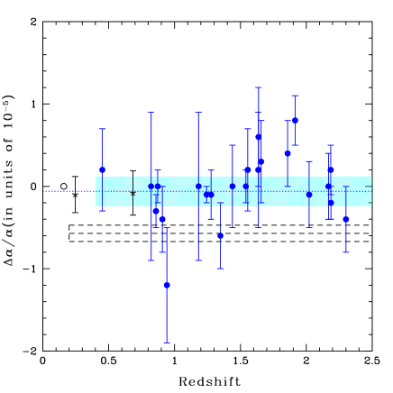
Figure 4: The analysis of quasar spectra on the variation of the fine structure constant from (left) the Keck/Hires data [67] and (right) the VLT/UVES data [72]. The left plot depicts their previous low redshift (open circles), previous high redshift (open triangles) and new (open squares) samples. The raw results with $1\sigma$ error bar are shown on the top panel while the middle panel shows the results with an arbitrary bining and the bottom panel combines the three samples. The right plot present the results from the VLT/UVES data [72]. The dash lines represent the weighted mean and $1\sigma$ range from the analysis of Ref. [67] while the dash region marks the weighted mean and its $3\sigma$ error bars.

3.5 Other constants

3.5.1 Proton to electron mass ratio

The observation of vibro-rotational transitions of H₂ in damped Lyman-$\alpha$ systems allows to constrain the variation of the proton to electron mass ratio, $\mu=m_{\rm p}/m_{\rm e}$. The spectral lines of the quasar are usually translated into a reduced redshift, defined as $\zeta_{i}\equiv(z_{i}-\bar{z})/(1+\bar{z})$ where $\bar{z}$ is the averaged redshift of the absorption system. It can be shown that $\zeta_{i}=({\Delta\mu}/{\mu})K_{i}$ where the $K_{i}$ are sensitivity coefficients.

Various constraints have been obtained since 1975 all showing no hint of variation. In particular, the analysis of 83 absorption lines [81] gave the limit

$$\Delta\mu/\mu=(-7.5\pm 9.5)\times 10^{-5}$$ (25)

at a $2\sigma$ level. More recently, the analysis of vibro-rotational lines of molecular hydrogen for the two quasars Q1232+082 ($z=2.3377$) and Q0347-382 ($z=3.0249$) tend to show [82] that

$$\Delta\mu/\mu=(-5.7\pm 3.8)\times 10^{-5}$$ (26)

at $1.5\sigma$. It has recently been revised [84] to

$$\Delta\mu/\mu=(2.97\pm 0.74)\times 10^{-5}.$$ (27)

It was shown that the limiting factor of the analysis was the precision of the determination of the spectra in the laboratory. New data for the transition wavelengths of H₂ Lyman and Werner bands have been obtained with an accuracy of $5\times 10^{-8}$ [83]. The reanalysis of the published spectra then led to $\Delta\mu/\mu=(-0.5\pm 3.0)\times 10^{-5}$ at $2\sigma$ level, confirming, once again, that the determination of the laboratory spectra is the key of the debate on a possible variation of $\mu$.

3.5.2 Gravitational constant

Few new works concern the gravitational constant. Let us note a new analysis of the BBN [85] that tends to show that

$$\Delta G/G=0.01^{+0.20}_{-0.16}$$ (28)

at 68% C.L. It was also shown [64] that the variation of $G$ is correlated to the extra-number of relativistic degrees of freedom through $\Delta G/G=7\delta N/43$. It follows that the combined analysis of new ⁴He and WMAP data implies

$$-0.10<\Delta G/G<0.13$$ (29)

A recent analysis of the secular variation of the period of nonradial pulsations of the white dwarf G117-B15A shows [86] that $0<\dot{G}/G<4.0\times 10^{-11}\,{\rm yr}^{-1}$ at 2$\sigma$, which is of the same order of magnitude of previous independent bounds (see also Ref. [87]).

More important, in the Solar System, the measurement of the frequency shift of radio photon to and from the Cassini spacecraft improved the constraint on the post-Newtonian parameter $\gamma$ to [88] $\gamma-1=(2.1\pm 2.3)\times 10^{-5}$. This can be translated, in a model dependent way, into a constraint on the time variation of $G$. For instance in a Brans-Dicke theory in a matter dominated universe, it implies $|\dot{G}/G|\leq 10^{-14}\,\mathrm{yr}^{-1}$.

4 Theoretical motivations and modelling

4.1 From string theory to phenomenology

Most higher dimensional theories, such as Kaluza-Klein and string theories, imply that dimensionless constants are dynamical [25, 89]. For example, in type I superstring, the 10-dimensional dilaton couples differently to the gravitational and Yang-Mills sectors because the graviton is an excitation of closed strings while the Yang-Mills fields are excitations of open strings. For small value of the volume of the extra-dimensions, a T-duality makes the theory equivalent to a 10-dimensional theory with Yang-Mills fields localized on a D3 brane. When compactified on an orbifold, the gauge fields couple to fields $M_{i}$ living only at these orbifold points with coupling $c_{i}$ which are not universal. Typically, one gets that $M_{4}^{2}=\hbox{e}^{-2\Phi}V_{6}M_{I}^{8}$ while $g_{YM}^{-2}=\hbox{e}^{-2\Phi}V_{6}M_{I}^{6}+c_{i}M_{i}$. Loop corrections have also been studied in heterotic theory by including Kaluza-Klein excitations [90]. In the limit where the volume is large compared to the mass scale, $g_{YM}^{-2}=\hbox{e}^{-2\Phi}V_{6}M_{H}^{6}-b_{a}(RM_{H})^{2}/2+\ldots$. Again, they are not universal. It follows that the 4-dimensional effective couplings depend on the version of the string theory, on the compactification scheme and on the dilaton.

Interestingly, while the constraints presented above assume that only $\alpha$ was varying, it is to be expected that if it varies then all other constants also do. In the context of unified theories, it is possible to derive relations between the variations of various constants, which can be used to derive sharper observational constraints. The dominant effects [97] arise from the variation of the QCD scale, $\Lambda_{\rm QCD}$ and the weak scales $v$. In particular it was argued [91, 92] that $\Delta\Lambda_{\rm QCD}/\Lambda_{\rm QCD}\sim 30\Delta\alpha/\alpha$ and $\Delta v/v\sim 80\Delta\alpha/\alpha$.

Many phenomenological models starting from the investigation by Bekenstein [93] have been developed [94, 95] as well as some braneworld models with varying constant were constructed [96]. Damour and Polyakov [97] proposed to capture the features of loop corrections by modelling them as a genus expansion, that is as a series in the string coupling constant. The low energy action involves various couplings of the effective four-dimensional dilaton to the different matter fields. It follows that generically there appear couplings to matter fields via their Yang-Mills couplings and masses as as a potential for the scalar field. This construction includes others such as the Bekenstein model [93]. Note that these models are required in order to compare constraints at various time.

This phenomenology is related to the one of quintessence and the light field responsible for the time variation of the constants may also be the cosmon [18]. In that sense, the variation of the constant may shed some light on the physics on dark energy. Initially models of scalar-tensor quintessence [16, 17] were considered. Some were using the Damour-Nordtvedt attraction mechanism toward general relativity to pass the Solar System constraints. The Damour-Polyakov model [97] was generalized [98] to a runaway potential so that the light dilaton accounts for the variation of the constants, the acceleration of the universe and is at the origin of a violation of the universality of free fall.

4.2 Two Dangers

The construction of phenomenological models that tend to explain the small drift of the constant in the late universe by introducing a slow-rolling scalar field have two dangers to avoid.

First, such a light field will obey a Klein-Gordon like equation, $\ddot{\phi}+3H\dot{\phi}=-m^{2}\phi+\ldots$. In order for this field not to oscillate but still be evolving, its mass needs to be very small, typically $m\sim H_{0}\sim 10^{-33}$ eV. The question arises of the mechanism that protects it from radiative corrections, a problem common with most quintessence models. Various solutions have been proposed among which the possibility for this field to be a pseudo-Goldstone boson [99] or to identify this light field with shape modulus [100].

A second danger lies in the violation of the universality of free fall due to the composition dependence of the self energy and of the masses. This was illustrated in Bekenstein original construction [93] and was further studied with linear [102] and quadratic [101] couplings. In the case of a light dilaton, it was shown that if it were to remain massless then it would induce a violation of the universality of free fall seven order of magnitudes larger than the actual bounds [97]. To avoid such a catastrophe, it has either to suddenly take a mass larger than a few meV (so that gravity will be compatible with Einstein gravity above a millimeter) or decouple from matter [97]. This latter mechanism is analogous to the original Damour-Nordtvedt attraction mechanism [103]. Both mechanisms have different implications concerning the variation of the coupling constants. A fixed point [104] or the recently proposed chameleon mechanism [105] also claimed to bypass this problem. A consequence is that the improvement of the tests of the universality of free fall by 2 or 3 orders of magnitude may give some surprises.

4.3 Varying constants in the early universe

Inflation universally produces classical almost scale free Gaussian inhomogeneities of any light scalars. Assuming the coupling constants at the time of inflation depend on some light moduli fields, it was shown [106] that modulated cosmological fluctuations are produced during (p)reheating. This idea was extended to hybrid inflation [107] where the bifurcation value of the inflaton is modulated by the spatial inhomogeneities of the couplings. As a result, the symmetry breaking after inflation occurs not simultaneously in space but with the time laps in different Hubble patches inherited from the long-wavelength moduli inhomogeneities. In this model, the consistency relation of inflation is modified. These light field can also be at the origin of non-Gaussianity [108].

If couplings depend on the value of some light fields, then they have most probably developed super-Hubble correlations of typical amplitude $10^{-5}$, simply because the quantum fluctuations of any light field are amplified during inflation. It follows that one expects spatial variation with these correlation (see e.g. Ref. [98]). They may have some observational effects [109], in particular on the CMB [110] polarization and Gaussianity.

5 Conclusions

In conclusion, testing for the variation of fundamental constants is a test of fundamental physics, and in particular of general relativity. It completes other tests that can be applied on cosmological scales. Such tests are needed to substantiate the physics of the dark sector that plays an increasing role in cosmology.

While observational constraints become sharper, the debate on $\alpha$ is not over yet but recent observations have not been able to reproduce the detection of a lower $\alpha$ in the past [41, 68, 67]. More important, there now exists a physical model, requiring no new physics, to interpret the supposed variation of $\alpha$ as an enhancement of heavy isotopes of magnesium. We can now hope that the debate will be settled in the coming years.

The future will offer new constraints, particularly with atomic clocks in space (ACES), new tests of the universality of free fall (recent launch of $\mu$SCOPE) as well as new methods, as illustrated by the recent activity. These developments will probably shed some light on a possible scalar field acting in the late universe or on some new structures such as higher dimensions.

Acknowledgments I thank G. Esposito-Farèse, E. Flam, P. Petitjean and C. Schimd for many discussions on this subject, as well as my collaborators in some of the works presented here, N. Aghanim, F. Bernardeau and Y. Mellier. I am grateful to the organizers of the workshop for their kind invitation.

References

- [1] P.A.M. Dirac, Nature (London) 139, 323 (1937); Proc. Roy. Soc. London A 165, 198 (1938).
- [2] P. Jordan, Naturwiss. 25, 513 (1937); Z. Physik 113, 660 (1939).
- [3] J.-P. Uzan, Rev. Mod. Phys. 75 (2003) 403.
- [4] R.H. Dicke, in Relativity, Groups and Topology, Lectures delivered at Les Houches 1963, ed. by C. DeWitt and B. DeWitt, (Gordon and Breach, New York, 1964).
- [5] C.D. Hoyle et al., [arXiv:hep-ph/0405262].
- [6] J. P. Uzan, Annales Henri Poincare 4 (2003) S347; ibid., Int. J. Theor. Phys. 42 (2003) 1163.
- [7] M. Fukugita and P.J.E. Peebles, [arXiv:astro-ph/0406095].
- [8] G. F. R. Ellis and J.- P. Uzan, [arXiv:gr-qc/0305099].
- [9] L. Okun, Sov. Phys. Usp. 34 (1991) 818.
- [10] M. Duff, L. Okun, G. Veneziano, JHEP 0203 (2002) 023.
- [11] R. Lehoucq and J.P. Uzan, Les constantes fondamentales (Belin, Paris, 2005).
- [12] B. Ratra and P.J.E. Peebles, Rev. Mod. Phys. 75 (2003) 559.
- [13] C. Wetterich, Nucl. Phys. B 302 (1988) 668; B. Ratra and P.J.E. Peebles, Phys. Rev. D 37 (1988) 3406; I. Zlatev, L. Wand and P. Steinhardt, Phys. Rev. Lett. 82 (1999) 896.
- [14] C. Armendariz-Picon, V. Mukhanov, and P.J. Steinhardt, Phys. Rev. D64 (2001) 103510; T. Chiba, T. Okabe, and M. Yamagushi, Phys. Rev. D62 (2000) 023511.
- [15] S.M. Carroll, Living Rev. Rel. 4 (2001) 1; V. Sahni and A. Starobinski, Int. J. Mod. Phys. D 9 (2000) 373.
- [16] J. P. Uzan, Phys. Rev. D 59, 123510 (1999).
- [17] T. Chiba, Phys. Rev. D 60 (1999) 083508; L. Amendola, Phys. Rev. D62 (2000) 043511.
- [18] C. Wetterich, [arXiv:hep-ph/0301261].
- [19] R. Gregory, V.A. Rubakov, and S.M. Sibiryakov, Phys. Rev. Lett. 84, 4690 (2000).
- [20] I.I. Kogan, et al., Nucl. Phys. B 584, 313 (2000).
- [21] G. Dvali, G. Gabadadze, and M. Porati, Phys. Lett. B 485, 208 (2000); V. Sahni and Y. Shtanov, JCAP 0311 (2003) 014.
-
[22]
B. Carter, et al.,
Class. Quant. Grav. 18, 4871 (2001);
J. P. Uzan,
Int. J. Theor. Phys. 41 (2002) 2299;
J. P. Uzan, Int. J. Mod. Phys. A 17 (2002) 2739. - [23] G.F.R. Ellis and M. Madsen, Class. Quant. Grav. 8 (1991) 667.
- [24] J. P. Uzan, N. Aghanim, and Y. Mellier, [arXiv:astro-ph/0405620].
- [25] T.R. Taylor, and G. Veneziano, Phys. Lett. B 213, 450 (1988); E. Witten, Phys. Lett. B 149, 351 (1984).
- [26] A. Aguirre, et al., Class. Quant. Grav. 18, R223 (2001).
- [27] R.H. Sanders, Month. Not. R. Acad. Soc. 223, 539 (1986).
- [28] S. W. Allen et al., Mon. Not. Roy. Astron. Soc. 324, 842 (2001).
- [29] C. M. Will, Living Rev. Relativity 4 (2001) 4.
- [30] T. Jacobson, S. Liberati and D. Mattingly, [arXiv:gr-qc/0404067].
- [31] J. P. Uzan and F. Bernardeau, Phys. Rev. D 64, 083004 (2001).
- [32] M. J. White and C. S. Kochanek, Astrophys. J. 560 (2001) 539.
- [33] B. A. Bassett and M. Kunz, Phys. Rev. D 69 (2004) 101305; ibid, Phys. Rev. D 69 101305 (2004).
- [34] C. Csaki, N. Kaloper, and J. Terning, Phys. Rev. Lett. 88 (2002) 161302; C. Deffayet et al., Phys. Rev. D 66 (2002) 043517.
- [35] K. Benabed and F. Bernardeau, Phys. Rev. D 64 (2001) 083501.
- [36] C. Sealfon, L. Verde and R. Jimenez, [arXiv:astro-ph/0404111].
- [37] L. Amendola and C. Quercellini, Phys. Rev. Lett. 92 (2004) 181102.
- [38] R. R. Reis, M. Makler and I. Waga, Phys. Rev. D 69 (2004) 101301.
- [39] G.F.R. Ellis, Q. Jl. R. astr. Soc. 16 (1975) 245. [arXiv:astro-ph/0407003].
- [40] E.D. Reese et al., Astrophys. J. 581 (2002) 53.
- [41] J. Webb et al., Phys. Rev. Lett. 82 (1999) 884.
- [42] T. Damour, Astrophys. Space Sci. 283 (2003) 445; T. Damour, [arXiv:gr-qc/0306023].
- [43] S.G. Karshenboim, [arXiv:physics/0311080].
- [44] H. Marion et al., Phys. Rev. Lett. 90 (2003) 150801.
- [45] S. Bize et al., Phys. Rev. Lett. 90 (2003) 150802.
- [46] M. Fischer et al., Phys. Rev. Lett. 92 (2004) 230802.
- [47] E. Peik et al., [arXiv:physics/0402132].
- [48] A.I. Shlyakhter, Nature (London) 264 (1976) 340.
- [49] T. Damour and F. Dyson, Nucl. Phys. B 480 (1996) 37.
- [50] Y. Fujii et al., Nucl. Phys. B 573 (2000) 377.
- [51] S.K. Lamoreaux and J.R. Torgerson, Phys. Rev. D 69 (004) 121701.
- [52] V.V. Flambaum and E.V. Shuryak, Phys. Rev. D 67 (2002) 083507.
- [53] K. Olive et al., Phys. Rev. D 66 (2002) 045022.
- [54] P.J.E. Peebles and R. Dicke, Phys. Rev. 128 (1962) 2006.
- [55] K. Olive et al., Phys. Rev. D 69 (2000) 027701.
- [56] P.P. Avelino et al., Phys. Rev. D 62, 123508 (2000).
- [57] P.P. Avelino et al., Phys. Rev. D 64, 103505 (2001).
- [58] R.A. Battye, R. Crittenden, and J. Weller, Phys. Rev. D 63, 0453505 (2001).
- [59] S. Landau, D.D. Harari, and M. Zaldarriaga, Phys. Rev. D 63, 083505 (2001).
- [60] C. Martins et al., Phys. Lett. B 585 (2004) 29; G. Rocha et al., N. Astron. Rev. 47 (2003) 863.
- [61] A. Riazuelo and J.- P. Uzan, Phys. Rev. D 66, 023525 (2002).
- [62] B.A Campbell, and K.A. Olive, Phys. Lett. B 345 (1995) 429.
- [63] E.W. Kolb, M.J. Perry, and T.P. Walker, Phys. Rev. D 33 (1996) 869.
- [64] R.H. Cyburt et al., [arXiv:astro-ph/0408033].
- [65] L. Bergström, S. Iguri, and H. Rubinstein, Phys. Rev. D 60 (1999) 045005.
- [66] C.M. Müller, G. Sachäfer, and C. Weterich, [arXiv:astro-ph/0405373].
- [67] M.T. Murphy et al., Month. Not. R. Astron. Soc. 345 (2003) 609.
- [68] J. Webb et al., Phys. Rev. Lett. 87 (2001) 091301.
- [69] M.T. Murphy et al., Month. Not. R. Astron. Soc. 327 (2003) 1237.
- [70] H. Chand et al., [arXiv:astro-ph/0408200].
- [71] J.C. Berengut et al., [arXiv:physics/0408017].
- [72] H. Chand et al., Astron. Astrophys. 417 (2004) 853.
- [73] R. Srianand et al., Phys. Rev. Lett. 92 (2004) 121302.
- [74] R. Quast et al., Astron. Astrophys. 415 (2004) L7.
- [75] S.A. Levshakov et al., [arXiv:astro-ph/0408188].
- [76] T. Ashenfelter et al., Phys. Rev. Lett. 92 (2004) 041102.
- [77] J. Bahcall, , C.L. Steinhardt, and D. Schlegel, Astrophys. J. 600 (2004) 520.
- [78] J. Darling, Phys. Rev. Lett. 91 (2003) 011301.
- [79] J. Darling, [arXiv:astro-ph/0405240].
- [80] J. Chengalur and N. Kanekar, Phys. Rev. Lett. 91 (2003) 241303; N. Kanekar and J. Chengalur, MNRAS 350 (2004) L17.
- [81] A.Y. Potekhin et al., Astrophys. J. 505 (1998) 523.
- [82] A. Ivanchik et al., Astrophys. Space Sci. 283 (2003) 583.
- [83] W. Ubachs and E. Reinhold, Phys. Rev. Lett. 92 (2004) 101302.
- [84] P. Petitjean et al., C. R. Acad. Sci. (Paris) 5 (2004) 411.
- [85] C.J. Copi, A.N. Davis, and L.M. Krauss, Phys. Rev. Lett. 92 (2004) 171301.
- [86] O.G. Benvenuto, E. Garcia-Berro, and J. Isern, Phys. Rev. D 69 (2004) 082002.
- [87] M. Biesada and B. Malec, Month. Not. R. Astron. Soc. 350 (2004) 644.
- [88] B. Bertotti, L. Iess, and P. Tortora, Nature (London) 425 (2003) 374.
- [89] J. Polchinski, Superstring theory (Cambridge University Press, 1997).
- [90] E. Dudas, Class. Quant. Grav. 17 (2000) R41.
- [91] X. Calmet and H. Fritzsch; Eur. J. Phys. C24 (2002), 639; ibid, [hep-ph/0204258].
- [92] T. Dent and M. Fairbairn, 2001, Nuc. Phys. B 653 (2003) 256.
- [93] J.D. Bekenstein, Phys. Rev. D 25 (1982) 1527.
- [94] C. Armendáriz-Picón, Phys. Rev. D 66 (2002) 064008.
- [95] K. Olive and M. Pospelov, Phys. Rev. D 65 (2002) 085044.
- [96] G.A. Palma, et al.. [arXiv:astro-ph/0306279].
- [97] T. Damour, and A.M. Polyakov, Nuc. Phys. B 423 (1994) 532.
- [98] T. Damour, F. Piazza and G. Veneziano, Phys. Rev. D 66 (2002) 046007; ibid, Phys. Rev. Lett. 89 (2002) 081601.
- [99] S. Carroll, Phys. Rev. Lett. 81 (2001) 3067.
- [100] M. Peloso and E. Poppitz, Phys. Rev. D68 (2003) 125009.
- [101] S. Lee, K. Olive, and M. Pospelov, [arXiv:astro-ph/0406039].
- [102] P.P. Avelino et al., [arXiv:astro-ph/0402379].
- [103] T. Damour and K. Nordtvedt, Phys. Rev. Lett. 70 (1993) 2217.
- [104] C. Wetterich, [arXiv:hep-th/0210156].
- [105] J. Khouri and A. Veltman, [arXiv:astro-ph/0309300].
- [106] L. Kofman, [arXiv:astro-ph/0303614] ; G. Dvali, A. Gruzinov and M. Zaldarriaga, [arXiv:astro-ph/0303591].
- [107] F. Bernardeau, L. Kofman, and J. P. Uzan, [arXiv:astro-ph/0403315].
- [108] F. Bernardeau and J.-P. Uzan, Phys. Rev. D 66 (2002) 103506; Phys. Rev. D 67 (2003) 121301(R); [arXiv:astro-ph/0311421].
- [109] D. Mota and J. Barrow, Month. Not. R. Astron. Soc. 349 (2004) 281.
- [110] K. Sigurdson et al., Phys. Rev. D 68 (2003) 103509.