Is Dark Energy Dynamical? Prospects for an Answer

Abstract

Recent data advances offer the exciting prospect of a first look at whether dark energy has a dynamical equation of state or not. While formally theories exist with a constant equation of state, they are nongeneric – Einstein’s cosmological constant is a notable exception. So limits on the time variation, $w^{\prime}$, directly tell us crucial physics. Two recent improvements in supernova data from the Hubble Space Telescope allow important steps forward in constraining the dynamics of dark energy, possessing the ability to exclude models with $w^{\prime}\mathrel{\mathchoice{\lower 3.6pt\vbox{\halign{$\mathsurround=0pt\displaystyle\hfil#\hfil$\cr>\crcr\sim\crcr}}}{\lower 3.6pt\vbox{\halign{$\mathsurround=0pt\textstyle\hfil#\hfil$\cr>\crcr\sim\crcr}}}{\lower 3.6pt\vbox{\halign{$\mathsurround=0pt\scriptstyle\hfil#\hfil$\cr>\crcr\sim\crcr}}}{\lower 3.6pt\vbox{\halign{$\mathsurround=0pt\scriptscriptstyle\hfil#\hfil$\cr>\crcr\sim\crcr}}}}1$, if the universe truly has a cosmological constant. These data bring us much closer to the “systematics” era, where further improvements will come predominantly from more accurate, not merely more, observations. We examine the possible gains and point out the complementary roles of space and ground based observations in the near future. To achieve the leap to precision understanding of dark energy in the next generation will require specially designed space based measurements; we estimate the confidence level of detection of dynamics (e.g. distinguishing between $w^{\prime}=0$ and $w^{\prime}=1$) will be $\sim 1.8\sigma$ after the ongoing generation, improving to more than $6.5\sigma$ in the dedicated space generation.

I Introduction

The acceleration of the expansion of the universe represents a critical mystery. To the physicist this raises questions about Einstein’s general relativity, quantum physics, and extra dimensions. To the interested spectator it contains the determination of the fate of the universe.

We will not learn a unique answer to all these questions without an overall theory for the dark energy causing the acceleration – one possibility for which is Einstein’s cosmological constant. But a major question that is directly accessible is whether the dark energy is dynamical, possessing a variation in time, sufficient in itself to rule out a cosmological constant. Observations of the expansion, most clearly and directly at present through the use of Type Ia supernovae as calibrated candles for the distance-redshift behavior, can constrain the physics through the measured properties of the dark energy.

These properties are conveniently described by the equation of state ratio of dark energy pressure to density, determining how the dark energy evolves with cosmic time $t$ or redshift $z$, and written $w(z)$. Generically there is such an evolution, though the cosmological constant possesses an unchanging $w=-1$. It is difficult to estimate a typical value for the rate of change without a fundamental theory. But let’s make what appears to be a reasonable assumption that the dark energy behavior responds to the cosmic expansion $a(t)$, so the equation of state changes on a timescale related to the transition from matter domination to dark energy domination, or slower due to the influence of the remaining matter. Then a variation less than or of the same order of the Hubble expansion rate $H=\dot{a}/a$ seems natural:

$$\dot{w} \equiv \frac{dw}{dt}=H\frac{dw}{d\ln a}\lesssim H,$$ (1)

$$w^{\prime} \equiv \frac{dw}{d\ln a}\lesssim 1.$$ (2)

We caution that our notions of naturalness do not constrain the universe to actually act that way!

In §II we examine what the quality of the most recent supernovae data can tell us about the magnitude of $w^{\prime}$. We emphasize that this is an illustrative look, based on estimated types of data numbers and accuracy, rather than the actual data themselves. Possible future samples involving more data and better data are examined in §III to see how they give the greatest leverage on improving our knowledge of the dynamic nature of dark energy. We conclude in §IV with thoughts on what new advances are required to understand the fate of our universe.

II Data and Dynamics

For constraining the nature of dark energy, we consider three forms of data currently available. Type Ia supernovae (SN) magnitudes and redshifts play a central role in tracing the expansion history of the universe, and led to the discovery of the acceleration perl99 ; riess98 . When expanding the description of dark energy to include not only the contribution of its energy density but its present equation of state $w_{0}$ and a measure of its time variation $w^{\prime}$, other types of data are crucial to break the degeneracies between the parameters. So we also consider cosmic microwave background (CMB) measurements of the distance to the last scattering surface, and a prior on the matter density $\Omega_{m}$ from large scale structure surveys. The role of CMB complementarity with SN measurements was emphasized in fhlt .

II.1 Method

Our parameter set includes ${\cal M}$ – a “nuisance” parameter combining the supernova absolute magnitude and the Hubble constant – and the matter density $\Omega_{m}$, present dark energy equation of state $w_{0}$, and time variation $w^{\prime}$. We assume a flat universe, which current CMB data are consistent with but future measurements will further refine. As our fiducial cosmology we adopt $\Omega_{m}=0.28$ and a cosmological constant. For the CMB prior we take the WMAP determination of the reduced distance to last scattering measured with a 3.3% relative precision. Similarly, a gaussian prior of 0.03 on $\Omega_{m}$ is used. The major role of the priors is to break degeneracies between parameters rather than determine $w^{\prime}$ per se. Neither of these priors is fully descriptive of the complementary probe data, but are adequate approximations for the level of precision desired for the estimation of $w_{0}$ and $w^{\prime}$.

The time variation $w^{\prime}$ is taken from the form for the dark energy equation of state

$$w(z)=w_{0}+w_{a}(1-a),$$ (3)

where the scale factor $a=(1+z)^{-1}$, so $w^{\prime}=w_{a}/2$ when evaluated at $z=1$. (This value is what we mean by $w^{\prime}$ for the rest of the paper.) This parametrization is very successful in modeling a great variety of dark energy (and extended gravity) models linprl ; lingrav and $z=1$ is a natural epoch to measure a characteristic time variation. At higher redshifts, in the matter dominated era, dark energy is often very slowly varying, while at later times many models approach the cosmological constant value of $w=-1$. This parametrization allows high redshift data from supernovae and the CMB to be combined easily with lower redshift data, since $w(z)$ is bounded and well behaved. Note that the parametrization $w(z)=w_{0}+w_{1}z$, which is unbounded at high redshifts, is unphysical for the CMB data, and a poor approximation for SN data at $z>1$.

For sufficiently large positive $w_{a}$ the asymptotic value of the dark energy equation of state at high redshift $w(z\gg 1)=w_{0}+w_{a}$ will become positive. This would break matter domination and cause problems with, e.g. structure formation, and so these models are disfavored. This could be either physically true or an indication that the parametrization incorporates the CMB prior poorly. This ambiguity is not a problem if the data constrain $w_{a}\mathrel{\mathchoice{\lower 3.6pt\vbox{\halign{$\mathsurround=0pt\displaystyle\hfil#\hfil$\cr<\crcr\sim\crcr}}}{\lower 3.6pt\vbox{\halign{$\mathsurround=0pt\textstyle\hfil#\hfil$\cr<\crcr\sim\crcr}}}{\lower 3.6pt\vbox{\halign{$\mathsurround=0pt\scriptstyle\hfil#\hfil$\cr<\crcr\sim\crcr}}}{\lower 3.6pt\vbox{\halign{$\mathsurround=0pt\scriptscriptstyle\hfil#\hfil$\cr<\crcr\sim\crcr}}}}1$. We find that in weak data cases the Monte Carlo estimations of the parameter uncertainties stray into a small region of phase space with $w(z\gg 1)>0$, making the estimate of the positive (plus) error on $w^{\prime}$ unreliable. In those cases we will give the parabolic uncertainty (local estimation assuming a quadratic shape around the minimum) and the negative (minus) error (see discussion below regarding robustness of the majority of the Monte Carlo contour). Despite these slight flaws in the parametrization when dealing with weak data constraints, the affected regions of parameter space are much smaller than in the $w_{1}$ case, which is more severely pathological and runs into trouble even for the SN sample.

Our fiducial, illustrative supernova sample comprises 40 local SN, placed in a bin centered at $z=0.05$, and 10 medium redshift SN per bins of redshift width 0.1 centered at $z=0.15$, 0.25,…0.85. This gives 120 SN. We supplement this with a high redshift sample of 1 per bin for $z=0.95-1.65$. Again, we emphasize this does not represent an actual data set, just a broad description of the types of data recently available. We examine in §3 the consequences of increasing the numbers of SN in each of the three subsamples.

Because we expect errors in $w_{0}$ and $w_{a}$ to be large, a Fisher method of analysis may not guarantee accurate estimations. We employ both Fisher and Monte Carlo simulations to obtain our results; Fisher methods allow rapid exploration of changes in the supernova numbers and systematic errors, providing a guide to interesting areas that are then confirmed through Monte Carlo analysis.

Statistical uncertainties of 0.15 magnitudes, including intrinsic dispersion and measurement errors, are placed on each SN and then a systematic floor $dm$ is placed on the error in each redshift bin. The two types of errors are added in quadrature and the errors are assumed uncorrelated from bin to bin. So for $N$ SN in a bin, the total magnitude error per bin is

$$dm_{\rm tot}=\sqrt{dm^{2}+0.15^{2}/N}.$$ (4)

We will see that the systematic uncertainties play a key role. As a fiducial model we take the magnitude systematic to be $dm=A_{0}+Az$. Including the presence of systematics at low redshift, $A_{0}\neq 0$, is a crucial element since this has a strong effect on ${\cal M}$ and, through its correlations, on the other parameters. This model is clearly a cartoon representation of a very complex error propagation problem, but it is tractable and should give a not unreasonable estimation klmm . We emphasize that we do not claim the systematics model represents any current or planned experiment. No missions were harmed during the writing of this paper.

Because of the excitement of a first estimate of the time variation $w^{\prime}$, we concentrate on this parameter, marginalizing over the others, quoting both the negative and parabolic (or positive, where available) estimation uncertainties; see the figures for the Monte Carlo contours. For certain cases we present as well the limits that would be produced on $w_{0}$ or a constant $w$ (with $w^{\prime}$ forced to zero).

II.2 Previous data

First consider the low and medium redshift SN only. Without priors, and taking $dm=0.03+0.07z$, we cannot reasonably determine $w^{\prime}$ simultaneously with the other parameters. Upon inclusion of the CMB and $\Omega_{m}$ priors, we obtain a negative estimation uncertainty of $\sigma_{\_}(w^{\prime})=1.46$ (1.14 parabolic). Note that if $A=0.12$ instead of 0.07 then the limit is 1.22 parabolic. There are few enough SN that the systematic floor does not have a big effect. So with such data we have not restricted $w^{\prime}$ more tightly than our “naturalness” argument of Eq. (2). Data leading to results improving on that ad hoc bound would be a welcome advance.

II.3 High redshift supernovae

Now let’s add the sample of high redshift ($z>0.9$) SN. For SN at $z>0.9$ we take $dm=0.1z$. Without external priors $w^{\prime}$ still cannot be determined; with the priors we find $\sigma_{\_}(w^{\prime})=1.05$ (0.90 parabolic) (from now on we always include the priors). For the higher systematics case, $dm=0.03+0.12z$ for $z<0.9$ and $dm=0.15z$ for $z>0.9$, the parabolic errors jump to 1.01.

So the high redshift SN (with priors) begin to bring our knowledge below the naturalness bound – a useful step. But we will see that for further improvement we simultaneously need to understand low redshift supernovae as well, to keep the systematics small, as discussed in §III.

II.4 High accuracy supernovae

High redshift supernovae, keeping magnitude uncertainties within the systematic bounds considered, require observations from space. Currently the Hubble Space Telescope (HST) is the only such data source, and has demonstrated an exciting ability to discover and characterize small samples of high redshift SN riess04 .

Moreover HST has also contributed accurate observations of medium redshift SN that have proved excellent for constraining systematic uncertainties such as dust extinction knop . We examine the role that this type of data plays. To focus on this last aspect, in this subsection we do not include the high redshift SN (but do in §3).

If the systematics uncertainty is reduced to $dm=0.03+0.04z$ through such observations, then the constraint on $\sigma(w^{\prime})$ (with priors) becomes 1.08 parabolic. Such an improvement in systematics, without high redshift SN, provides roughly 1/4 of the improvement that adding the SN out to $z=1.65$, as in §II.3, would. Of course this progress is greater – roughly 2/3 as good an improvement – if the systematics in §II.3 were at the higher level considered. So high accuracy measurements are a valuable criterion in addition to high redshift measurements in our quest to understand the nature of dark energy.

III Future improvements

Both accuracy and redshift range play a critical role, we just saw. HST has enabled strong advances on these two fronts, with the existence of the riess04 and knop data, though again we do not view our models as representing any real data set. If both improvements are combined, using $dm=0.03+0.04z$ for $z<0.9$ and $dm=0.1z$ for $z>0.9$, the uncertainty $\sigma_{\_}(w^{\prime})$ improves slightly to 1.0 (0.87 parabolic). Understanding of low redshift SN, which functions both to limit systematics and essentially calibrate ${\cal M}$ (and hence reduce degeneracies with other parameters), is a goal of the Nearby Supernova Factory project now underway snf . We simulate this forthcoming information by taking $dm=0.01+0.06z$ for $z<0.9$. The numbers then become $\sigma_{\_}(w^{\prime})=0.89$ (0.77 parabolic), demonstrating the important roles of systematics control and low redshift SN. Note there is considerable asymmetry between the parabolic and negative (and hence positive) uncertainties. The uncertainty on the present equation of state $w_{0}$ is 0.30. If one forces $w^{\prime}=0$, then the constant equation of state is estimated within 0.12 (but gives very limited physical insight because of confusion in interpretation recon , since we don’t know a priori that $w^{\prime}=0$).

Several of the Monte Carlo contours discussed are plotted in Fig. 1. Asymmetry between the positive and negative excursions of the parameters is evident, even excluding from consideration the highly positive $w^{\prime}$ region containing a small part of the contour. We indicate the cut off in the upper left region where we should not believe results as they pile up near the $w(z\gg 1)\geq 0$ boundary. With improved data the contours will become wholly distinct from the problematic region (the best fit should lie elsewhere since our universe did form structure).

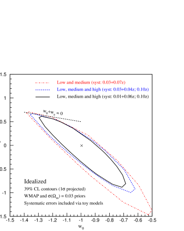
Figure 1: Contours show Monte Carlo estimations of the dark energy equation of state today, $w_{0}$, and a measure of its time variation, $w^{\prime}=w_{a}/2$, for various types of supernova data sets and systematic uncertainties. The contours enclose 39% of the probability so $1\sigma$ estimation of the parameters is found by projection to the respective axis. Contour points near the $w_{0}+w_{a}=w(z\gg 1)=0$ boundary line are not robust but the vast majority of the contour is valid.

III.1 Idealistic estimations

Can we look forward to rapid, further improvement in our knowledge beyond the leap made in the last year, through statistical gains as more supernovae are analyzed (other high redshift supernovae have already been found)?

Suppose we increase by a factor 10 the sample at low/medium/high redshift. We adopt the model $dm=0.01+0.06z$ for $z<0.9$, $dm=0.1z$ for $z>0.9$ from now on. The parabolic uncertainties in $w^{\prime}$ become 0.68/0.65/0.69 or approximately 10-15% improvements. The systematics floor severely limits any statistical improvement.

So while the most recent HST data has led to an appreciable gain in our knowledge, we cannot expect a further dramatic improvement through merely gathering more supernovae. The recent advances have brought us to the threshold of the systematics limited era of revealing dark energy. This is an important and sobering conclusion. Let’s investigate this further.

III.2 More realistic estimations

The comprehensive supernova programs over the next several years (e.g. essence ; snls ) may indeed allow a tenfold increase in the low and medium redshift samples, and we also consider a more challenging tenfold increase in the $z>0.9$ sample in addition. Before we quantify the effects of all these together, however, we recognize that when we approach higher precision in parameter estimation we need to take into account more seriously other systematics, which can again inflate the uncertainties.

For one thing, the heterogeneity of the data samples will both increase the dispersion and can lead to biased results. Joining together diverse SN data, taken with different instruments under different conditions can lead to a coherent systematic, basically a calibration offset. This can have a pernicious influence through biasing the cosmological parameter estimation (see the discussion in §4 of klmm , for example). While many samples may contribute to the tenfold increase in SN data, we assume sufficient uniformity that we only worry about an offset between local and medium redshift SN, and medium and high redshift. One can view these as arising either from greatly differing telescopes, e.g. wide field, small aperture vs. smaller field, larger aperture vs. space based, or from different filter sets, e.g. including U, Z, I, J, etc. beyond the usual B, V bands. For a toy model we consider coherent magnitude offsets of 0.02 between the low and medium redshift samples and 0.04 between the medium and high samples. Biases from those offsets would amount to a nonnegligible $0.5-1\sigma$ shift in the cosmological parameter estimations. While serious, this effect is not included in our quoted $\sigma(w^{\prime})$ precisions in the remainder of this paper.

A variation is to consider the case where the possibility of such a systematic is recognized, and such offsets are incorporated as fitting parameters. As a toy model we allow new parameters describing these magnitude shifts to float subject to gaussian constraints of 0.02 (low-medium redshift samples) and 0.04 (medium-high) magnitudes. In this case the cosmology will not be biased from the true model but the parameter estimations will suffer increased dispersion. Allowing for a 10 times sample increase for low, medium, and high SN (corresponding to 400 SN at $z<0.1$, 100/bin for $z=0.1-0.9$, and 10/bin for $z=0.9-1.7$, for a total of 1280 SN) and incorporating this calibration systematic yields an uncertainty of $\sigma(w^{\prime})=0.58$. (Now the contours are small enough to be wholly valid: the positive error is +0.52, the negative is -0.64, and their mean agrees with the parabolic error of 0.58).

An experiment that spectrophotometrically ties the local and medium redshift SN and creates a homogeneous sample over the entire range $z=0.1-1.7$, necessarily space based, removes both versions of this systematic problem and is required for tighter constraints.

A second major systematic involves the current dominant source of systematics uncertainty: correction for dust extinction. This uncertainty may well grow as we include SN appearing in higher redshift galaxies. For example, the value of the coefficient in the dust reddening law, $R_{V}$, may change or possess increased scatter, which in turn affects the corrected peak magnitude. (See, for example, mortsellgoobar .) Here we again neglect the coherent effect which may cause bias (see discussion in the conclusion section) and concentrate on the incoherent scatter.

The toy model here takes a magnitude systematic of 0.02 or 0.05, correlated within a redshift bin but uncorrelated from bin to bin. This can be viewed as an uncertainty on $R_{V}$ of 0.2 (or 0.5) with a color excess parameter fixed at $E(B-V)=0.1$. These numbers seem reasonable as, for example, rv finds that $R_{V}$ can easily be different from the fiducial 3.1 by $\pm 0.5$. The presence of such a systematic degrades the estimation of $w^{\prime}$ for the tenfold increased sample (1280 SN) by 19% (63%) for 0.02 (0.05) mag scatter. The effect on $w_{0}$ is even more pronounced, at 31% (106%).

Again, a survey that tightly characterizes the SN photometry over multiple wavelengths bands from the blue to the near infrared, hence space based, strongly constrains the wavelength dependence of the reddening, i.e. $R_{V}$, and this source of error.

Treating the calibration and extinction systematics as the two main uncertainties, we can address within our toy models what is the most “optimistically realistic” prospect before the next generation of experiments for determining whether dark energy is dynamical. We view this optimistically as coming from a set of 1280 SN (though as shown this is already systematics saturated so more SN will not change the conclusions) covering the range $z=0-1.7$ with a calibration systematic as discussed above and an extinction systematic at the lower, 0.02 mag value. Our baseline prediction then is that $\sigma(w^{\prime})=0.68$ (as well the uncertainty on $w_{0}$ is 0.28 and for a forced constant $w$ is 0.11). If one were less optimistic and used 0.05 mag for the extinction systematic then $\sigma(w^{\prime})=0.90$. Since Planck CMB data should be available on about the same time scale as the tenfold increase in the SN sample, we note that using Planck data instead of WMAP brings $\sigma(w^{\prime})$ to 0.57 (0.79 with 0.05 mag extinction systematic), though still $\sigma(w_{0})=0.27$.

Figure 2 illustrates the parameter estimations given the vastly enlarged data sets, but also taking into account the two systematic effects of heterogeneity of data sets and uncertain extinction corrections. As always, we caution these are merely illustrative, toy models. The tenfold increase in the $z>0.9$ sample provides little of the improvement, because of the systematics wall – pointing up the crucial role of systematics reduction. Our most optimistic near term prospect of $\sigma(w^{\prime})=0.57$ represents a possible limit below the “naturalness bound” of $1.75\sigma$ (if the data are best fit by $w^{\prime}=0$).

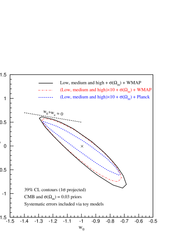
Figure 2: As Fig. 1, for various types of data sets that might become feasible through future experiments. The solid black curve is the same as in Fig. 1; other curves take 10 times the statistics but include two further sources of systematics: data sample heterogeneity and extinction correction scatter.

To distinguish the various dark energy theories common in the literature, however, to obtain practical knowledge of the nature of dark energy, will require a further generation of SN experiment, with tight systematics control over the entire redshift range from 0.1-1.7, say. In particular, we emphasize the vital significance of the improvements that would be obtained. For example, a derived value of $w^{\prime}=0\pm 0.57$ gives a less than $2\sigma$ favoring of the cosmological constant below the naturalness bound – scarcely sufficient for a problem of such critical implications. A next generation space based experiment dedicated to systematics control could realistically attain (in combination with Planck) $\sigma(w^{\prime})<0.15$ (cf. omni ). This would provide a “separation power” of $w^{\prime}=0$ from $w^{\prime}=1$ at $6.7\sigma$ significance, far more robust and worthwhile for such fundamental physics. Naïvely, in these terms the prospect without a next generation corresponds to having a $\sim 10$% “unconfidence” level in whether dark energy is dynamical, while the next generation could reduce this to $10^{-11}$ – quite a leap forward.

Finally, we emphasize that this has been only an illustrative look at the prospects of exploring the dynamic nature of dark energy. The quantitative results here are dependent on the very simple characterization of the SN distribution, priors, and especially systematic uncertainties, and should not be taken as more than a broad indication of trends.

IV Conclusion

A great step in our knowledge of dark energy involves the characterization of its dynamical properties, i.e. the value of the time variation in its equation of state. The first step is whether it is consistent with a cosmological constant possessing no variation, i.e. limited below a “naturalness” bound $w^{\prime}\lesssim 1$. Measurements of supernovae with the Hubble Space Telescope can achieve this reduction, by extending the reach of the magnitude-redshift data to higher redshifts and by increasing the accuracy of the characterization of the supernovae. Such data should provide limits roughly around $\sigma(w^{\prime})\approx 0.8-0.9$.

Such a step forward brings us near to a systematics wall, however, at least at high redshifts, diminishing the prospects for further improvements by strengthened statistics. The generation of surveys just beginning, however, will provide more data to learn about supernovae, blending valuable measurements at low and high redshifts, from both ground and space based instruments. By identifying and constraining systematic uncertainties they pave the way for the next, space based generation to obtain tight, physically revelatory bounds on the dark energy dynamics. As well, improvements will come in the external priors.

We caution that systematic uncertainties play a major role in translating the observations to knowledge of the nature of dark energy. One example is gravitational lensing: the true magnitude of any single SN at some redshift is strongly uncertain since gravitational lensing by structure in the universe imposes a divergent variance on the magnitude; averaging over several SN is required to bring the highly nongaussian dispersion down to near the intrinsic SN magnitude dispersion (holzlinder , also see §7 of klmm , and amanullah ).

Another caution is apparent from Figure 13 of knop . Systematic uncertainties that act to dim the supernovae, such as dust extinction, tend to drive the derived equation of state $w(z)$ more negative. If not fully accounted for, the data may indicate a more strongly negative $w(z)$, for example a $w^{\prime}<0$, than for the true nature of the dark energy. (Conversely, overcorrection can lead to $w^{\prime}>0$). The coherent extinction systematic mentioned in §III.2 in fact can bias a true cosmological constant to appear as a strongly $w_{0}<-1$, $w^{\prime}>0$ (or $w_{0}>-1$, $w^{\prime}<0$) model. Further investigation of a variety of biases is a subject of future work.

Models with $w^{\prime}<0$ do exist, such as the linear potential model, and can lead to future collapse as discussed in the “cosmic doomsday” scenario of kallosh . Whether $w^{\prime}>0$ or $w^{\prime}<0$ thus has profound future impact, so to learn whether the fate of our universe is collapse or eternal expansion first requires stringent control of systematics. The dramatic step beyond the $w^{\prime}$ bounds of the next few years will come from space, from missions dedicated to systematics control. Quality not quantity is the watchword. We emphasize that an improvement from $\mathrel{\mathchoice{\lower 3.6pt\vbox{\halign{$\mathsurround=0pt\displaystyle\hfil#\hfil$\cr<\crcr\sim\crcr}}}{\lower 3.6pt\vbox{\halign{$\mathsurround=0pt\textstyle\hfil#\hfil$\cr<\crcr\sim\crcr}}}{\lower 3.6pt\vbox{\halign{$\mathsurround=0pt\scriptstyle\hfil#\hfil$\cr<\crcr\sim\crcr}}}{\lower 3.6pt\vbox{\halign{$\mathsurround=0pt\scriptscriptstyle\hfil#\hfil$\cr<\crcr\sim\crcr}}}}2\sigma$ to $\mathrel{\mathchoice{\lower 3.6pt\vbox{\halign{$\mathsurround=0pt\displaystyle\hfil#\hfil$\cr>\crcr\sim\crcr}}}{\lower 3.6pt\vbox{\halign{$\mathsurround=0pt\textstyle\hfil#\hfil$\cr>\crcr\sim\crcr}}}{\lower 3.6pt\vbox{\halign{$\mathsurround=0pt\scriptstyle\hfil#\hfil$\cr>\crcr\sim\crcr}}}{\lower 3.6pt\vbox{\halign{$\mathsurround=0pt\scriptscriptstyle\hfil#\hfil$\cr>\crcr\sim\crcr}}}}6\sigma$ detection of dynamics, or its lack, is a truly dramatic advance, and crucial to our understanding.

In addressing the question of whether dark energy is dynamic, we have moved from ignorance to possessing the capabilities to limit the more extravagant possibilities, and in the third generation begin precision distinction of the nature of dark energy. This will bring us much closer to knowledge of fundamental physics and the fate of the universe, whether deSitter expansion under the cosmological constant, superacceleration and a Big Rip under phantom energy (but see lingrav for an opposing conjecture about fate under superacceleration), or collapse under “cosmic doomsday” scenarios.

References

- (1) S. Perlmutter et al., Ap. J. 517, 565 (1999)
- (2) A. Riess et al., Astron. J. 116, 1009 (1998)
- (3) J.A. Frieman, D. Huterer, E.V. Linder, and M.S. Turner, Phys. Rev. D 67, 083505 (2003) [astro-ph/0208100]
- (4) E.V. Linder, Phys. Rev. Lett. 90, 091301 (2003) [astro-ph/0208512]
- (5) E.V. Linder, Phys. Rev. D 70, 023511 (2004) [astro-ph/0402503]
- (6) A.G. Kim, E.V. Linder, R. Miquel, and N. Mostek, MNRAS 347, 909 (2004) [astro-ph/0304509]
- (7) A.G. Riess et al., Ap. J. 607, 665 (2004) [astro-ph/0402512]
- (8) R.A. Knop et al., Ap. J. 598, 102 (2003) [astro-ph/0309368]
-
(9)
W.M. Wood-Vasey et al., New Astron. Rev. 48, 637 (2004)
[astro-ph/0401513];
http://snfactory.lbl.gov - (10) E.V. Linder, Phys. Rev. D 70, 061302 (2004) [astro-ph/0406189]
- (11) Essence Project: http://www.ctio.noao.edu/~wsne
- (12) SuperNova Legacy Survey: http://www.cfht.hawaii.edu/SNLS
- (13) E. Mörtsell and A. Goobar, JCAP 0309, 9 (2003) [astro-ph/0308046]
- (14) B.T. Draine, ARAA 41, 241 (2003) [astro-ph/0304489]
- (15) G. Aldering et al., astro-ph/0405232
- (16) D.E. Holz and E.V. Linder, in draft
- (17) R. Amanullah, E. Mörtsell, and A. Goobar, A&A 397, 819 (2003) [astro-ph/0204280]
- (18) R. Kallosh, J. Kratochvil, A. Linde, E.V. Linder, and M. Shmakova, JCAP 0310, 15 (2003) [astro-ph/0307185]