Particle decay during inflation:
self-decay of inflaton quantum fluctuations during slow roll.

Abstract

Particle decay during inflation is studied by implementing a dynamical renormalization group resummation combined with a small $\Delta$ expansion. $\Delta$ measures the deviation from the scale invariant power spectrum and regulates the infrared. In slow roll inflation, $\Delta$ is a simple function of the slow roll parameters $\epsilon_{V},\;\eta_{V}$. We find that quantum fluctuations can self-decay as a consequence of the inflationary expansion through processes which are forbidden in Minkowski space-time. We compute the self-decay of the inflaton quantum fluctuations during slow roll inflation. For wavelengths deep inside the Hubble radius the decay is enhanced by the emission of ultrasoft collinear quanta, i.e. bremsstrahlung radiation of superhorizon quanta which becomes the leading decay channel for physical wavelengths $H\ll k_{ph}(\eta)\ll H/(\eta_{V}-\epsilon_{V})$. The decay of short wavelength fluctuations hastens as the physical wave vector approaches the horizon. Superhorizon fluctuations decay with a power law $\eta^{\Gamma}$ in conformal time where in terms of the amplitude of curvature perturbations $\triangle^{2}_{\mathcal{R}}$, the scalar spectral index $n_{s}$, the tensor to scalar ratio $r$ and slow roll parameters :

$$\Gamma\simeq\frac{32\;\xi^{2}_{V}\;\triangle^{2}_{\mathcal{R}}}{(n_{s}-1+\frac{r}{4})^{2}}\left[1+\mathcal{O}(\epsilon_{V},\eta_{V})\right]\;.$$

The behavior of the growing mode ${\eta^{\eta_{V}-\epsilon_{V}+\Gamma}}/{\eta}$ features an anomalous scaling dimension $\Gamma$. We discuss the implications of these results for scalar and tensor perturbations as well as for non-gaussianities in the power spectrum. The recent WMAP data suggests $\Gamma\gtrsim 3.6\times 10^{-9}$.

I Introduction

A period of accelerated expansion in the early universe, namely inflation, is nowadays part of standard cosmology since explains the homogeneity, isotropy and flatness of the observed Universe guth -liddle . At the same time, inflation provides a mechanism for generating metric fluctuations which seed large scale structure: during inflation physical scales grow faster than the Hubble radius but slower than it during both radiation or matter domination eras, therefore physical wavelengths cross the horizon (Hubble radius) twice. Quantum fluctuations generated during inflation with wavelengths smaller than the Hubble radius become classical and are amplified upon first crossing the horizon. As they re-enter the horizon during the decelerated stage these fluctuations provide the seed for matter and radiation inhomogeneities which generate structure upon gravitational collapse mukhanov ; hawking ; guthpi ; starobinsky ; bardeen ; bran . Most of the inflationary models predict fairly generic features: a gaussian, nearly scale invariant spectrum of adiabatic scalar and tensor primordial perturbations (gravitational waves). These generic predictions are in spectacular agreement with Cosmic Microwave Background (CMB) observations. Gaussian komatsu and adiabatic nearly scale invariant primordial fluctuations spergel provide an excellent fit to the WMAP data as well as to a variety of large scale structure observations. Perhaps the most striking confirmation of inflation as the mechanism for generating superhorizon (‘acausal’) perturbations is the anticorrelation peak in the temperature-polarization (TE) angular power spectra at $l\sim 150$ corresponding to superhorizon scales kogut ; peiris . The anticorrelation between the E-mode (parity even) polarization fluctuation and the temperature fluctuation is a distinctive feature of superhorizon adiabatic fluctuations sperzalda : the (peculiar) velocity gradient generates a quadrupole temperature anisotropy field around electrons which in turn generates an E-polarization mode. By continuity, the gradient of the peculiar velocity field is related to the time derivative of the density (temperature) fluctuations, hence the peculiar velocity and the initial (adiabatic) contribution to the (acoustic) oscillations of the photon baryon fluid are out of phase by $\pi/2$ sperzalda . Thus, the product of these two terms gives an anticorrelation peak at $k\,c_{s}\;\eta_{dec}=3\,\pi/4$ which corresponds to superhorizon wavelengths since the size of the horizon is $\sqrt{3}$ larger than the size of the sound horizon. The WMAP (TE) data kogut ; peiris clearly displays the anticorrelation peak at $l\sim 150$ providing perhaps one of the most striking confirmations of adiabatic superhorizon fluctuations as predicted by inflation. While the robust predictions of a generic inflationary model seem to provide an excellent fit to the WMAP data, different models predict slight differences. Therefore, theoretical differences between different models as well as potential experimental deviations from the most generic features are the focus of intense study. With the ever increasing precision of CMB observations it is conceivable that forthcoming observations will allow a narrower determination of inflationary models. Relevant discriminants between models are: non-gaussianity, a running spectral index either for scalar and/or tensor perturbations, an isocurvature component of primordial fluctuations, etc. Already WMAP reports a hint of running spectral index of scalar perturbations from the blue on large scales to the red on small scales peiris . Quantum effects associated with interactions can potentially lead to non-gaussian correlationsallen -bartolo . Therefore the detection of a running index (as hinted in the WMAP data) or small non-gaussianities in the temperature correlations imply potentially interesting quantum phenomena during the inflationary stage that was imprinted on superhorizon scales.

The inflaton is usually studied as a homogeneous classical scalar fieldkolb ; coles ; liddle . However, important aspects of the dynamics require a full quantum treatment for their consistent description. The quantum dynamics of the inflaton is systematically treated within a non-perturbative framework and some consequences on the CMB anisotropy spectrum were analyzed in ref.cosmo .

In this article we study quantum phenomena during inflation which contribute to relevant observables in the CMB anisotropies and polarization. In particular, we focus on inflaton decay during inflation as a potential source of quantum phenomena contributing to deviations from scale invariance in the primordial power spectrum and/or to non-gaussian features. If the inflaton couples to other particles, then its quantum fluctuations which seed scalar density perturbations also couple to these other fields. Consequently, the decay of the amplitude of the quantum fluctuations of the inflaton may lead to a modification of the power spectrum of density perturbations. The same coupling that is responsible for the decay of the inflaton quantum fluctuations can be also the source of non-gaussian correlations.

Particle decay is a distinct feature of interacting quantum field theories and is necessarily an important part of the inflationary paradigm: the decay of the inflaton into lighter particles after inflation may yield to the radiation dominated stage. Recently, inflaton decay during a post-inflationary stage has been considered as a possible source of metric perturbations arising from an inhomogeneity in the inflaton coupling 7L . Inflaton decay has also been studied as a dissipative mechanism in the dynamics of the inflaton berera , however these studies only apply when the expansion rate is much smaller than the typical mass scales.

In a previous article desiterI we introduced and implemented a systematic program to study the relaxational dynamics and particle decay in the case of a rapidly expanding inflationary stage. Whereby rapid expansion refers to the Hubble parameter during inflation being much larger than the mass of the particles. In the case of the inflaton, this is the situation of relevance for slow-roll inflation and a necessary (although not sufficient) condition for an almost scale invariant power spectrum of scalar fluctuations linde ; kolb ; liddle ; lidsey . In ref.prem inflaton decay was studied in some particular cases for which a solution of the equations of motion was available. The method of ref.prem was recently applied to the study of the decay of the inflation in alternative de Sitter invariant vacuarich .

The Minkowski space-time computation of the decay rate is not suitable for a stage of rapid expansion (as quantified above): the rapid expansion of the Universe and the manifest lack of a global time-like Killing vector allow processes that would be forbidden by energy conservation in Minkowski space-time. As emphasized in woodard ; desiterI , the lack of energy conservation in a rapidly expanding cosmology requires a different approach to study particle decay. The correct decay law follows from the relaxation in time of the expectation value of the field out of equilibrium. The relaxation of the non-equilibrium expectation value of the field is computed in ref.desiterI using the dynamical renormalization group (DRG) which allows to extract the decay law directly from the real time equations of motion. The reliability and predictive power of the DRG has been tested for a wide range of physical situations including hot and dense plasmas in and out of equilibrium DRG .

The goals of this article: We compute the particle decay of quantum fields minimally coupled to gravity with masses $M$ much smaller than the Hubble parameter, which is the relevant case for slow roll inflation. This entails a much stronger infrared behavior than for massless particles conformally coupled to gravity. The emergence of infrared divergences in quantum processes with gravitons during de Sitter inflation has been the focus of a thorough study IRcosmo ; dolgov . As we will see in detail below, similar strong infrared behavior enters in the decay of minimally coupled particles with masses $M$ much smaller than the Hubble parameter $H$. When $M<<H$ there is a small parameter $\Delta\sim M^{2}/H^{2}$ which regulates the infrared behavior in de Sitter inflation. We find that a similar parameter $\Delta$ exists in quasi de Sitter slow roll inflation which is a simple function of the slow-roll parameters. $\Delta$ regulates the infrared in the self-energy corrections even for massless particles (gravitons).

We begin by studying the general case of a cubic interaction of scalar particles minimally coupled to gravity, allowing the decay of one field into two others during de Sitter inflation. The masses of all particles are much smaller than the Hubble constant, which leads to a strong infrared behavior in the self-energy loops. We introduce an expansion in terms of a small parameter $\Delta$ which regulates the infrared and which in the case of de Sitter inflation is determined by the ratio of the mass of the particle in the loop to the the Hubble constant. Long-time divergences associated with secular terms in the solutions of the equations of motion are systematically resummed by implementing the DRG introduced in refs.desiterI ; DRG and lead to the decay law. We then apply these general results to the case of quasi-de Sitter slow roll inflation. We show that in this case a similar small parameter $\Delta$ emerges which is a simple function of slow-roll parameters and regulates the infrared behavior even for massless particles. We study the decay of superhorizon fluctuations as well as of fluctuations with wavelengths deep inside the horizon. A rather striking aspect is that a particle can decay into itself precisely as a consequence of the lack of energy conservation in a rapidly expanding cosmology. We then focus on studying the decay of the inflaton quantum fluctuations into their own quanta, namely the self-decay of the inflaton fluctuations, discussing the potential implications on the power spectra of primordial perturbations and to non-gaussianity.

Brief summary of results:

• In the case of de Sitter inflation for particles with mass $M\ll H$ a small parameter $\Delta\sim M^{2}/H^{2}$ regulates the infrared. We introduce an expansion in this small parameter $\Delta$ akin to the $\varepsilon$ expansion in dimensionally regularized critical theories. We obtain the decay laws in a $\Delta$ expansion after implementing the DRG resummation.

• Minimally coupled particles decay faster than those conformally coupled to gravity due to the strong infrared behavior both for superhorizon modes as well as for modes with wavelengths well inside the Hubble radius.

• The decay of short wavelength modes, those inside the horizon during inflation, is enhanced by soft collinear bremsstrahlung radiation of superhorizon quanta which becomes the dominant decay channel when the physical wave vector obeys,

  $$k_{ph}(\eta)\lesssim\frac{H}{\eta_{V}-\epsilon_{V}}\;,$$ (1)

  where $\eta_{V},\epsilon_{V}$ are the standard potential slow roll parameters.

• An expanding cosmology allows processes that are forbidden in Minkowski space-time by energy conservationwoodard ; desiterI : in particular, for masses $\ll H$, kinematic thresholds are absent allowing a particle to decay into itself. Namely, the self-decay of quantum fluctuations is a feature of an interacting theory in a rapidly expanding cosmology. A self-coupling of the inflaton leads to the self-decay of its quantum fluctuations both for modes inside as well as outside the Hubble radius.

• The results obtained in de Sitter directly apply to the self decay of the quantum fluctuations of the inflaton during slow roll (quasi de Sitter) expansion. In this case, $\Delta$ is a simple function of the slow roll parameters. For superhorizon modes we find that the amplitude of the inflaton quantum fluctuations relaxes as a power law $\eta^{\Gamma}$ in conformal time. To lowest order in slow roll, we find $\Gamma$ completely determined by slow roll parameters and the amplitude of the power spectrum of curvature perturbations $\triangle^{2}_{\mathcal{R}}$:

  $$\Gamma=\frac{8\;\xi^{2}_{V}\;\triangle^{2}_{\mathcal{R}}}{(\epsilon_{V}-\eta_{V})^{2}}\left[1+\mathcal{O}(\epsilon_{V},\eta_{V})\right]$$ (2)

  where $\eta$ is conformal time and $\xi_{V},\eta_{V},\epsilon_{V}$ are the standard slow roll parameters. As a consequence, the growing mode which dominates at late time evolves as

  $$\frac{\eta^{\eta_{V}-\epsilon_{V}+\Gamma}}{\eta}\;.$$ (3)

  featuring an anomalous dimension $\Gamma$ slowing down the growth of the dominant mode.

  The decay of the inflaton quantum fluctuations with wavelengths deep within the Hubble radius during slow roll inflation is enhanced by the infrared behavior associated with the collinear emission of ultrasoft quanta, namely bremsstrahlung radiation of superhorizon fluctuations. The decay hastens as the physical wavelength approaches the horizon because the phase space for the emission of superhorizon quanta opens up as the wavelength nears horizon crossing.

• We discuss the implications of these results for scalar and tensor perturbations, and establish a connection with previous calculations of non-gaussian correlations.

The article is organized as follows: In section II we introduce the models, in section III we present the equations of motion, describe the approach to obtaining the decay law via the DRG and introduce the $\Delta$ expansion. We consider the decay of a scalar field coupled to other scalar fields via a cubic coupling in pure de Sitter inflation. We study the decay of superhorizon fluctuations as well as of fluctuations with wave vectors deep inside the Hubble radius. In section IV we apply the results of section III to the self-decay of the inflaton quantum fluctuations during quasi de Sitter slow roll inflation. In section V we discuss the implications of our results for scalar and tensor metric perturbations as well as the connection between the quantum decay processes and the emergence of non-gaussian correlations. Our conclusions and further discussions are contained in section VI. Two appendices are devoted to the calculation of the self-energy kernel in the $\Delta$ expansion for arbitrary wave vector including the order $\Delta^{0}$.

II The models

We consider a general interacting scalar field theory with cubic couplings in a spatially flat Friedmann-Robertson-Walker cosmological space time with scale factor $a(t)$. The cubic couplings are the lowest order non-linearities. Our study applies to two different scenarios, i) the inflaton $\phi$ coupled to another scalar field $\varphi$, ii) the inflaton field self-coupled via a trilinear coupling. We consider the fields to be minimally coupled to gravity.

In comoving coordinates the action for case i) is given by

$$A=\int d^{3}x\;dt\;a^{3}(t)\Bigg{\{}\frac{1}{2}\;{\dot{\phi}^{2}}-\frac{(\nabla\phi)^{2}}{2a^{2}}-\frac{1}{2}\;M^{2}\;\phi^{2}+\frac{1}{2}\;{\dot{\varphi}^{2}}-\frac{(\nabla\varphi)^{2}}{2a^{2}}-\frac{1}{2}\;m^{2}\;\varphi^{2}-g\;\phi\,\varphi^{2}+J(t)\;\phi+\mathrm{higher\;nonlinear\;terms}\Bigg{\}}$$ (4)

and for the case ii),

$$A=\int d^{3}x\;dt\;a^{3}(t)\Bigg{\{}\frac{1}{2}\;{\dot{\phi}^{2}}-\frac{(\nabla\phi)^{2}}{2a^{2}}-\frac{1}{2}\;M^{2}\;\phi^{2}+\frac{g}{3}\;\phi^{3}+J(t)\;\phi+\mathrm{higher\;nonlinear\;terms}\Bigg{\}}$$ (5)

The linear term in $\phi$ is a counterterm that will be used to cancel the tadpole diagram in the equations of motion. The higher nonlinear terms do not affect our results but they are necessary to stabilize the theory.

In order to study the decay of particles associated with a field we must first obtain the self-energy corrections to the equations of motion. We study the decay of inflaton fluctuations up to one-loop order in the coupling either into other fields or in self-decay. The calculation of the self-energy correction up to one loop is similar in both cases, the extra factor $1/3$ in the trilinear coupling in Eq. (5) accounts for the combinatorial factor in the corresponding Feynman diagram. Fig. 1 shows the self-energy contributions to the inflaton propagator up to one loop. Fig. 1a displays a loop of $\varphi$ particles and fig. 1 b displays the one-loop self energy for a cubic self-interaction which is the lowest order non-linearity around the classical inflaton (expectation value) driving inflation.

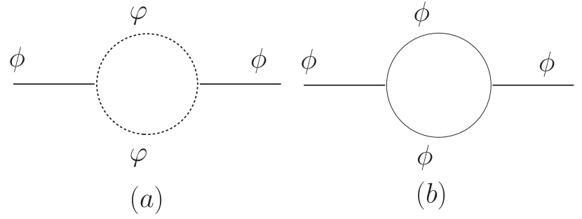
Figure 1: Self energies: Fig.(a) depicts the self energy contribution from a loop of $\varphi$ particles, Fig. (b) depicts the self-energy from the self-interaction of the inflaton.

It is clear from these figures that we only need to obtain the self-energy in only one of the cases, since one case is obtained from the other by a simple replacement of the masses of the particles that run in the loop. Therefore, we will study the self-energy for the case of figure fig. 1 a.

It is convenient to pass to conformal time $\eta$ with $d\eta=dt/a(t)$ and introduce a conformal rescaling of the fields

$$a(t)\;\phi(\vec{x},t)=\chi(\vec{x},\eta)~{}~{};~{}~{}a(t)\;\varphi(\vec{x},t)=\delta(\vec{x},\eta)$$ (6)

The action Eq. (4) (after discarding surface terms that do not affect the equations of motion) reads:

$$A\Big{[}\chi,\delta\Big{]}=\int d^{3}x\;d\eta\;\Bigg{\{}\frac{{\chi^{\prime}}^{2}}{2}-\frac{(\nabla\chi)^{2}}{2}-\frac{\mathcal{M}^{2}_{\chi}(\eta)}{2}\;\chi^{2}+\frac{{\delta^{\prime}}^{2}}{2}-\frac{(\nabla\delta)^{2}}{2}-\frac{\mathcal{M}^{2}_{\delta}(\eta)}{2}\;\delta^{2}-g\;C(\eta)\;\chi\;\delta^{2}+C^{3}(\eta)\;J(\eta)\;\chi\Bigg{\}}$$ (7)

with primes denoting derivatives with respect to conformal time $\eta,\;C(\eta)=a(t(\eta))$ is the scale factor as a function of $\eta$ and

$$\mathcal{M}^{2}_{\chi}(\eta)=M^{2}\;C^{2}(\eta)-\frac{C^{\prime\prime}(\eta)}{C(\eta)}\quad,\quad\mathcal{M}^{2}_{\delta}(\eta)=m^{2}\;C^{2}(\eta)-\frac{C^{\prime\prime}(\eta)}{C(\eta)}\;.$$ (8)

In this section we focus on a de Sitter inflationary cosmology, we treat slow-roll and quasi de Sitter inflation in sec. IV. For de Sitter space time the scale factor is given by

$$a(t)=e^{Ht}\quad,\quad C(\eta)=-\frac{1}{H\eta}\;,$$ (9)

with $H$ the Hubble constant and the conformal time $\eta$ is given by

$$\eta=-\frac{e^{-Ht}}{H}\;,$$ (10)

where $\eta=-\frac{1}{H}$ corresponds to the initial time $t=0$.

The Heisenberg equations of motion for the Fourier field modes of wave vector $k$ in the free ($g=0$) theory are given by

$$\chi^{\prime\prime}_{\vec{k}}(\eta)+\Big{[}k^{2}-\frac{1}{\eta^{2}}\Big{(}\nu^{2}-\frac{1}{4}\Big{)}\Big{]}\chi_{\vec{k}}(\eta) = 0\;,$$ (11)

$$\delta^{\prime\prime}_{\vec{k}}(\eta)+\Big{[}k^{2}-\frac{1}{\eta^{2}}\Big{(}\bar{\nu}^{2}-\frac{1}{4}\Big{)}\Big{]}\delta_{\vec{k}}(\eta) = 0$$ (12)

where

$$\nu^{2}=\frac{9}{4}-\frac{M^{2}}{H^{2}}\quad,\quad\bar{\nu}^{2}=\frac{9}{4}-\frac{m^{2}}{H^{2}}\;.$$ (13)

The Heisenberg free field operators can be expanded in terms of the linearly independent solutions of the mode equation

$$S^{\prime\prime}_{\nu}(k;\eta)+\Big{[}k^{2}-\frac{1}{\eta^{2}}\Big{(}\nu^{2}-\frac{1}{4}\Big{)}\Big{]}S_{\nu}(k;\eta)=0\,,$$ (14)

for $\nu,\bar{\nu}$ respectively. We choose the usual Bunch-Davies initial conditions for the mode functions, namely the usual plane waves for wavelengths deep inside the Hubble radius $|k\;\eta|\gg 1$. The mode functions $S_{\nu}(q,\eta)$ associated with the Bunch-Davies vacuum are given by

$$S_{\bar{\nu}}(k,\eta)=\frac{1}{2}\;i^{-\nu-\frac{1}{2}}\sqrt{\pi\eta}\;H^{(2)}_{\nu}(k\eta)\;.$$ (15)

For wavelengths much smaller than the Hubble radius, ( $|k\eta|\gg 1$) the mode functions with Bunch-Davies vacuum initial condition behave as plane waves in Minkowski space time, namely

$$S_{\nu}(k;\eta)\buildrel|k\eta|\gg 1\over{=}\frac{1}{\sqrt{2k}}\,e^{-ik\eta}\;.$$ (16)

In particular for $\nu=3/2$, eq.(15) becomes

$$S_{\frac{3}{2}}(k,\eta)=\frac{1}{\sqrt{2k}}\;e^{-ik\,\eta}\left[1-\frac{i}{k\eta}\right]\;.$$ (17)

The spatial Fourier transform of the free Heisenberg field operators $\chi_{\vec{k}}(\eta),\;\delta_{\vec{k}}(\eta)$ are therefore written as

$$\chi_{\vec{k}}(\eta) = \alpha_{\vec{k}}\;S_{\nu}(k;\eta)+\alpha^{\dagger}_{-\vec{k}}\;S^{*}_{\nu}(k;\eta)$$ (18)

$$\delta_{\vec{k}}(\eta) = \beta_{\vec{k}}\;S_{\bar{\nu}}(k;\eta)+\beta^{\dagger}_{-\vec{k}}\;S^{*}_{\bar{\nu}}(k;\eta)$$ (20)

where the Heisenberg operators $\alpha_{\vec{k}};\alpha^{\dagger}_{\vec{k}}$ and $\beta_{\vec{k}};\beta^{\dagger}_{\vec{k}}$ obey the usual canonical commutation relations. The Bunch-Davies vacuum state $|0\rangle$ is annihilated by $\alpha_{\vec{k}},\beta_{\vec{k}}$.

III Equations of motion, dynamical renormalization group and decay laws: the $\Delta$ expansion in de Sitter inflation.

As described in detail in desiterI , in a rapidly expanding cosmology the notion of decay ‘rate’ requires a careful analysis. In Minkowski space time the decay rate is obtained from the transition probability per unit time, or alternatively from the imaginary part of the space-time Fourier transform of the self-energy evaluated on the particle’s mass shell. In the transition probability, the square of the energy-momentum delta functions accounts for the space-time volume times an overall delta function of energy-momentum conservation: the transition probability divided by this volume is the decay rate. In Minkowski space-time, the self-energy is a function of the difference of the space-time coordinates due to translational invariance. Hence, a space-time Fourier transform is available, from which the imaginary part is extracted. Energy-momentum conservation is of paramount importance to define the decay rate in Minkowski space-time, and to determine the kinematic thresholds for particle production and decay.

In a rapidly expanding cosmology the lack of a global time-like Killing vector prevents energy momentum conservation, although energy is covariantly conserved. As a result: i) a new definition of the decay ‘rate’ that does not rely on energy-momentum conservation, and a different approach to studying the decay law is necessary ii) since energy is no longer conserved, novel processes are possible which are forbidden in Minkowski space-time, therefore we expect novel decay channels which are absent in Minkowski space-time.

In ref.desiterI the decay of a particle into massless conformally coupled particles was studied as a test example to present the main concepts: the mode functions are the same as in Minkowski space time, this simplified the calculation of the self-energy kernel, allowed a systematic study of the reliability of the dynamical renormalization group method and a direct comparison to the Minkowski limit. This simple case, however, does not feature several important aspects of the more relevant situation of the dynamics of quantum fields which are massless or nearly so but minimally coupled to gravity. This latter case features infrared divergences which are not present in the simpler case of conformally coupled massless fields prem ; IRcosmo . In this article we study the case in which the inflaton is massive and minimally coupled to gravity which is precisely the relevant case for studying the decay of quantum fluctuations during slow roll inflation.

While the main aspects of the dynamical renormalization group method to study decay were introduced in desiterI , we briefly highlight here the main aspects relevant to this work.

The method relies on studying the real time relaxation of the expectation value of a field induced by an external source in linear response: as the source is switched-off the expectation value relaxes revealing the decay law of the amplitude. While an exact solution of the equations of motion is readily available in Minkowski space time because the self-energy is a function of the difference of the time coordinates (allowing the use of Fourier-Laplace transforms), this is , in general, not the case during inflation. Solving the equation of motion in a perturbative expansion in the coupling, secular terms emerge, these terms grow in time when the conformal time $\eta\rightarrow 0$, limiting the validity of the perturbative expansion. The dynamical renormalization group precisely allows a systematic resummation of these secular terms and the uniform asymptotic expansion provided by the resummation lead to the identification of the decay law of the amplitude. Thus, the main steps of the method are the following:

• First, obtain the (retarded) equations of motion for the expectation value of the field in linear response after switching-off the source that induces the expectation value.

• Second, obtain a perturbative expansion of the solution in terms of the coupling. Such perturbative solution features secular terms, namely terms that grow in time (when conformal time $\eta\rightarrow 0$ during inflation) and limit the validity of the perturbative expansion.

• Third, implement the dynamical renormalization group (DRG) to provide a systematic resummation of these secular terms. The solution of the DRG equation gives the decay law of the amplitude of quantum fluctuations.

We implement these steps in the general case described by the action Eq. (4) which couples two fields: $\phi$ and $\varphi$ with masses $M$ and $m$, respectively and a cubic coupling $g\phi\,\varphi^{2}$ in exact de Sitter space-time. In section IV we apply these results to the case of the self-coupling of inflaton fluctuations.

We focus on obtaining the decay law for the quantum fluctuations of the field $\phi$ which will be later identified with the inflaton field. We derive the equation of motion for the expectation value of the field using the non-equilibrium generating functional which involves forward and backward time evolution, typical of a density matrix. Unlike the S-matrix case (which is an in-out transition where only forward time evolution is required), the time evolution of an expectation value is an initial value problem which requires an in-in matrix element. Real time equations of motion obtained from the non-equilibrium generating functional are guaranteed to be retarded.

It is convenient to write the spatial Fourier transform of the conformally re-scaled field $\chi$ as follows

$$\chi^{\pm}_{\vec{k}}(\eta)=X_{\vec{k}}(\eta)+\sigma^{\pm}_{\vec{k}}(\eta)~{}~{};~{}~{}\langle\chi^{\pm}_{\vec{k}}(\eta)\rangle=X_{\vec{k}}(\eta)~{}~{};~{}~{}\langle\sigma^{\pm}_{\vec{k}}(\eta)\rangle=0$$ (21)

where the superscripts $\pm$ refer to the forward and backward time branches in the non-equilibrium generating functional respectively. The expectation value is the same for both branches since the c-number external source is the same. The equation of motion for the expectation value $X_{\vec{k}}(\eta)$ is obtained by requiring $\langle\sigma^{\pm}_{\vec{k}}(\eta)\rangle=0$ systematically order by order in perturbation theory. This is the basis of the tadpole method to obtain the equations of motion, which up to $\mathcal{O}(g^{2})$ (one-loop) are given by [see Eq.(37) in ref.desiterI ]

$$X^{\prime\prime}_{\vec{k}}(\eta)+\left[k^{2}-\frac{\nu^{2}-\frac{1}{4}}{\eta^{2}}\right]X_{\vec{k}}(\eta)+\frac{2\;g^{2}}{\eta\;H^{2}}\;\int_{\eta_{0}}^{\eta}\frac{d\eta^{\prime}}{\eta^{\prime}}\;\mathcal{K}_{\bar{\nu}}(k;\eta,\eta^{\prime})\;X_{\vec{k}}(\eta^{\prime})=0\;,$$ (22)

where the counterterm $J(\eta)$ in the action (7) has been used to cancel the tadpole term proportional to $\langle\delta^{2}(\vec{x},\eta)\rangle$, this is independent of $X_{\vec{k}}(\eta)$ and acts as a source term in the equation of motion. $\nu$ and $\bar{\nu}$ are given by Eq.(13 ).

The retarded one-loop self-energy kernel $\mathcal{K}_{\bar{\nu}}(k;\eta,\eta^{\prime})$ is given by desiterI

$$\mathcal{K}_{\bar{\nu}}(k;\eta,\eta^{\prime})=2\int\frac{d^{3}q}{(2\pi)^{3}}\;\mathrm{Im}\left[S_{\bar{\nu}}(q,\eta)S^{*}_{\bar{\nu}}(q,\eta^{\prime})S_{\bar{\nu}}(|\vec{q}-\vec{k}|,\eta)S^{*}_{\bar{\nu}}(|\vec{q}-\vec{k}|,\eta^{\prime})\right]$$ (23)

and is depicted in fig. 1-a. The mode functions $S_{\bar{\nu}}(q,\eta)$ are given by Eq. (15). We consider $M^{2}/H^{2}\ll 1$ and $m^{2}/H^{2}\ll 1$ which for the inflaton case to be studied below corresponds to the slow-roll approximation, and define

$$\Delta\equiv\frac{3}{2}-\bar{\nu}\quad,\quad\Delta=\frac{1}{3}\frac{m^{2}}{H^{2}}+\mathcal{O}\left(\frac{m^{4}}{H^{4}}\right)$$ (24)

hence $\Delta\ll 1$. This small parameter $\Delta$ will be related with the slow-roll parameters and plays an important role in regulating the infrared behavior in the self-energy. Anticipating a renormalization of the inflaton mass we write

$$M^{2}=M^{2}_{R}+g^{2}\;\delta M^{2}_{1}+\mathcal{O}(g^{4})\Rightarrow\nu^{2}=\nu^{2}_{R}-g^{2}\;\frac{\delta M^{2}_{1}}{H^{2}}+\mathcal{O}(g^{4})\;,$$ (25)

with $\nu^{2}_{R}=9/4-M^{2}_{R}/H^{2}$. The equation of motion up to order $g^{2}$ becomes

$$X^{\prime\prime}_{\vec{k}}(\eta)+\left[k^{2}-\frac{\nu^{2}_{R}-\frac{1}{4}}{\eta^{2}}\right]X_{\vec{k}}(\eta)+g^{2}\frac{\delta M^{2}_{1}}{H^{2}\,\eta^{2}}X_{\vec{k}}(\eta)+\frac{2\,g^{2}}{\eta\;H^{2}}\;\int_{\eta_{0}}^{\eta}\frac{d\eta^{\prime}}{\eta^{\prime}}\;\mathcal{K}_{\bar{\nu}}(k;\eta,\eta^{\prime})\;X_{\vec{k}}(\eta^{\prime})=0\;,$$ (26)

In what follows we suppress the subscript $R$ to avoid cluttering the notation, therefore $\nu$ and the mass must be understood as the renormalized ones. A perturbative solution of Eq.(22) is obtained by writing

$$X_{\vec{k}}(\eta)=X_{0,\vec{k}}(\eta)+g^{2}\;X_{1,\vec{k}}(\eta)+\mathcal{O}(g^{4})$$ (27)

and comparing powers of $g$ leads to a hierarchy of coupled equations: up to second order in $g$, (one loop order), they are

$$X^{\prime\prime}_{0,\vec{k}}(\eta)+\left[k^{2}-\frac{1}{\eta^{2}}\Big{(}\nu^{2}-\frac{1}{4}\Big{)}\right]X_{0,\vec{k}}(\eta)=0\;,$$ (28)

$$X^{\prime\prime}_{1,\vec{k}}(\eta)+\left[k^{2}-\frac{1}{\eta^{2}}\Big{(}\nu^{2}-\frac{1}{4}\Big{)}\right]X_{1,\vec{k}}(\eta)=\mathcal{R}_{1}(k,\eta)\;,$$ (29)

where the inhomogeneity is given by

$$\mathcal{R}_{1}(k,\eta)=-\frac{\delta M^{2}_{1}}{H^{2}\,\eta^{2}}\;X_{0,\vec{k}}(\eta)-\frac{2}{H^{2}\;\eta}\int_{\eta_{0}}^{\eta}\frac{d\eta^{\prime}}{\eta^{\prime}}\;\mathcal{K}_{\bar{\nu}}(k;\eta,\eta^{\prime})\;X_{0,\vec{k}}(\eta^{\prime})\;.$$ (30)

The mass counterterm $\delta M^{2}_{1}$ is fixed by requiring that it cancels the term proportional to $X_{0,\vec{k}}(\eta)/\eta^{2}$ arising from the integral in Eq.(30). The first order correction to the solution is given by

$$X_{1,\vec{k}}(\eta)=\int_{\eta_{0}}^{0}d\eta^{\prime}\;\mathcal{G}_{\nu}(k;\eta,\eta^{\prime})\;\mathcal{R}_{1}(k,\eta^{\prime})\;.$$ (31)

where $\mathcal{G}(k;\eta,\eta^{\prime})$ is the retarded Green’s function obeying

$$\left[\frac{d^{2}}{d\eta^{2}}+k^{2}-\frac{1}{\eta^{2}}\Big{(}\nu^{2}-\frac{1}{4}\Big{)}\right]\mathcal{G}_{\nu}(k;\eta,\eta^{\prime})=\delta(\eta-\eta^{\prime})~{}~{},~{}~{}\mathcal{G}_{\nu}(k;\eta,\eta^{\prime})=0\quad\mathrm{for}\quad\eta^{\prime}>\eta\;.$$ (32)

To compute $X_{1,\vec{k}}(\eta)$ we first need the kernel $\mathcal{K}_{\bar{\nu}}(k;\eta,\eta^{\prime})$. As it will become clear in the following, this kernel involves (logarithmic) infrared divergences for $\bar{\nu}=3/2$, but it is an analytic function of $\Delta$ that features simple poles at $\Delta=0$. Since in slow roll $\Delta\ll 1$ we will use the parameter $\Delta$ as a regulator much in the same manner as the $\varepsilon$ expansion in dimensional regularization. We will therefore compute the kernel $\mathcal{K}_{\bar{\nu}}(k;\eta,\eta^{\prime})$ at leading order in $\Delta$ by extracting the poles and the logarithmic terms; terms proportional to powers of $\Delta$ give subleading contributions. This is akin to the minimal subtraction in dimensional regularization.

III.1 Secular terms, DRG and decay law:

Let $g_{\nu}(k,\eta)$ and $f_{\nu}(k,\eta)$ be two independent solutions of the zeroth order equation (28), the most general solution is

$$X_{0,\vec{k}}(\eta)=A_{\vec{k}}\;g_{\nu}(k,\eta)+B_{\vec{k}}\;f_{\nu}(k,\eta)$$ (33)

where $A_{\vec{k}}$ and $B_{\vec{k}}$ are arbitrary constants. The linear structure of the perturbative series indicates that the perturbative solution of the equation of motion has the form

$$X_{\vec{k}}(\eta)=A_{\vec{k}}\;g_{\nu}(k,\eta)[1+g^{2}\;F_{1}(k,\eta)+\mathcal{O}(g^{4})]+B_{\vec{k}}\;f_{\nu}(k,\eta)[1+g^{2}\;H_{1}(k,\eta)+\mathcal{O}(g^{4})]$$ (34)

The functions $F_{1}(k,\eta);\;H_{1}(k,\eta)$ are determined by the first order solution Eq.(31) and they feature secular terms, namely divergent terms in the limit $\eta\rightarrow 0$. Therefore we write,

$$F_{1}(k;\eta)=F_{1,s}(k;\eta)+F_{1,f}(k;\eta)~{}~{};~{}~{}H_{1}(k;\eta)=H_{1,s}(k;\eta)+H_{1,f}(k;\eta)$$ (35)

where $F_{1,s}(k;\eta),H_{1,s}(k;\eta)$ are secular terms, whereas $F_{1,f}(k;\eta),H_{1,f}(k;\eta)$ remain bounded as functions of conformal time. The dynamical renormalization group absorbs the secular terms into a renormalization of the amplitudes $A_{\vec{k}},B_{\vec{k}}$ at a given time scale $\widetilde{\eta}$, (wave-function renormalization) desiterI ; DRG , namely

$$A_{\vec{k}} = A_{\vec{k}}(\widetilde{\eta})\;Z^{A}_{\vec{k}}(\widetilde{\eta})\quad,\quad Z^{A}_{\vec{k}}(\widetilde{\eta})=1+g^{2}\;z^{A}_{1,\vec{k}}(\widetilde{\eta})+\mathcal{O}(g^{4})$$ (36)

$$B_{\vec{k}} = B_{\vec{k}}(\widetilde{\eta})\;Z^{B}_{\vec{k}}(\widetilde{\eta})\quad,\quad Z^{B}_{\vec{k}}(\widetilde{\eta})=1+g^{2}\;z^{B}_{1,\vec{k}}(\widetilde{\eta})+\mathcal{O}(g^{4})$$ (37)

The coefficients $z^{A}_{1,\vec{k}}(\widetilde{\eta}),\;z^{B}_{1,\vec{k}}(\widetilde{\eta})$ are chosen to cancel the secular terms in the perturbative solution at $\eta=\widetilde{\eta}$ order by order in the perturbative expansion. Since the scale $\widetilde{\eta}$ is arbitrary and the perturbative solution does not depend on this scale, the renormalized amplitudes $A_{\vec{k}}(\widetilde{\eta}),\;B_{\vec{k}}(\widetilde{\eta})$ obey the following dynamical renormalization group equation to lowest order (Eqs.(55)-(56) of ref.desiterI ; DRG ),

$$\frac{\partial A_{\vec{k}}(\widetilde{\eta})}{\partial\widetilde{\eta}}-g^{2}\;A_{\vec{k}}(\widetilde{\eta})\;\frac{\partial F_{1,s}(k;\widetilde{\eta})}{\partial\widetilde{\eta}}+\mathcal{O}(g^{4}) = 0$$ (38)

$$\frac{\partial B_{\vec{k}}(\widetilde{\eta})}{\partial\widetilde{\eta}}-g^{2}\;B_{\vec{k}}(\widetilde{\eta})\;\frac{\partial H_{1,s}(k;\widetilde{\eta})}{\partial\widetilde{\eta}}+\mathcal{O}(g^{4}) = 0$$ (39)

The solution of these DRG equations is given by

$$A_{\vec{k}}(\widetilde{\eta})=A_{\vec{k}}(\widetilde{\eta}_{0})\;e^{g^{2}\left[F_{1,s}(k;\widetilde{\eta})-F_{1,s}(k;\widetilde{\eta}_{0})\right]+\mathcal{O}(g^{4})}\quad,\quad B_{\vec{k}}(\widetilde{\eta})=B_{\vec{k}}(\widetilde{\eta}_{0})\;e^{g^{2}\left[H_{1,s}(k;\widetilde{\eta})-H_{1,s}(k;\widetilde{\eta}_{0})\right]+\mathcal{O}(g^{4})}$$ (40)

Setting $\widetilde{\eta}=\eta$ we obtain the renormalization group improved solution,

$$X_{\vec{k}}(\eta) = A_{\vec{k}}({\eta})\;\,g_{\nu}(k;\eta)\left[1+g^{2}\;F_{1,f}(k,\eta)+\mathcal{O}(g^{4})\right]+B_{\vec{k}}({\eta})\;f_{\nu}(k;\eta)\left[1+g^{2}\;H_{1,f}(k,\eta)+\mathcal{O}(g^{4})\right]$$ (41)

$$A_{\vec{k}}({\eta}) = A_{\vec{k}}({\eta}_{0})~{}e^{g^{2}\left[F_{1,s}(k;{\eta})-F_{1,s}(k;{\eta}_{0})\right]}\quad,\quad B_{\vec{k}}({\eta})=B_{\vec{k}}({\eta}_{0})~{}e^{g^{2}\left[H_{1,s}(k;{\eta})-H_{1,s}(k;{\eta}_{0})\right]}\;.$$ (42)

The terms in the brackets in Eq. (41) are truly perturbatively small at all conformal times. The real part of the exponential factors in the complex amplitudes Eq. (42) determine the decay law of the amplitude (or growth law in the case of instabilities).

III.2 The $\Delta$ expansion:

When the inflaton decays into minimally coupled massless particles, infrared divergences in the self-energy kernel are present prem . These divergences are a hallmark of minimally coupled massless particles namely $\bar{\nu}=\nu=3/2$ in the intermediate state, and are similar to those found for gravitons in de Sitter space-timeIRcosmo . We are instead considering the case in which both the inflaton and the decay products are massive with masses $M$ and $m$ respectively and $(M^{2}/H^{2},m^{2}/H^{2})\ll 1$. The mass of the particles in the loop cutoffs the infrared divergences here, (since $m^{2}/H^{2}\neq 0$ then $\bar{\nu}\neq 3/2$ and $\Delta\neq 0$ [Eq. (24)]). As it will become clear in the explicit calculations below, the infrared divergences in the self-energy kernel manifest as simple poles at $\Delta=0$. Thus, $0<\Delta\ll 1$ emerges as an infrared regulator akin to the dimensional regularization parameter $\varepsilon=4-D$ in the loop expansion in D-dimensional Minkowski space-time.

Since $\Delta\ll 1$ for slow roll inflation, we compute the self-energy kernel in an expansion in $\Delta$ keeping the poles at $\Delta=0$ and the leading logarithms in $\eta$ just like the $\varepsilon$ expansion in dimensional regularization. (The leading $\log\eta$ terms are the remnant of the infrared divergence regulated by $\Delta$ just like in the $\varepsilon$ expansion of critical phenomena).

The details of the calculation of $\mathcal{K}_{\bar{\nu}}(k,\eta,\eta^{\prime})$ in the $\Delta$-expansion for arbitrary $k$ is presented in the appendix and the result for the kernel is given by equations (B) and (B). We now have all the elements necessary to study the decay law.

III.3 Superhorizon modes: $k=0$

We begin by the superhorizon modes and take $k=0$. The general solution of the unperturbed mode Eq.(28) and the retarded Green’s function $\mathcal{G}_{\nu}(0,\eta,\eta^{\prime})$ Eq. (32) for $k=0$ are given by

$$X_{0,\vec{0}}(\eta) = A\;(-\eta)^{\beta_{+}}+B\;(-\eta)^{\beta_{-}}\;;\;\beta_{\pm}=\frac{1}{2}\pm\nu.$$ (43)

$$\mathcal{G}_{\nu}(0,\eta,\eta^{\prime}) = \frac{1}{2\nu}\left[(-\eta)^{\beta_{+}}\;(-\eta^{\prime})^{\beta_{-}}-(-\eta)^{\beta_{-}}\;(-\eta^{\prime})^{\beta_{+}}\right]\Theta(\eta-\eta^{\prime})$$ (44)

We compute the kernel $\mathcal{K}_{\bar{\nu}}(0,\eta,\eta^{\prime})$ in Appendix A highlighting the most relevant physical processes and displaying the origin of infrared divergences as poles at $\Delta=0$ and the leading logarithms in $\eta$. $\mathcal{K}_{\bar{\nu}}(0,\eta,\eta^{\prime})$ can also be obtained in the limit $k\rightarrow 0$ of the $k\neq 0$ kernel treated in Appendix B [Eq.(B)].

For $k=0$ the self-energy kernel is given by

$$\mathcal{K}_{\bar{\nu}}(0;\eta,\eta^{\prime})=\frac{1}{\pi^{2}}\int_{0}^{\infty}q^{2}\;dq~{}\mathrm{Im}\left\{\left[S_{\bar{\nu}}(q,\eta)S^{*}_{\bar{\nu}}(q,\eta^{\prime})\right]^{2}\right\}\quad,\quad\bar{\nu}=\frac{3}{2}-\Delta\;.$$ (45)

The infrared divergences at $\Delta=\frac{3}{2}-\bar{\nu}=0$ arise from the small momenta behavior of the integrand in Eq.(45). Keeping $\Delta$ small but nonzero, we find for the kernel (see appendix A)

$$\mathcal{K}_{\bar{\nu}}(0;\eta,\eta^{\prime})=\mathcal{K}_{\frac{1}{2}}(0;\eta,\eta^{\prime})+\frac{1}{6\pi^{2}}\Bigg{\{}\left[\frac{1}{2\Delta}+\frac{2}{3}\right]\left(\frac{\eta^{\prime}}{\eta^{2}}-\frac{\eta}{\eta^{{}^{\prime}2}}\right)-\frac{\eta^{\prime}}{\eta^{2}}\ln\left(\frac{\eta^{\prime}}{\eta}\right)+\left(\frac{\eta}{\eta^{{}^{\prime}2}}-\frac{\eta^{\prime}}{\eta^{2}}\right)\ln\left[1-\frac{\eta}{\eta^{\prime}}\right]+\frac{1}{\eta^{\prime}}-\frac{1}{\eta}\Bigg{\}}$$ (46)

where

$$\mathcal{K}_{\frac{1}{2}}(0;\eta,\eta^{\prime})=-\frac{1}{8\pi^{2}}\;\mathcal{P}\left(\frac{1}{\eta-\eta^{\prime}}\right)=-\frac{1}{8\pi^{2}}\;\frac{\eta-\eta^{\prime}}{\left(\eta-\eta^{\prime}\right)^{2}+(\epsilon\;\eta^{\prime})^{2}}=-\frac{1}{8\pi^{2}}\;\frac{1}{2}\left[\frac{1}{\eta-\eta^{\prime}+i\epsilon\;\eta^{\prime}}+\frac{1}{\eta-\eta^{\prime}-i\epsilon\;\eta^{\prime}}\right]~{}~{};~{}~{}\epsilon\rightarrow 0\;.$$ (47)

This prescription for the principal part regulates the short distance divergence in the operator product expansion with a dimensionless infinitesimal $\epsilon$ independent of time. This choice of regularization is consistent with the short-distance singularities of the operator product expansion in Minkowski space-time, and leads to a time-independent mass renormalization (see also ref. desiterI ).

The two terms in the Eq.(46), namely $\mathcal{K}_{\frac{1}{2}}(0;\eta,\eta^{\prime})$ and the term in braces have very different origin. $\mathcal{K}_{\frac{1}{2}}(0;\eta,\eta^{\prime})$ accounts for the large loop momentum contribution $q\eta,q\eta^{\prime}\gg 1$ where the behavior of the mode functions is the same as for conformally coupled massless fields, in particular, the short distance (ultraviolet) divergence is present only in this term. The terms in the braces account for the strong infrared behavior of superhorizon wavelengths reflected by the pole at $\Delta=0$ and the logarithms in $\eta$. This calculation exhibits clearly the origin of the different contributions.

Figure 2: Decay of the field $\phi$ (solid line) for $k=0$ into superhorizon modes of the field $\varphi$

(dashed lines)

It remains to integrate over $\eta^{\prime}$ in the second term in Eq. (30) with the kernel given by Eq.(46). The integral involving $\mathcal{K}_{\frac{1}{2}}(0;\eta,\eta^{\prime})$ in Eq.(46) was given in ref.desiterI . The integrals over $\eta^{\prime}$ for the second term (between braces) in Eq.(46) can be done easily by expanding the $\ln[1-\eta/\eta^{\prime}]$ in a power series in $\eta/\eta^{\prime}$ and integrating term by term. The result of the integral over $\eta^{\prime}$ in Eq. (30) is of the form

$$\frac{2}{H^{2}\;\eta}\int_{\eta_{0}}^{\eta}\frac{d\eta^{\prime}}{\eta^{\prime}}\;\mathcal{K}_{\bar{\nu}}(0;\eta,\eta^{\prime})\;X_{0,0}(\eta^{\prime})=A\;(-\eta)^{\beta_{+}}\;\frac{\alpha_{+}}{\eta^{2}}+B\;(-\eta)^{\beta_{-}}\;\frac{\alpha_{-}}{\eta^{2}}+F[\eta,\eta_{0}]$$ (48)

where $F[\eta,\eta_{0}]$ refers to the contribution of the lower integration limit and does not produce secular terms in $X_{\vec{0}}(\eta)$.

Integrating over $\eta^{\prime}$ in Eq.(48) yields,

$$\alpha_{+}=\frac{1}{(2\,\pi\,H)^{2}}\left[\ln\epsilon+\gamma+\psi(\frac{1}{2}-\nu)\right]+\frac{1}{3(\pi\,H)^{2}}\left[\frac{1}{\nu^{2}-\frac{9}{4}}\left(\frac{3}{2\,\Delta}+2-3\,\gamma\right)+\frac{1}{\nu^{2}-\frac{1}{4}}+\frac{1}{(\nu+\frac{3}{2})^{2}}+\frac{\psi(\frac{5}{2}-\nu)}{\frac{3}{2}-\nu}+\frac{\psi(-\frac{1}{2}-\nu)}{\frac{3}{2}+\nu}\right]\;.$$ (49)

where we used Eq.(46), $\gamma$ is the Euler-Mascheroni constant, and the contribution from $\mathcal{K}_{\frac{1}{2}}(0,\eta,\eta^{\prime})$ desiterI . $\alpha_{-}$ follows from $\alpha_{+}$ by changing $\nu\to-\nu$ while $\bar{\nu}$ is unchanged. Introducing the symmetric and antisymmetric combinations,

$$\alpha_{s}=\frac{1}{2}\left[\alpha_{+}+\alpha_{-}\right]\quad,\quad\alpha_{a}=\frac{1}{2}\left[\alpha_{+}-\alpha_{-}\right]\;,$$ (50)

the symmetric term,

$$\left[A\;(-\eta)^{\beta_{+}}+B\;(-\eta)^{\beta_{-}}\right]\;\frac{\alpha_{s}}{\eta^{2}}=\frac{X_{0,\vec{0}}(\eta)}{\eta^{2}}\;\alpha_{s}$$ (51)

is identified with a contribution to mass renormalization and is cancelled by the counterterm $\delta M^{2}_{1}$ including the logarithmic ultraviolet divergence $\ln\epsilon$ [$\epsilon$ the short distance regulator Eq. (47)]. Eqs.(49) and (50) yield,

$$\alpha_{a}=\frac{1}{8\pi\,H^{2}}\tan[\pi\,\nu]\left[1+\frac{4}{\frac{9}{4}-\nu^{2}}\right]\;.$$ (52)

The unit term in the bracket arises from the contribution of $\mathcal{K}_{\frac{1}{2}}(0,\eta,\eta^{\prime})$. After cancelling the term given by Eq. (51) with a proper choice of the mass counterterm, and taking into account that $F[\eta,\eta_{0}]$ does not contribute to the secular terms, we find the solution of the equation of motion up to $\mathcal{O}(g^{2})$

$$X_{\vec{0}}(\eta)=X_{0,\vec{0}}(\eta)\left[1+\Gamma\;\ln\frac{\eta}{\eta_{0}}+\mathrm{non-secular~{}terms}\right]$$ (53)

with

$$\Gamma=\frac{g^{2}}{16\pi\,H^{2}\,\nu}\tan[\pi\,\nu]\left[1+\frac{4}{\frac{9}{4}-\nu^{2}}\right]=\frac{g^{2}}{16\pi\,H^{2}\,\nu}\tan[\pi\,\nu]\left[1+\frac{4\,H^{2}}{M^{2}}\right]~{}~{},~{}~{}\nu=\sqrt{\frac{9}{4}-\frac{M^{2}}{H^{2}}}\;.$$ (54)

The dynamical renormalization group resummation exponentiates the secular terms in Eq.(53) [see Eqs.(41)-(42)] and leads to the improved solution,

$$X_{\vec{0}}(\eta)=\left[\frac{\eta}{\eta_{0}}\right]^{\Gamma}\Bigg{\{}A(\eta_{0})\;(-\eta)^{\beta_{+}}[1+\mathcal{O}(g^{2})]+B({\eta}_{0})\;(-\eta)^{\beta_{-}}[1+\mathcal{O}(g^{2})]\Bigg{\}}\;.$$ (55)

The first term inside the square bracket in Eq. (54) (namely the unit term) corresponds to the case in which the inflaton decays into massless particles conformally coupled to gravity desiterI ,prem .

The calculation leading to eq.(54) is valid for $\bar{\nu}\to\frac{3}{2}$ (namely, $m\ll H$) and we keep $\nu$ as well as $M$ arbitrary. We can analytically continue the formula (54) to $H<M$ and then take the $m\ll H\ll M$ limit. In this limit $\Gamma$ becomes the decay rate of a particle with mass $M$ into massless particles in Minkowski space-time:

$$\lim_{m\ll H\to 0}H\;\Gamma=\Gamma_{Mink}=g^{2}/(16\pi M)\quad,$$

as it must be.

III.4 Modes inside the horizon during inflation: $|k\eta|\gg 1$

The kernel $\mathcal{K}_{\bar{\nu}}(k;\eta,\eta^{\prime})$ for arbitrary $k$ has been computed in the appendix in leading order in the $\Delta$ expansion and up to leading logarithms. It is given by equations (B) and (B). Obtaining the perturbative solution and extracting the secular terms leading to the decay law for arbitrary $k$ is an extremely difficult task which requires a full numerical study. However, explicit expressions can be derived for wavelengths deep inside the Hubble radius all throughout inflation, namely $|k\eta|,|k\eta^{\prime}|>>1$. In the appendix we show that in the short wavelength limit the kernel simplifies to the following expression [Eq. (167)]

$$\mathcal{K}_{\bar{\nu}}(k,\eta,\eta^{\prime})=\mathcal{K}_{\frac{1}{2}}(k,\eta,\eta^{\prime}) - \frac{1}{4\pi^{2}k\eta\eta^{\prime}}\Bigg{\{}\sin k(\eta-\eta^{\prime})\left[\frac{1}{\Delta}+\mathcal{C}-\ln k(\eta-\eta^{\prime})+\ln k^{2}\eta\eta^{\prime}-\mathrm{Ci}[2k(\eta-\eta^{\prime})]\right]+$$ (56)

$$+\cos k(\eta-\eta^{\prime})\left[\frac{\pi}{2}+\mathrm{Si}[2k(\eta-\eta^{\prime})]\right]\Bigg{\}}\;,$$

where $\mathcal{C}=\ln 2+\gamma-2$. Again, the first term in this expression is the self-energy kernel for conformally coupled massless fields in the loop,

$$\mathcal{K}_{\frac{1}{2}}(k,\eta,\eta^{\prime})=-\frac{1}{8\pi^{2}}\;\cos k(\eta-\eta^{\prime})\;\mathcal{P}\left(\frac{1}{\eta-\eta^{\prime}}\right)\;.$$ (57)

The principal part is defined by Eq. (47). A close examination of the steps leading to this expression in the appendix shows that this contribution originates solely from the high loop momenta $q\eta,q\eta^{\prime}\gg 1$ for which the mode functions coincide with those of massless conformally coupled fields. The second term within brackets which features the $1/\Delta$ and the logarithms originate in the process of emission of superhorizon modes. Two regions in the integral over the loop momentum $q$ give rise to these contributions: $q\ll 1/\eta$ and $|\vec{k}-\vec{q}|\ll 1/\eta$, corresponding to the case when either line in the loop transfers very small momentum (superhorizon modes). These processes can be described as bremsstrahlung radiation of superhorizon quanta and are depicted in fig. 3.

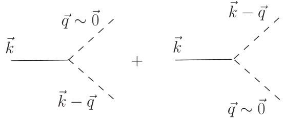
Figure 3: Infrared contributions to $\phi\rightarrow\varphi\varphi$. The external particle has a wavelength deep inside the horizon but one of the intermediate lines has superhorizon wavelengths. This process is identified as bremsstrahlung radiation of superhorizon quanta.

This process is analogous to the generation of Hawking radiation from black holes. In the case of Hawking radiation, a pair is created from the vacuum, a particle falling inside the horizon and the other one being emitted outside. In the present case a particle inside the Hubble radius decays into a pair: a particle goes outside the Hubble radius and the other inside. Analysis of the phase space integration carried out in the appendix reveals that the emitted superhorizon quanta are almost collinear with the (large) external momentum $k$.

In summary: the processes which yield the leading infrared behavior responsible for the term $1/\Delta$ and the leading logarithm in the kernel Eq. (56) correspond to collinear bremsstrahlung radiation of superhorizon quanta.

In the limit $|k\eta|>>1$ the zeroth order equation of motion is

$$X^{\prime\prime}_{0,\vec{k}}(\eta)+k^{2}X_{0,\vec{k}}(\eta)=0$$ (58)

whose solutions are simple plane waves describing short wavelength modes deep inside the Hubble radius,

$$X_{0,\vec{k}}(\eta)=A_{\vec{k}}\;e^{-ik\eta}+B_{\vec{k}}\;e^{ik\eta}$$ (59)

The equation of motion for the first order perturbation is given by

$$X^{\prime\prime}_{1,\vec{k}}(\eta)+k^{2}X_{1,\vec{k}}(\eta)=\mathcal{R}_{1}(k,\eta),$$ (60)

where the inhomogeneity is given by Eq. (30) with $X_{0,\vec{k}}(\eta)$ given by Eq.(59). The calculation of $\mathcal{R}_{1}(k,\eta)$ for general $k$ is very complicated, but the leading order terms in the limit $|k\eta|\gg 1$ can be extracted systematically. There are two distinct contributions : i) the first term in Eq.(56), namely the short wavelength modes which yield the kernel of conformally massless fields $\mathcal{K}_{\frac{1}{2}}(k,\eta,\eta^{\prime})$, and ii) the superhorizon modes yielding the second term in Eq.(56) with the $1/\Delta$ and the leading logarithms.

The first term contains a short distance divergence proportional to $X_{0,\vec{k}}(\eta)\;[\ln\epsilon]/\eta^{2}$ where $\epsilon$ is defined in Eq. (47). This term is canceled by the proper choice of the mass counterterm in the inhomogeneity Eq. (30). The second term does not yield a mass renormalization to leading order in $\Delta$. After a proper choice of the mass renormalization counterterm, we find

$$\mathcal{R}_{1}(k,\eta)= \frac{i}{8\pi^{2}\eta^{2}H^{2}}\Bigg{\{}A_{\vec{k}}\;e^{-ik\eta}\left[\frac{\pi}{2}-i\;\ln\frac{\eta}{\eta_{0}}\right]-B_{\vec{k}}\;e^{ik\eta}\left[\frac{\pi}{2}+i\;\ln\frac{\eta}{\eta_{0}}\right]\Bigg{\}}$$ (61)

$$-\frac{i}{4\pi^{2}kH^{2}\eta^{3}}\Bigg{\{}A_{\vec{k}}\;e^{-ik\eta}\left[\frac{1}{\Delta}+\ln(-k\eta)-i\;\frac{\pi}{2}\right]-B_{\vec{k}}\;e^{ik\eta}\left[\frac{1}{\Delta}+\ln(-k\eta)+i\;\frac{\pi}{2}\right]\Bigg{\}}$$

where we have displayed separately the contributions from the high momentum modes yielding the first term and arising from $\mathcal{K}_{\frac{1}{2}}(k,\eta,\eta^{\prime})$, and those from the superhorizon modes yielding the second term which feature the hallmark $1/\Delta$ and logarithms. We have kept the leading order terms in the real and imaginary parts inside the brackets neglecting terms suppressed by higher powers of $1/|k\eta|<<1$. A noteworthy feature of the contribution of the superhorizon modes is the extra factor $1/k\eta$. The origin of the extra factor $1/k$ can be traced from the phase space angular integration Eq. (133). The integrals yielding $\mathcal{K}_{\frac{1}{2}}(k;\eta,\eta^{\prime})$ are dominated by momenta $q\geq k$ which compensate the factor $1/k$. The integration over the superhorizon modes cannot compensate the $1/k$ for large $k$ corresponding to modes well within the horizon. Hence, the extra factor $1/k$ is a consequence of the small phase space available for the coupling between high and small momentum modes. For dimensional reasons this extra factor $k$ appears with an extra factor $\eta$ which is the only other scale in the integrals. In summary: the contribution of the superhorizon modes yields a strong infrared behavior which is regulated by $\Delta$ and is suppressed by phase space by an extra power of $1/|k\eta|=HC(\eta)/k\ll 1$ in the limit $|k\eta|\gg 1$, (i. e., for wavelengths much smaller than the Hubble radius during inflation).

The solution of the equation of motion (60) is found by using the retarded Green’s function in the short wavelength limit, which is given by

$$\mathcal{G}_{\nu}(k;\eta,\eta^{\prime})=\frac{1}{k}\;\sin k(\eta-\eta^{\prime})\;\Theta(\eta-\eta^{\prime})\;.$$ (62)

Therefore, the first order correction becomes

$$X_{1,\vec{k}}(\eta)=\frac{1}{k}\int^{\eta}_{\eta_{0}}\sin k(\eta-\eta^{\prime})\;\mathcal{R}_{1}(k,\eta^{\prime})\;d\eta^{\prime}\;.$$ (63)

The final integral with the retarded Green’s function as in Eq. (63) can now be performed extracting again the leading order terms for $|k\eta|\gg 1$. We find

$$X_{1,\vec{k}}(\eta)= -X_{0,\vec{k}}(\eta)\Bigg{\{}\frac{1}{32\pi kH}\left[C(\eta)-C(\eta_{0})\right]+\frac{1}{16\pi^{2}k^{2}}\left[C^{2}(\eta)\left(\frac{1}{\Delta}+\ln(-k\eta)\right)-C(\eta_{0})\left(\frac{1}{\Delta}+\ln(-k\eta_{0})\right)\right]\Bigg{\}}+$$ (64)

$$+\;\;\mathrm{non-secular}$$

where $C(\eta)=-1/H\eta$ is the scale factor and we have omitted purely imaginary secular terms since the dynamical renormalization group exponentiates them [Eq.(40)] to a (time dependent) phase. The terms displayed in Eq.(64) are truly secular, since $\log|\eta|$ grows by about $60$ during inflation. From the dynamical renormalization group resummation Eq.(40) we find the following improved solution of the equations of motion

$$X_{\vec{k}}(\eta) = A_{\vec{k}}(\eta)\,e^{-ik\eta}\left[1+\mathcal{O}(g^{2})\right]+B_{\vec{k}}(\eta)\;e^{ik\eta}\left[1+\mathcal{O}(g^{2})\right]$$

$$A_{\vec{k}}(\eta) = A_{\vec{k}}(\eta_{0})\,e^{-\left[\Gamma(k,\eta)-\Gamma(k,\eta_{0})\right]}\;e^{i\xi(k,\eta)}$$

$$B_{\vec{k}}(\eta) = B_{\vec{k}}(\eta_{0})\,e^{-\left[\Gamma(k,\eta)-\Gamma(k,\eta_{0})\right]}\,e^{-i\xi(k,\eta)}$$ (65)

where the real phase $\xi(k,\eta)$ is not relevant for the decay rate, and the decay law of the amplitudes is given by

$$\Gamma(|k\eta|\gg 1)=\frac{g^{2}}{32\pi H^{2}}\;\frac{H}{k_{ph}(\eta)}\left[1+\frac{2H}{\pi k_{ph}(\eta)}\left(\frac{1}{\Delta}+\ln\frac{k_{ph}(\eta)}{H}\right)\right]\quad,\quad k_{ph}(\eta)\equiv\frac{k}{C(\eta)}.$$ (66)

Modes with $k$ deep within the horizon satisfies $k_{ph}(\eta)/H\gg 1$. The unit term in the bracket in Eq. (66) corresponds to the particles in the loop being massless and conformally coupled to gravity. The second term which features the factors $1/\Delta$ and the logarithmic term arise from the emission of superhorizon quanta. We see that the infrared regularization provided by $\Delta$ yields a finite result for the decay law. Furthermore, the factors associated with the infrared processes are suppressed by an extra power of $H/k_{ph}(\eta)\ll 1$. This suppression is a consequence of the small phase space available for the coupling between high and small momentum modes as can be seen directly from Eq. (133).

The contributions to the decay law Eq.(66) from the emission of superhorizon quanta become larger the closer is the wavelength to horizon crossing. For $H/k_{ph}(\eta)\ll 1$ they can even dominate $\Gamma$ for sufficiently small $\Delta$.

An important aspect of the decay law, either for modes inside or outside the Hubble radius, is that there are no kinematic thresholds. This is a consequence of the inflationary expansion [$(M,m)\ll H$] and the lack of energy conservation. In Minkowski space-time, energy-momentum conservation leads to kinematic thresholds, in particular a massive particle cannot decay in its own quanta. However, in an inflationary cosmology this process is allowed, namely a particle can decay into itself.

IV Self-decay of inflaton Quantum fluctuations during slow-roll inflation.

Fluctuations of the inflaton in exact de Sitter inflation do not seed density perturbations: scalar metric perturbations couple to the inflaton fluctuations through the time derivative of the inflaton expectation value. Therefore, the relevant case for density perturbations is quasi de Sitter inflation, in particular slow-roll inflation liddle ; lidsey , which serves as the basis of CMB data analysis peiris . Our ultimate goal is to understand how quantum effects from interactions, such as the decay of fluctuations, can affect the power spectrum of scalar and tensor metric perturbations. During slow roll, the scalar field fluctuations are sources for scalar metric fluctuations, therefore quantum effects as studied here can produce novel signatures on the power spectrum. While a complete gauge invariant description is ultimately required to treat this issue, we focus here on the decay of the inflaton quantum fluctuations, which in longitudinal gauge are directly related to the scalar metric fluctuations bran ; hu2 .

Therefore, we apply our results above to the quantum self decay of the inflaton fluctuations. We consider only one scalar field, namely the inflaton whose Lagrangian density is given by

$$\mathcal{L}=\frac{1}{2}\;\partial^{\mu}\Phi\partial_{\mu}\Phi-V[\Phi]$$ (67)

We write

$$\Phi(\vec{x},t)=\Phi_{0}(t)+\phi(\vec{x},t)$$ (68)

where $t$ is the cosmic time, $\Phi_{0}(t)$ is the expectation value of the inflaton field which drives the FRW background metric and $\phi(\vec{x},t)$ describes the inflaton quantum fluctuations. Expanding around the expectation value, the Lagrangian density for the quantum fluctuations reads

$$\delta\mathcal{L}[\phi;\Phi_{0}]=\frac{1}{2}\left(\partial^{\mu}\phi\;\partial_{\mu}\phi-V^{\prime\prime}[\Phi_{0}]\;\phi^{2}\right)+\frac{g}{3}\;\phi^{3}+\mathrm{higher\;order\;terms}\;,$$ (69)

where the primes applied to the potential $V[\Phi]$ stand for derivatives with respect to the argument (not to be confused with derivatives with respect to conformal time) and we have used the equation of motion for $\Phi_{0}(t)$ which in cosmic time is given by

$$\ddot{\Phi}_{0}+3\;H\;\dot{\Phi}_{0}(t)+V^{\prime}[\Phi_{0}]=0\;.$$ (70)

We have kept the lowest order term in the non-linearity and defined the (dimensionful) coupling constant

$$g\equiv\frac{1}{2}\;V^{\prime\prime\prime}[\Phi_{0}]\;\;.$$ (71)

As it is clear from the study in the previous section, the perturbative treatment of the non-linearity will be reliable provided $g/H\ll 1$.

In the slow roll approximation the equation of motion simplifies to

$$3\;H\;\dot{\Phi}_{0}(t)+V^{\prime}[\Phi_{0}]=0\;.$$ (72)

The slow-roll parameters relevant to our discussion are the following (either in terms of $H$ (Hubble) or $V$ (potential))liddle ; lidsey

$$\epsilon_{H}=2\;M^{2}_{Pl}\;\left(\frac{H^{\prime}}{H}\right)^{2}\quad,\quad\epsilon_{V}=\frac{M^{2}_{Pl}}{2}\left(\frac{V^{\prime}[\Phi_{0}]}{V[\Phi_{0}]}\right)^{2}=\epsilon_{H}\,$$ (73)

$$\eta_{H}=2\;M^{2}_{Pl}\;\frac{H^{\prime\prime}}{H}\quad,\quad\eta_{V}=M^{2}_{Pl}\;\frac{V^{\prime\prime}[\Phi_{0}]}{V[\Phi_{0}]}=\eta_{H}+\epsilon_{V}$$ (74)

$$\xi_{H}=4\;M^{2}_{Pl}\;\frac{H^{\prime}\;H^{\prime\prime\prime}}{H^{2}}\quad,\quad\xi_{V}=M^{4}_{Pl}\;\frac{V^{\prime}[\Phi_{0}]\;V^{\prime\prime\prime}[\Phi_{0}]}{V^{2}[\Phi_{0}]}=\xi_{H}+3\;\epsilon_{H}\;\eta_{H}\;.$$ (75)

Here, $M^{2}_{Pl}\equiv 1/[8\,\pi\,G]=m^{2}_{Pl}/(8\,\pi)$ and $M_{Pl}=2.4\;10^{18}$ GeV. Slow roll implies $(\epsilon_{V},\eta_{V},\xi_{V},\epsilon_{H},\eta_{H},\xi_{H})\ll 1$, and $\xi_{V},\xi_{H}$ are formally of second order in slow-roll.

In terms of the slow roll parameters the Friedmann equation reads

$$H^{2}=\frac{V}{3M^{2}_{Pl}}\left[1+\frac{\epsilon_{V}}{3}+\mathcal{O}(\epsilon^{2}_{V},\epsilon_{V}\;\eta_{V})\right]$$ (76)

and the effective mass of the inflaton quantum fluctuations is given by

$$M^{2}=V^{\prime\prime}[\Phi_{0}]=3\;H^{2}\;\eta_{V}+\mathcal{O}(\epsilon_{V}\;\eta_{V})\;.$$ (77)

During slow roll inflation the scale factor is quasi de Sitter and to lowest order in slow roll:

$$C(\eta)=-\frac{1}{H\;\eta}\;\frac{1}{1-\epsilon_{V}}=-\frac{1}{H\;\eta}(1+\epsilon_{V})+\mathcal{O}(\epsilon_{V}^{2})$$ (78)

We are now in a position to apply the results obtained in the previous sections to study the self decay of the quantum fluctuations of the inflaton via the cubic coupling. The decay process $\phi\rightarrow\phi\;\phi$ is depicted in fig. 4. The self-energy has the same form as for an interaction $\phi\;\varphi^{2}$ analyzed in the previous section, the only difference is that in the self energy we have $\nu$ instead of $\bar{\nu}$.

Within slow roll, the linearized equation of motion for the quantum fluctuations of the inflaton $\phi$ is precisely given by

$$\chi^{\prime\prime}_{\vec{k}}(\eta)+\left[k^{2}+M^{2}\;C^{2}(\eta)-\frac{C^{\prime\prime}(\eta)}{C(\eta)}\right]\chi_{\vec{k}}(\eta)=0\;,$$ (79)

with the quasi de Sitter scale factor $C(\eta)$ given by Eq.(78) and $M^{2}$ given by Eq.(77). Let us compute the expression within brackets in Eq. (79) to first order in slow roll. We have in cosmic time:

$$\frac{C^{\prime\prime}(\eta)}{C(\eta)}=a^{2}(t)\left[{\dot{H}}+2\;H^{2}\right]\;.$$ (80)

And Eqs. (72), (73) and (76) yield,

$$\frac{\dot{H}}{H^{2}}=-\epsilon_{V}+\mathcal{O}(\epsilon_{V}^{2})\;.$$ (81)

Eqs.(78), (80) and (81) thus imply,

$$\frac{C^{\prime\prime}(\eta)}{C(\eta)}=\frac{1}{\eta^{2}}\left[2+3\;\epsilon_{V}+\mathrm{higher~{}orders~{}in~{}slow~{}roll}\right]$$ (82)

and

$$M^{2}\;C^{2}(\eta)-\frac{C^{\prime\prime}(\eta)}{C(\eta)}=-\frac{1}{\eta^{2}}\left[2+3\;\left(\epsilon_{V}-\eta_{V}\right)+\mathrm{higher~{}orders~{}in~{}slow~{}roll}\right]$$ (83)

where we also used Eq. (77). In summary, during slow roll the quantum fluctuations of the inflaton behave in a similar way as in pure de Sitter space-time [sec. II and II] but with the index $\nu$ of the mode functions given by

$$\nu=\bar{\nu}=\frac{3}{2}+\epsilon_{V}-\eta_{V}+\mathrm{higher~{}orders~{}in~{}slow~{}roll}\;,$$ (84)

where

$$M^{2}\;C^{2}(\eta)-\frac{C^{\prime\prime}(\eta)}{C(\eta)}\equiv-\frac{\nu^{2}-\frac{1}{4}}{\eta^{2}}+\mathrm{higher~{}orders~{}in~{}slow~{}roll}\;.$$

In this case $\Delta$ expresses in terms of the slow roll parameters as

$$\Delta=\frac{3}{2}-\nu=\eta_{V}-\epsilon_{V}+\mathrm{higher~{}orders~{}in~{}slow~{}roll}=\frac{1}{2}(n_{S}-1)-n_{T}$$ (85)

where

$$n_{S}=1-6\,\epsilon_{V}+2\;\eta_{V}\quad,\quad n_{T}=-2\,\epsilon_{V}=-r/8$$ (86)

are the scalar and tensor spectral indices, respectively and $r$ is the tensor to scalar ratio. Thus, we can apply the results obtained in the previous sections to this case in which the inflaton quantum fluctuations decay into themselves via the trilinear coupling. To leading order in slow roll this is done simply by setting $\nu=\bar{\nu}=3/2-(\eta_{V}-\epsilon_{V})$ in the results previously obtained. The slow roll parameters remain constant to leading order in slow roll.

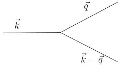
Figure 4: Self-decay of quantum fluctuations of the inflaton. All lines correspond to the field $\phi$, i.e, the quantum fluctuations of the inflaton.

Superhorizon modes: $k=0$

For superhorizon modes the results Eqs.(54) and (55) show that the amplitude of the quantum fluctuations decay as $\eta\rightarrow 0$ with the power law given by Eq.(55) with $\beta_{+}=2+\epsilon_{V}-\eta_{V},\;\beta_{-}=-1+\eta_{V}-\epsilon_{V}$ and

$$\Gamma=\frac{8}{9}\left[\frac{g}{\pi\,H\,(\eta_{V}-\epsilon_{V})}\right]^{2}\left[1+\mathcal{O}(\epsilon_{V},\eta_{V})\right]\;.$$ (87)

The effective dimensionless coupling $g/H$ [see Eq.(71)] is related to the scale of inflation and the slow roll parameters:

$$\frac{g}{H}=\frac{V^{\prime\prime\prime}[\Phi_{0}]}{2\;H}\sim\frac{\xi_{V}}{\sqrt{2\;\epsilon_{V}}}\;\frac{3\;H}{2\;M_{Pl}}$$ (88)

To lowest order in slow roll the power spectrum of curvature perturbations $\triangle^{2}_{\mathcal{R}}$ is given by liddle

$$\triangle^{2}_{\mathcal{R}}=\frac{H^{2}}{8\;\pi^{2}\;M^{2}_{Pl}\;\epsilon_{V}}=\frac{1}{12\;\pi^{2}\;M^{6}_{Pl}}\frac{V^{3}}{V^{\prime 2}}\;.$$ (89)

This allows to relate the effective dimensionless coupling $g/H$ to quantities that are observable from CMB data:

$$\frac{g}{H}=3\;\pi\;\xi_{V}\left(\triangle^{2}_{\mathcal{R}}\right)^{\frac{1}{2}}\left[1+\mathcal{O}(\eta_{V},\epsilon_{V})\right]\;.$$ (90)

Then, we can write $\Gamma$ [Eq.(87)] completely in terms of slow roll parameters and the power spectrum of curvature perturbations,

$$\Gamma=\frac{8\;\xi^{2}_{V}\;\triangle^{2}_{\mathcal{R}}}{(\epsilon_{V}-\eta_{V})^{2}}\left[1+\mathcal{O}(\epsilon_{V},\eta_{V})\right]\;,$$ (91)

and in terms of the scalar index and the tensor/scalar rate we have using Eq. (86),

$$\Gamma=32\;\frac{\xi^{2}_{V}\;\triangle^{2}_{\mathcal{R}}}{(n_{S}-1+\frac{r}{4})^{2}}\left[1+\mathcal{O}(\epsilon_{V},\eta_{V})\right]\;.$$ (92)

Of particular importance is the behavior of the growing mode of the inflaton which gives the dominant term for $\eta\to 0$ after the wavelengths of the fluctuations cross the horizon. ¿From Eqs. (43), (55) and (84), it is given by

$$\eta^{\beta_{-}+\Gamma}=\frac{\eta^{\eta_{V}-\epsilon_{V}+\Gamma}}{\eta}\;.$$ (93)

We see that the decay constant $\Gamma$ acts as an anomalous scaling dimension for the growing mode of the superhorizon fluctuations of the inflaton. The decay rate $\Gamma$ slows down the growth of the dominant mode for $\eta\to 0$ and fastens the decrease of the subdominant modes.

Modes inside the Hubble radius during slow roll inflation $|k\eta|\gg 1$:

The decay law of the quantum fluctuations of the inflaton with wavelengths deep inside the Hubble radius $|k\eta|=k_{ph}(\eta)/H\gg 1$ is given by Eqs.(III.4) with

$$\Gamma(|k\eta|\gg 1)=\frac{g^{2}}{32\;\pi\;H^{2}}\;\frac{H}{k_{ph}(\eta)}\;\left[1+\frac{2\;H}{\pi\;k_{ph}(\eta)}\left(\frac{1}{\eta_{V}-\epsilon_{V}}+\ln\frac{k_{ph}(\eta)}{H}\right)\right]~{}~{},~{}~{}k_{ph}(\eta)=\frac{k}{C(\eta)}~{}~{},~{}~{}C(\eta)=-\frac{1+\epsilon_{V}}{H\;\eta}\;.$$ (94)

The term that is inversely proportional to the slow-roll parameters and the logarithm of $k_{ph}(\eta)/H$ are a consequence of the almost collinear emission of superhorizon quanta. This process corresponds to one of the decay lines in fig. 4 carrying small momentum with superhorizon wavelengths as explained in the previous section. This process is identified as the emission of bremsstrahlung radiation of superhorizon quanta.

Which of the terms in the bracket in Eq.(94) dominates depends not only on the numerical value of the slow roll parameters but also on how close the physical wave vector is to horizon crossing. For very short wavelength modes, namely

$$k_{ph}(\eta)\gg\frac{2\;H}{\eta_{V}-\epsilon_{V}}$$ (95)

the second term is negligible and the result is similar to the inflaton decaying into massless conformally coupled particles. This is of course due to the fact that in this kinematic region the modes in the internal propagators are simply plane waves with Bunch-Davies initial conditions. On the contrary, as $k_{ph}(\eta)$ approaches horizon crossing,

$$k_{ph}(\eta)\lesssim\frac{H}{\eta_{V}-\epsilon_{V}}\;,$$ (96)

the emission of ultrasoft collinear quanta, namely superhorizon bremsstrahlung radiation, becomes the dominant decay channel and the second term dominates. This crossover phenomenom can be interpreted as the phase space for collinear emission opening up near horizon crossing. This is because the phase space factor $1/k$ in eq. (133) is effectively $1/|k\eta|=H/k_{ph}(\eta)$ by dimensional reasons.

Thus, in slow roll, there is a wide region of physical momenta

$$H\ll k_{ph}(\eta)\ll\frac{H}{\eta_{V}-\epsilon_{V}}\;,$$ (97)

for which the first term in the bracket in Eq.(94) can be neglected and the leading slow-roll result Eq.(90) for $g^{2}/H^{2}$ can be used:

$$\Gamma(|k\eta|\gg 1)=\frac{9}{16}\;\left(\frac{\xi_{V}\;\triangle_{\mathcal{R}}}{k\,\eta}\right)^{2}(1+2\,\epsilon_{V})\left\{\frac{1}{\eta_{V}-\epsilon_{V}}+\log[k\,\eta(1-\epsilon_{V})]\right\}\;.$$ (98)

V Implications for the decay of scalar and tensor perturbations and non-gaussianity

While we have focused on the decay of the inflaton quantum fluctuations during slow roll we can extrapolate our results to see how our findings may provide corrections to the power spectra of scalar and tensor perturbations.

V.1 Curvature perturbations:

For scalar perturbations, the action for the gauge invariant perturbation

$$u_{k}=C(\eta)\;\phi_{k}+\frac{\Phi^{\prime}_{0}}{H}\;\psi_{k}\;,$$ (99)

has a simple form at quadratic order bran and obeys the equation of motion

$$u^{\prime\prime}_{k}+\left[k^{2}-\frac{z^{\prime\prime}}{z}\right]u_{k}=0~{}~{};~{}~{}z\equiv\frac{\Phi^{\prime}_{0}}{H}\;.$$ (100)

Here $\Phi_{0}$ is the inflaton expectation value, $\phi_{k}$ the inflaton fluctuation and $\psi_{k}$ are the spatial curvature perturbations. The gauge invariant perturbation $u_{k}$ is related to the curvature perturbation on comoving hypersurfaces $\mathcal{R}$ as lidsey ; liddle ; bran $u_{k}=-z\;\mathcal{R}_{k}$. Therefore, the power spectrum of the curvature perturbation $\triangle^{2}_{\mathcal{R}}$ is directly related to the corresponding spectrum of the gauge invariant perturbation $u_{k}$ lidsey ; liddle ; bran

$$\triangle^{2}_{\mathcal{R}}=\frac{k^{3}}{2\pi^{2}}\left|\frac{u_{k}}{z}\right|^{2}\;.$$ (101)

For superhorizon modes, $k^{2}\ll z^{\prime\prime}/z$, the only relevant contribution is the growing mode $u_{k}=A_{k}\;z$. Therefore, well after horizon crossing the power spectrum of the curvature perturbation is constant in time and given by

$$\triangle^{2}_{\mathcal{R}}=\frac{k^{3}}{2\pi^{2}}\left|A_{k}\right|^{2}\;.$$ (102)

During slow roll lidsey ; liddle

$$\frac{z^{\prime\prime}}{z}=2\;C^{2}(\eta)\;H^{2}\left[1+\epsilon_{V}-\frac{3}{2}\;\eta_{H}\right]=\frac{2}{\eta^{2}}\left[1+\frac{3}{2}(\eta_{V}+\epsilon_{V})+\mathcal{O}(\eta^{2}_{V},\epsilon^{2}_{V},\eta_{V}\epsilon_{V},\xi_{V})\right]\equiv\frac{\nu^{2}-\frac{1}{4}}{\eta^{2}}$$ (103)

where we used Eqs.(74) and (78) and which implies

$$\nu=\frac{3}{2}+\epsilon_{V}+\eta_{V}+\mathcal{O}(\eta^{2}_{V},\epsilon^{2}_{V},\eta_{V}\epsilon_{V},\xi_{V})$$ (104)

Therefore, the small parameter $\Delta$ for the gauge invariant perturbation is given by

$$\Delta=-\epsilon_{V}-\eta_{V}+\mathcal{O}(\eta^{2}_{V},\epsilon^{2}_{V},\eta_{V}\epsilon_{V},\xi_{V})$$ (105)

Without interactions among fluctuations (no decay of fluctuations), the growing mode for superhorizon wavelengths to lowest order in slow roll is given by

$$u_{k}(\eta)=A_{k}~{}\eta^{-(1+\epsilon_{V}+\eta_{V})}$$ (106)

When a cubic interaction for the perturbation $u_{k}(\eta)$ is introduced, the results of the previous sections imply that an anomalous scaling dimension, namely the decay rate $\Gamma$ will appear in Eq. (106), i. e.

$$u_{k}(\eta)=A_{k}~{}\eta^{-(1+\epsilon_{V}+\eta_{V}-\Gamma)}\;,$$

as in Eq. (93) for the inflaton fluctuations. Unless $z$ acquires the same anomalous dimensions, the amplitude of the power spectrum [Eq. (101)] will depend on time.

In order to study the decay of curvature perturbations the next step in this program is to obtain the cubic vertex for the variable $u$ and to compute the one-loop self energy. This will ensure the gauge invariance of the results. The gauge invariant formulation of ref.bran has to be extended to higher order of perturbations, as for example in ref.bart , or alternatively, we can work in a fixed gauge. The cubic interaction vertex for three scalars has been computed in ref.maldacena . In particular, the contribution to the self-energy from ghost loops must be included.

The computation of the self-energy corrections will follow the same lines presented in the previous sections with the extra feature of momentum dependent vertices and ghost-loops. The infrared behavior of the loops will be regulated by $\Delta$ given by Eq.(105).

In order to obtain corrections for the power spectrum of curvature perturbations, the secular terms arising from the equations of motion will have to be resummed by DRG for the whole range of physical momenta, until and beyond horizon crossing, and establish the behavior of the growing mode. At least two sources of corrections to the index of the power spectra may be expected:

i) from the amplitude of the growing mode $A_{k}$, which is obtained by matching the solutions deep within the Hubble radius and well after horizon crossing,

ii) from the anomalous scaling dimension of the growing mode, namely the decay rate $\Gamma$.

Furthermore, in order to extract the power spectrum, the corrections to the dynamics of the zero mode of the inflaton $\Phi_{0}$ from the coupling of the zero mode to the fluctuations must be obtained. This study will indicate whether the variable $z$ also acquires an anomalous dimension and if so, whether the ratio $u_{k}/z$ for the growing mode is time independent when the decay process is accounted for. This study is in progress.

V.2 Gravitational waves:

For tensor modes, i.e, gravitational waves the action at the quadratic level is simple bran and the field operators for the (gauge invariant) gravitational waves are expanded in terms of the mode functions $V_{k}$ which satisfy

$$V^{\prime\prime}_{k}+\left[k^{2}-\frac{C^{\prime\prime}}{C}\right]V_{k}=0\;,$$ (107)

where $\frac{C^{\prime\prime}}{C}$ in given by Eq. (82). We then have

$$\frac{C^{\prime\prime}}{C}=\frac{\nu^{2}-\frac{1}{4}}{\eta^{2}}+\mathrm{higher~{}orders~{}in~{}slow~{}roll}\;,$$ (108)

i. e. ,

$$\nu=\frac{3}{2}+\epsilon_{V}+\mathrm{higher~{}orders~{}in~{}slow~{}roll}\quad,\quad\Delta=-\epsilon_{V}+\mathrm{higher~{}orders~{}in~{}slow~{}roll}\;.$$

Thus, during quasi de Sitter slow roll, the mode functions for gravitational waves are Hankel functions with an index $\nu$ slightly different from $3/2$.

The three graviton vertex was computed in refs.IRcosmo ; maldacena . The Born scattering amplitude for three gravitons in a de Sitter space-time features both infrared as well as secular divergencesIRcosmo . These infrared divergences precisely arise because the mode functions for gravitons in de Sitter space-time are Hankel functions with index $\nu=3/2$. The remaining long time ($\eta\rightarrow 0$) divergences can be consider as secular terms akin to those found above.

During quasi de Sitter slow roll inflation, the parameter $\Delta$ can regulate the infrared divergences found in refs. IRcosmo ; dolgov , and the DRG implemented here will provide a resummation of the secular long time divergences found in refs.IRcosmo and dolgov .

While the three graviton scattering amplitude has been computed in the Born approximation, the full self-energy for gravitons has not yet been obtained. In order to understand the decay law for gravitons, the program presented in this article must be implemented. Such program for gravitons, as in the case of the scalar perturbations discussed above, may require including the contribution from ghost loops to the graviton self-energy. Clearly, carrying this program in either case is a task beyond the scope of this article.

V.3 Estimates of the cubic coupling and the decay rate from the WMAP data

In the slow roll approximation the slow-roll parameters themselves are slowly varying functions of time, in particular

$$\frac{\dot{\eta}_{V}}{H}=2\;\epsilon_{V}\;\eta_{V}-\sqrt{2\epsilon_{V}}\;\frac{2M_{Pl}}{3H}\;\frac{g}{H}+\mathcal{O}(g\;\epsilon_{V}^{3/2})\;.$$ (109)

The slow roll approximation entails that $\dot{\eta}_{V}/H\ll 1$ which in turn requires

$$\frac{g}{H}\ll\frac{3H}{2\sqrt{2\epsilon_{V}}\,M_{Pl}}\;.$$ (110)

WMAP gives the following value for $\triangle^{2}_{\mathcal{R}}$ peiris

$$\triangle^{2}_{\mathcal{R}}\simeq 2.2\times 10^{-9}$$ (111)

which when combined with Eq.(89) yields the following estimate on the scale of inflation

$$H\sim 10^{15}\;\sqrt{\epsilon_{V}}\;[\mathrm{Gev}]$$ (112)

The WMAP data on $d\,n_{s}/d\ln k$ peiris suggests that $\xi_{V}\simeq 0.028\pm 0.015$ which combined with Eq. (90) leads to the following estimate on the cubic coupling,

$$\frac{g}{H}\simeq 1.3\times 10^{-5}$$ (113)

which places the strength of the dimensionless coupling within the validity of the slow roll approximation and perturbation theory. These results in turn lead to the following estimate for the rate $\Gamma$ [Eq. (91)],

$$3\times 10^{-8}\gtrsim\Gamma\gtrsim 3.6\times 10^{-9}\;.$$ (114)

This gives in cosmic time for a typical value $H\simeq 10^{14}$GeV

$$10^{7}\;GeV\gtrsim\Gamma_{dS}=H\;\Gamma\gtrsim 10^{6}\;GeV\;.$$ (115)

V.4 Connection with non-gaussianity:

Non-gaussianity of the spectrum of fluctuations is associated with three (and higher) point correlation functions. An early assessment of non-gaussian features of temperature fluctuations in an interacting field theory was given in ref.allen . In ref.srednicki the simplest inflationary potential with a cubic self-interaction for the inflaton field was proposed as a prototype theory to study possible departures from gaussianity. The three point correlation function of a scalar field in a theory with cubic interaction as well as the four point correlation function in a theory with quartic interaction were calculated in ref.uzan ; bartolo .

The long time ($\eta\rightarrow 0$) behavior of the equal time three point correlation function in the scalar field theory defined by Eq.(5) for $M=0$ (and hence $\nu=\frac{3}{2}$), is given by srednicki

$$\langle\chi(\vec{k},\eta)\;\chi(\vec{q},\eta)\;\chi(-\vec{k}-\vec{q},\eta)\rangle=\frac{2\pi^{3}}{3}\;C^{3}(\eta)\;g\;H^{2}\frac{F(\vec{k},\vec{q};\eta)}{\left[k\;q\;|\vec{k}+\vec{q}|\right]^{3}}$$ (116)

where

$$F(\vec{k},\vec{q};\eta)=\left[k^{3}+q^{3}+|\vec{k}+\vec{q}|^{3}\right]\left[\ln(k_{T}\eta)+\gamma\right]-(k^{2}+q^{2}+|\vec{k}+\vec{q}|^{2})k_{T}+k\,q\,|\vec{k}+\vec{q}|~{}~{};~{}~{}k_{T}=k+q+|\vec{k}+\vec{q}|$$ (117)

A diagrammatic interpretation of the equal time expectation value Eq.(116) is depicted in fig. 5, which illustrates the similarity with the decay process depicted in fig. 4.

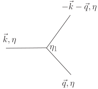
Figure 5: Equal time three point function $\langle\chi(\vec{k},\eta)\;\chi(\vec{q},\eta)\;\chi(-\vec{k}-\vec{q},\eta)\rangle$ in the Born approximation. The time coordinate $\eta_{1}$ of the vertex is integrated.

Furthermore, the logarithmic secular term in Eq.(117) indicates that the three point function features secular divergences even at the tree level. It is argued in refs. srednicki ; uzan ; bartolo that $-\ln[k_{T}\eta]\sim 60$ which is the number of e-folds from the time when fluctuations of wavenumber $k_{T}$ first crossed the horizon till the end of inflation. However, such infrared logarithms are secular terms and have precisely the same origin as in the self-energy kernel and in the inflaton fluctuations discussed here (secs. IIIC and IIID). The same holds for the infrared logarithms in the three graviton scattering vertex IRcosmo ; dolgov .

In particular, the self-energy computation corresponds to a further integration over the loop momentum $q$. In a fairly loose manner, the self-energy is basically the square of the three point correlation function integrated over the loop momentum. This is akin to the unitarity relation between the imaginary part of the forward scattering amplitude and the square of the transition amplitude in S-matrix theory.

In summary, the interaction between the fluctuations gives rise to non-gaussian correlations which are determined by the three point function which is precisely related to the self-energy and the decay of the quantum fluctuations. Therefore, the decay of the quantum fluctuations of the scalar field will also lead to non-gaussian correlations and non-gaussianity in the power spectrum.

The direct relationship between the self-energy, decay and non-gaussian features of the power spectrum will be the subject of further study.

VI Conclusions and further questions

In this article we have studied particle decay of fields minimally coupled to gravity in the case when the mass of the fields is $\ll H$ during inflation. Unlike the decay into massless fields conformally coupled to gravity, this case features a strong infrared behavior which leads to novel results.

We have implemented the dynamical renormalization group resummation program introduced in ref.desiterI combined with an expansion in a small parameter $\Delta$ which regulates the infrared.

In the case of exact de Sitter inflation, $\Delta$ is a constant equal to the ratio of the mass of the decay products to the Hubble constant, while in slow roll inflation $\Delta$ is a simple function of slow roll parameters. The expansion in $\Delta$ is akin to the $\varepsilon$ expansion in critical phenomena in dimensional regularization. The dynamical renormalization group provides a resummation of the long-time secular divergences which determine the decay law of quantum fluctuations.

The lack of energy conservation in an expanding cosmology leads to the lack of kinematic thresholds for particle decay. In particular, this possibility leads to the self-decay of quantum fluctuations whenever a self-interaction is present.

We have studied the decay of a particle for a cubic selfcoupled scalar field in de Sitter space-time and applied the results to the self-decay of the inflaton quantum fluctuations during quasi de Sitter, slow roll inflation. We focused on extracting the decay law both for wavelengths well inside and well outside the Hubble radius. In both cases the strong infrared behavior enhances the decay.

The decay of fluctuations with wavelengths much smaller than the Hubble radius is enhanced by the collinear emission of ultrasoft quanta, this process is identified as bremsstrahlung radiation of superhorizon quanta. As the physical wavelength approaches the horizon, the phase space for this process opens up becoming the dominant decay channel for short wavelength modes in the region

$$H\ll k_{ph}(\eta)\lesssim\frac{H}{\eta_{V}-\epsilon_{V}}\;.$$ (118)

The decay of short wavelength modes hastens as the physical wavelength approaches the horizon as a consequence of the opening up of the phase space.

Superhorizon quantum fluctuations decay as a power law $\sim\eta^{\Gamma}$ in conformal time, where $\Gamma$ is determined by the following combination of the slow roll parameters and the amplitude of curvature perturbations

$$\Gamma=\frac{32\;\xi^{2}_{V}\;\triangle^{2}_{\mathcal{R}}}{(n_{s}-1+\frac{r}{4})^{2}}\left[1+\mathcal{O}(\epsilon_{V},\eta_{V})\right]$$ (119)

This decay law entails that the growing mode for superhorizon wavelengths evolves as ${\eta^{\eta_{V}-\epsilon_{V}+\Gamma}}/{\eta}$ hence $\Gamma$ provides an anomalous scaling dimension slowing down the growing mode for $\eta\to 0$.

The recent WMAP data indicate that $3.\times 10^{-8}\gtrsim\Gamma\gtrsim 3.6\times 10^{-9}$. This corresponds to a decay rate in cosmic time $10^{7}GeV\gtrsim\Gamma_{dS}\equiv H\;\Gamma\gtrsim 10^{6}$GeV. Although these values may seem small, it must be noticed that the decay is a secular, namely cumulative effect.

We discussed some potential applications and implications for primordial scalar and tensor perturbations as well as the relationship between the decay processes studied in this article and the generation of non-gaussian features in the primordial power spectrum.

The results of our study bring about several questions:

• The generation of superhorizon fluctuations during inflation is usually referred to as ‘acausal’. However, we have found that fluctuation modes deep inside the horizon decay into superhorizon modes, therefore there is a coupling between modes inside and outside the horizon. The phase space for this process opens up as the physical wavelength approaches the horizon. It is natural to conjecture that this process that couples modes inside and outside the horizon with a coupling that effectively depends on the wave vector, will ultimately lead to distortions in the power spectrum. This distortion will necessarily be small in slow-roll since the coupling is of the order of the slow roll parameters, but it may compete with the running of the spectral index from the non-interacting theory which is itself of quadratic order in slow roll.

• In the non-interacting theory, the equation of motion for the gauge invariant Newtonian potential (equal to curvature perturbation) features a constant of motion for superhorizon wavelengths bardeen ; bran . This is used to estimate the spectrum of density perturbations in inflationary universe models. It is conceivable that this conservation law will no longer hold in higher order in slow roll when interactions are included. We expect this to be the case for two reasons: the coupling between modes inside and outside the horizon as well as the decay of superhorizon modes. Clearly the violation of the conservation law, if present, will be small in slow-roll, but this non-conservation may also lead to distortions in the power spectrum.

• While we have focused on the decay process during inflation, our results, in particular the decay of superhorizon fluctuations and the coupling between modes inside and outside the Hubble radius, raise the possibility of similar processes being available during the radiation dominated phase. If this is the case, the decay of short wavelength modes into superhorizon modes can serve as an active process for seeding superhorizon fluctuations.

Forthcoming observations of CMB anisotropies as well as large scale surveys with ever greater precision will provide a substantial body of high precision observational data which may hint at corrections to the generic and robust predictions of inflation. If such is the case these observations will pave the way for a better determination of inflationary scenarios. Studying the possible observational consequences of the quantum phenomena found in this article will therefore prove a worthwhile endeavor.

Appendix A Self-energy kernel for $\vec{k}=0$

We compute here the kernel $\mathcal{K}_{\bar{\nu}}(0,\eta,\eta^{\prime})$

$$\mathcal{K}_{\bar{\nu}}(0;\eta,\eta^{\prime})=\frac{1}{\pi^{2}}\int_{0}^{\infty}q^{2}\;dq~{}\mathrm{Im}\left\{\left[S_{\bar{\nu}}(q,\eta)S^{*}_{\bar{\nu}}(q,\eta^{\prime})\right]^{2}\right\}\quad,\quad\bar{\nu}=\frac{3}{2}-\Delta\;.$$ (120)

The infrared divergences at $\Delta=\frac{3}{2}-\bar{\nu}=0$ arise from the small momenta behavior of the integrand in Eq.(120). To extract such behavior it is convenient to write the Hankel function $H^{(2)}_{\bar{\nu}}(q\eta)$ in Eq. (15) as grad

$$H^{(2)}_{\bar{\nu}}(z)=\frac{i}{\sin\pi\bar{\nu}}\left[J_{-\bar{\nu}}(z)-e^{i\;\pi\;\bar{\nu}}\;J_{\bar{\nu}}(z)\right]\;.$$ (121)

The leading $q\to 0$ behavior follows from the Bessel functions $J_{-\bar{\nu}}(z)$ since grad ,

$$J_{-\bar{\nu}}(z)\buildrel z\to 0\over{=}\left(\frac{2}{z}\right)^{\bar{\nu}}\;\frac{1}{\Gamma(1-\bar{\nu})}\left[1+\mathcal{O}(z^{2})\right]\;.$$

We find upon taking the imaginary part,

$$\frac{q^{2}}{\pi^{2}}\mathrm{Im}\left\{\left[S_{\bar{\nu}}(q,\eta)\;S^{*}_{\bar{\nu}}(q,\eta^{\prime})\right]^{2}\right\}\buildrel q\to 0\over{=}-\left(\frac{4}{q^{2}\;\eta\,\eta^{\prime}}\right)^{\bar{\nu}-1}\;\frac{\Gamma^{2}(\bar{\nu})}{2\;\pi^{3}\;\bar{\nu}}\left[\left(\frac{\eta}{\eta^{\prime}}\right)^{\bar{\nu}}-\left(\frac{\eta^{\prime}}{\eta}\right)^{\bar{\nu}}\right]\left[1+\mathcal{O}(q^{2})\right]\;.$$ (122)

The behaviour $q^{2-2\,\bar{\nu}}=q^{2\,\Delta-1}$ for $q\to 0$ in the integrand of Eq. (120) implies a simple pole at $\Delta=0$ with a $\eta$-independent residue gel . It is then convenient to add and to subtract from Eq. (120) the low $q$ behaviour Eq. (122). We find,

$$\mathcal{K}_{\bar{\nu}}(0;\eta,\eta^{\prime})=I_{1}(\eta,\eta^{\prime};\mu)+I_{2}(\eta,\eta^{\prime};\mu)$$ (123)

with the integrals $I_{1,2}$ given by

$$I_{1}(\eta,\eta^{\prime};\mu)=\int_{0}^{\mu}dq\left(\frac{q^{2}}{\pi^{2}}\mathrm{Im}\left\{\left[S_{\bar{\nu}}(q,\eta)\;S^{*}_{\bar{\nu}}(q,\eta^{\prime})\right]^{2}\right\}+\left(\frac{2}{q^{2}\;\eta\,\eta^{\prime}}\right)^{\bar{\nu}-1}\;\frac{\Gamma^{3}(\bar{\nu})}{2\;\pi^{3}\;\Gamma(1+\bar{\nu})}\left[\left(\frac{\eta}{\eta^{\prime}}\right)^{\bar{\nu}}-\left(\frac{\eta^{\prime}}{\eta}\right)^{\bar{\nu}}\right]\right)$$ (124)

(125)

$$-\left(\frac{2}{\eta\,\eta^{\prime}}\right)^{\bar{\nu}-1}\;\frac{\Gamma^{3}(\bar{\nu})}{2\;\pi^{3}\;\Gamma(1+\bar{\nu})}\left[\left(\frac{\eta}{\eta^{\prime}}\right)^{\bar{\nu}}-\left(\frac{\eta^{\prime}}{\eta}\right)^{\bar{\nu}}\right]\int_{0}^{\mu}dq\;q^{2-2\,\bar{\nu}}\;,$$ (126)

$$I_{2}(\eta,\eta^{\prime};\mu)=\frac{1}{\pi^{2}}\int_{\mu}^{\infty}q^{2}\;dq~{}\mathrm{Im}\left\{\left[S_{\bar{\nu}}(q,\eta)S^{*}_{\bar{\nu}}(q,\eta^{\prime})\right]^{2}\right\}\;.$$ (127)

Here, $\mu>0$ is an arbitrary parameter temporarily introduced to split the integrals. The sum $I_{1}(\eta,\eta^{\prime};\mu)+I_{2}(\eta,\eta^{\prime};\mu)$ is clearly $\mu$-independent. The second integral in $I_{1}(\eta,\eta^{\prime};\mu)$ [Eq. (126)] can be done straightforwardly,

$$\int_{0}^{\mu}q^{2-2\bar{\nu}}\;dq=\frac{\mu^{2\;\Delta}}{2\;\Delta}\,.$$ (128)

This simple integral clearly displays the infrared divergence and the origin of the pole in $\Delta$: the emission of superhorizon quanta for which $q\eta,q\eta^{\prime}\ll 1$ as depicted in fig. 2.

Keeping the pole in $\Delta$ plus the leading logarithmic terms, and neglecting higher order terms in $\Delta$, we find for $\mu\eta,\mu\eta^{\prime}\ll 1$

$$I_{1}(\eta,\eta^{\prime};\mu)=\frac{1}{6\pi^{2}}\frac{1}{2\Delta}\left[\frac{\eta^{\prime}}{\eta^{2}}-\frac{\eta}{\eta^{{}^{\prime}2}}\right]+\frac{1}{6\pi^{2}}\left[\frac{\eta^{\prime}}{\eta^{2}}\ln[-\mu\eta]-\frac{\eta}{\eta^{{}^{\prime}2}}\ln[-\mu\eta^{\prime}]\right]+\mathcal{O}(\Delta)$$ (129)

We can set $3/2-\bar{\nu}=\Delta=0$ in the integral $I_{2}$ since it is infrared finite. After lengthy but straightforward algebra, we find for $\mu\eta,\mu\eta^{\prime}\ll 1$

$$I_{2}(\eta,\eta^{\prime};\mu)=-\frac{1}{8\pi^{2}}\mathcal{P}\left(\frac{1}{\eta-\eta^{\prime}}\right)+\frac{1}{6\pi^{2}}\Bigg{\{}\left(\frac{\eta}{\eta^{{}^{\prime}2}}-\frac{\eta^{\prime}}{\eta^{2}}\right)\left[\ln[\mu(\eta-\eta^{\prime})]+\gamma+\frac{5}{3}\right]+\left(\frac{1}{\eta^{\prime}}-\frac{1}{\eta}\right)\Bigg{\}}$$ (130)

the principal value P is defined by Eq. (47). The first term in Eq.(130) is the kernel for a massless conformally coupled field ($\bar{\nu}=1/2$)desiterI . It is clear from Eqs. (129) and (130) that the $\mu$ dependence cancels out as it should be:

$$\mathcal{K}_{\bar{\nu}}(0;\eta,\eta^{\prime})=\mathcal{K}_{\frac{1}{2}}(0;\eta,\eta^{\prime})+\frac{1}{6\pi^{2}}\Bigg{\{}\left[\frac{1}{2\Delta}+\frac{2}{3}\right]\left(\frac{\eta^{\prime}}{\eta^{2}}-\frac{\eta}{\eta^{{}^{\prime}2}}\right)-\frac{\eta^{\prime}}{\eta^{2}}\ln\left(\frac{\eta^{\prime}}{\eta}\right)+\left(\frac{\eta}{\eta^{{}^{\prime}2}}-\frac{\eta^{\prime}}{\eta^{2}}\right)\ln\left[1-\frac{\eta}{\eta^{\prime}}\right]+\frac{1}{\eta^{\prime}}-\frac{1}{\eta}\Bigg{\}}$$ (131)

where $\mathcal{K}_{\frac{1}{2}}(0;\eta,\eta^{\prime})$ is defined by Eq. (47).

Appendix B Self-energy kernel for $\vec{k}\neq 0$

The self-energy kernel $\mathcal{K}_{\bar{\nu}}(k;\eta,\eta^{\prime})$ for the general case is given by Eq.(23). As highlighted in the case of $\vec{k}=0$, there are infrared divergences for $\bar{\nu}=3/2$ which we regulated with the parameter $\Delta=3/2-\bar{\nu}$. We now compute $\mathcal{K}_{\bar{\nu}}(k;\eta,\eta^{\prime})$ keeping poles in $\Delta$ and the leading logarithms in $\eta$. The strategy is to separate the regions in the loop integral that contain the infrared divergences. Thanks to the azimuthal invariance we can write

$$\int d^{3}q=2\pi\int_{0}^{\infty}q^{2}~{}dq\int^{+1}_{-1}d(\cos\theta)$$ (132)

with $\theta$ the angle between $\vec{q}$ and $\vec{k}$. Furthermore, we change from the integration variable $\theta$ to $p=|\vec{q}-\vec{k}|$,

$$p=\sqrt{q^{2}+k^{2}-2\,k\,q\,\cos\theta}\quad,\quad d(\cos\theta)=\frac{dp}{k\;q}\;,$$ (133)

which clearly displays the phase space factor $1/k$. Eq.(23) takes then the symmetric form

$$\mathcal{K}_{\bar{\nu}}(k;\eta,\eta^{\prime})=\frac{\eta\,\eta^{\prime}}{32\,k}\int_{0}^{\infty}q\;dq\int_{|q-k|}^{q+k}p\;dp\;\mathrm{Im}\left[H^{(2)}_{\bar{\nu}}(q\eta)\;H^{(1)}_{\bar{\nu}}(q\eta^{\prime})\;H^{(2)}_{\bar{\nu}}(p\eta)\;H^{(1)}_{\bar{\nu}}(p\eta^{\prime})\right]\;.$$ (134)

where we used Eq. (15). The integral over $p$ can be performed using grad

$$\int p\;H^{(2)}_{\bar{\nu}}(p\eta)\;H^{(1)}_{\bar{\nu}}(p\eta^{\prime})\,dp=F_{\bar{\nu}}(p,\eta,\eta^{\prime})\;,$$ (135)

where,

$$F_{\bar{\nu}}(p,\eta,\eta^{\prime})=\frac{p}{\eta^{2}-\eta^{\prime 2}}\;\left[\eta^{\prime}\;H^{(2)}_{\bar{\nu}}(p\eta)\;H^{(1)}_{\bar{\nu}-1}(p\eta^{\prime})-\eta\;H^{(2)}_{\bar{\nu}-1}(p\eta)\;H^{(1)}_{\bar{\nu}}(p\eta^{\prime})\right]\;.$$ (136)

We obtain thus for the kernel,

$$\mathcal{K}_{\bar{\nu}}(k;\eta,\eta^{\prime})=\frac{\eta\,\eta^{\prime}}{32\,k}\;\mathrm{Im}\int_{0}^{\infty}q\;dq\left[F_{\bar{\nu}}(q+k,\eta,\eta^{\prime})-F_{\bar{\nu}}(|q-k|,\eta,\eta^{\prime})\right]H^{(2)}_{\bar{\nu}}(q\eta)\;H^{(1)}_{\bar{\nu}}(q\eta^{\prime})\;.$$ (137)

The infrared divergences at $\Delta=\frac{3}{2}-\bar{\nu}=0$ arise from the $q\to 0$ and $q\to k$ behavior of the integrand in Eq.(137). To extract such divergences we use the small argument behavior of the Hankel functions grad

$$H^{(2)}_{\bar{\nu}}(q\eta)\;H^{(1)}_{\bar{\nu}}(q\eta^{\prime})\buildrel q\to 0\over{=}\frac{\Gamma^{2}(\bar{\nu})}{\pi^{2}}\;\left(\frac{4}{q^{2}\;\eta\,\eta^{\prime}}\right)^{\bar{\nu}}\left[1+\mathcal{O}(q^{2})\right]\;,$$ (138)

(139)

$$F_{\bar{\nu}}(q,\eta,\eta^{\prime})\buildrel q\to 0\over{=}-\frac{\Gamma(\bar{\nu})\;\Gamma(\bar{\nu}-1)}{2\;\pi^{2}}\;\left(\frac{4}{\eta\,\eta^{\prime}}\right)^{\bar{\nu}}\;q^{2-2\,\bar{\nu}}\left[1+\mathcal{O}(q^{2})\right]\;.$$ (140)

We see from Eqs.(137) and (138) that the integrand in Eq.(137) behaves as $q^{2-2\,\bar{\nu}}=q^{2\,\Delta-1}$ for $q\to 0$ and as $|q-k|^{2-2\,\bar{\nu}}=|q-k|^{2\,\Delta-1}$ for $q\to k$. Therefore, the kernel has a simple pole at $\Delta=0$ gel . It is then convenient to add and to subtract from Eq. (137) the behaviour for $q\to 0$ and $q\to k$ Eq. (138) as we did in the Appendix A for the $k=0$ case. We find,

$$\mathcal{K}_{\bar{\nu}}(k;\eta,\eta^{\prime})=\frac{\eta\,\eta^{\prime}}{32\,k}\;\mathrm{Im}\int_{0}^{\infty}dq\left\{q\;\left[F_{\bar{\nu}}(q+k,\eta,\eta^{\prime})-F_{\bar{\nu}}(|q-k|,\eta,\eta^{\prime})\right]H^{(2)}_{\bar{\nu}}(q\eta)\;H^{(1)}_{\bar{\nu}}(q\eta^{\prime})\right.$$ (141)

(142)

$$-\left.\frac{\Gamma(\bar{\nu})\;\Gamma(\bar{\nu}-1)}{2\,\pi^{2}}\;\left(\frac{4}{\eta\,\eta^{\prime}}\right)^{\bar{\nu}}\;k\;H^{(2)}_{\bar{\nu}}(k\eta)\;H^{(1)}_{\bar{\nu}}(k\eta^{\prime})\left[4\,(\bar{\nu}-1)\;\theta(\mu-q)\;q^{2-2\bar{\nu}}+\theta(k-q+\mu)\;\theta(q-k+\mu)\;|q-k|^{2-2\bar{\nu}}\right]\right\}$$ (143)

(144)

$$+\frac{\Gamma(\bar{\nu})\;\Gamma(\bar{\nu}-1)}{8\,\pi^{2}}\;(\bar{\nu}-\frac{1}{2})\;\frac{\mu^{3-2\bar{\nu}}}{\frac{3}{2}-\bar{\nu}}\;\left(\frac{4}{\eta\,\eta^{\prime}}\right)^{\bar{\nu}-1}\;k\;\mathrm{Im}\;H^{(2)}_{\bar{\nu}}(k\eta)\;H^{(1)}_{\bar{\nu}}(k\eta^{\prime})\;.$$ (145)

$\mu>0$ is an arbitrary parameter temporarily introduced as in Appendix A and we used that

$$F_{\bar{\nu}}(q+k,\eta,\eta^{\prime})-F_{\bar{\nu}}(|q-k|,\eta,\eta^{\prime})\buildrel q\to 0\over{=}2\,q\frac{\partial F_{\bar{\nu}}(k,\eta,\eta^{\prime})}{\partial k}=2\,q\,k\;H^{(2)}_{\bar{\nu}}(k\eta)\;H^{(1)}_{\bar{\nu}}(k\eta^{\prime})\;.$$

$\mathcal{K}_{\bar{\nu}}(k;\eta,\eta^{\prime})$ is clearly $\mu$-independent as one can easily check by computing the derivative with respect to $\mu$ of the r. h. s. of eq.(141). Notice that $\theta(\mu-q)$ is nonzero for $q<\mu$ while $\theta(k-q+\mu)\;\theta(q-k+\mu)$ does not vanishes for $k-\mu<q<k+\mu$. The pole at $\frac{3}{2}-\bar{\nu}=\Delta=0$ is explicit in the last term of Eq.(141) while the integral over $q$ is finite for $\bar{\nu}=\frac{3}{2}$ and $k\neq 0$.

This analysis for the self-energy kernel shows that all infrared singularites emerge from the regions $|q\eta|,|q\eta^{\prime}|\ll 1$ and $|p\eta|,|p\eta^{\prime}|\ll 1$ corresponding to the internal line in the loop which carries momentum $q$ or $p=|q-k|$ being superhorizon. Both regions give a similar contribution because they are equivalent upon re-routing of the loop momentum and Bose symmetry. Thus the conclusion of this analysis is that the leading contributions to the self-energy arise from the collinear emission of superhorizon quanta [since $\cos\theta=1$, see Eq. (133)].

The calculation of the integral for $\mathcal{A}_{\bar{\nu}}(k;\eta,\eta^{\prime})$ in Eq. (141) is straightforward albeit lengthy. These are facilitated by the expression of the Hankel functions $H^{(1,2)}_{\frac{3}{2}}(q\eta)$ in terms of elementary functions. Dropping contributions of the order $\Delta$ the kernel in Eq. (141) becomes for $\mu\ll k,\;|\mu\eta|,|\mu\eta^{\prime}|\ll 1$,

$$\mathcal{K}_{\bar{\nu}}(k;\eta,\eta^{\prime})=\mathcal{K}_{\bar{\nu}}^{<}(k;\eta,\eta^{\prime})+\mathcal{K}_{\bar{\nu}}^{>}(k;\eta,\eta^{\prime})$$ (146)

with

$$\mathcal{K}_{\bar{\nu}}^{<}(k;\eta,\eta^{\prime})=\frac{\Gamma(\bar{\nu})\;\Gamma(\bar{\nu}-1)}{8\,\pi^{2}}\;(\bar{\nu}-\frac{1}{2})\;\frac{\mu^{3-2\bar{\nu}}}{\frac{3}{2}-\bar{\nu}}\;\left(\frac{4}{\eta\,\eta^{\prime}}\right)^{\bar{\nu}-1}\;\mathrm{Im}\;H^{(2)}_{\bar{\nu}}(k\eta)\;H^{(1)}_{\bar{\nu}}(k\eta^{\prime})\buildrel\Delta\to 0\over{=}$$ (147)

(148)

$$=\frac{1}{4\,\pi^{2}\,k^{3}\,(\eta\,\eta^{\prime})^{2}}\left\{k(\eta-\eta^{\prime})\cos[k(\eta-\eta^{\prime})]-(1+k^{2}\,\eta\,\eta^{\prime})\sin[k(\eta-\eta^{\prime})]\right\}\times$$ (149)

(150)

$$\left[\frac{1}{\Delta}+2\gamma-3+\log\left(4\,\mu^{2}\,\eta\,\eta^{\prime}\right)+D(k\eta,k\eta^{\prime})\right]$$ (151)

where,

$$D(k\eta,k\eta^{\prime})\equiv\frac{\pi}{2}\,k^{3}\,(\eta\,\eta^{\prime})^{3/2}\;\mathrm{Im}\left[H^{(2)}_{3/2}(k\eta)\;\left.\frac{\partial H^{(1)}_{\nu}(k\eta)}{\partial\nu}\right|_{\nu=3/2}+H^{(1)}_{3/2}(k\eta^{\prime})\;\left.\frac{\partial H^{(2)}_{\nu}(k\eta)}{\partial\nu}\right|_{\nu=3/2}\right]$$

and

$$\mathcal{K}_{\bar{\nu}}^{>}(k;\eta,\eta^{\prime})\buildrel\Delta\to 0\over{=}\frac{\eta\,\eta^{\prime}}{32\,k}\;\mathrm{Im}\int_{0}^{\infty}dq\left\{q\;\left[F_{3/2}(q+k,\eta,\eta^{\prime})-F_{3/2}(|q-k|,\eta,\eta^{\prime})\right]H^{(2)}_{3/2}(q\eta)\;H^{(1)}_{3/2}(q\eta^{\prime})\right.$$ (152)

(153)

$$-\left.\frac{k}{2\,\pi\;\left(\eta\,\eta^{\prime}\right)^{3/2}}\;H^{(2)}_{3/2}(k\eta)\;H^{(1)}_{3/2}(k\eta^{\prime})\left[\frac{2}{q}\;\theta(\mu-q)+\theta(k-q+\mu)\;\theta(q-k+\mu)\;\frac{1}{|q-k|}\right]\right\}\;,$$ (154)

where,

$$F_{3/2}(q,\eta,\eta^{\prime})=\frac{2}{\pi\sqrt{\eta\,\eta^{\prime}}}\;e^{iq(\eta^{\prime}-\eta)}\left[\frac{i}{\eta-\eta^{\prime}}-\frac{1}{q\,\eta\,\eta^{\prime}}\right]\;.$$

and

$$H^{(2)}_{3/2}(k\eta)\;H^{(1)}_{3/2}(k\eta^{\prime})=\frac{2}{\pi\;k^{3}\;(\eta\,\eta^{\prime})^{3/2}}\;e^{ik(\eta^{\prime}-\eta)}\left[1+k^{2}\;\eta\,\eta^{\prime}+i\,k(\eta-\eta^{\prime})\right]\;.$$

The integral for the kernel takes then form,

$$\mathcal{K}_{3/2}^{>}(k;\eta,\eta^{\prime})=\frac{\mathrm{Im}}{8\,\pi^{2}\,k\;\eta\,\eta^{\prime}}\int_{0}^{\infty}\frac{dq}{q^{2}}\left(\left[q^{2}\;\eta\,\eta^{\prime}+i\,q\,(\eta-\eta^{\prime})+1\right]\times\right.$$ (155)

(156)

$$\left.\left\{\frac{i}{\eta-\eta^{\prime}}\left[e^{i(2\,q+k)(\eta^{\prime}-\eta)}-e^{i(q+|q-k|)(\eta^{\prime}-\eta)}\right]-\frac{1}{\eta\,\eta^{\prime}}\left[\frac{e^{i(2\,q+k)(\eta^{\prime}-\eta)}}{q+k}-\frac{e^{i(q+|q-k|)(\eta^{\prime}-\eta)}}{|q-k|}\right]\right\}\right.$$ (157)

(158)

$$\left.-\frac{e^{ik(\eta^{\prime}-\eta)}}{k^{2}\;\eta\,\eta^{\prime}}\left[k^{2}\;\eta\,\eta^{\prime}+i\,k\,(\eta-\eta^{\prime})+1\right]\left[\frac{2}{q}\;\theta(\mu-q)+\frac{1}{|q-k|}\;\theta(k-q+\mu)\;\theta(q-k+\mu)\right]\right)$$ (159)

The remaining calculations are straightforward but tedious. Integrating over $q$ in Eq.(155) yields for $\mu\ll k,\;|\mu\eta|,|\mu\eta^{\prime}|\ll 1$,

$$\mathcal{K}_{3/2}^{>}(k;\eta,\eta^{\prime})=-\frac{1}{8\pi^{2}}\mathcal{P}\frac{\cos\alpha}{\eta-\eta^{\prime}}+$$

$$+\frac{1}{4\,\pi^{2}\,k^{3}(\eta\,\eta^{\prime})^{2}}\left\{\left[(1+k^{2}\;\eta\,\eta^{\prime})\sin\alpha-\alpha\,\cos\alpha\right]\left[\mathrm{Ci}(2\,\alpha)-1+\gamma+\log\left(2\;\frac{\mu^{2}}{k^{2}}\;\alpha\right)\right]\right.$$ (160)

(161)

$$\left.+2\;\sin\alpha-\mathrm{Si}(2\,\alpha)\left[(1+k^{2}\;\eta\,\eta^{\prime})\cos\alpha+\alpha\,\sin\alpha\right]\right\}$$ (162)

where $\alpha\equiv k(\eta-\eta^{\prime})$ , Ci(z) and Si(z) are the cosine and sine integral functions respectively grad . The first term in Eq. (B) is the kernel for conformally coupled massless particles and the principal part prescription is given by Eq. (47).

Keeping consistently the leading order terms in $\Delta$, namely the pole plus finite parts, the dependence on $\mu$ cancels out as it should and we find for the kernel to leading order in $\Delta$

$$\mathcal{K}_{\bar{\nu}}(k;\eta,\eta^{\prime})\buildrel\bar{\nu}\to 3/2\over{=}-\frac{1}{8\pi^{2}}\mathcal{P}\frac{\cos\alpha}{\eta-\eta^{\prime}}+$$

$$+\frac{1}{4\,\pi^{2}\,k^{3}(\eta\,\eta^{\prime})^{2}}\left\{\left[\alpha\,\cos\alpha-(1+k^{2}\;\eta\,\eta^{\prime})\sin\alpha\right]\left[\frac{1}{\Delta}+\gamma-2+\log\frac{2\,k\,\eta\,\eta^{\prime}}{\eta-\eta^{\prime}}-\mathrm{Ci}(2\,\alpha)+D(k\eta,k\eta^{\prime})\right]\right.$$ (163)

(164)

$$\left.+2\;\sin\alpha-\left[(1+k^{2}\;\eta\,\eta^{\prime})\cos\alpha+\alpha\,\sin\alpha\right]\mathrm{Si}(2\,\alpha)\right\}+\mathcal{O}(\Delta)\;.$$ (165)

Long wavelength limit: $|k\eta|,|k\eta^{\prime}|\ll 1$

The behavior of the kernel Eq. (B) in the limit when the wave vector $k$ corresponds to superhorizon wavelengths easily follows from Eq.(B). We use

$$Ci[\alpha]\buildrel\alpha\to 0\over{=}\ln\alpha+\gamma+\mathcal{O}(\alpha^{2})\quad,\quad Si[\alpha]\buildrel\alpha\to 0\over{=}\alpha-\frac{\alpha^{3}}{18}+\mathcal{O}(\alpha^{5})$$

Gathering all of these results and keeping the lowest order contributions in the limit $|k\eta|,|k\eta^{\prime}|\ll 1$ we find Eq. (46) for the kernel in the long-wavelength limit.

Short wavelength limit: $|k\eta|,|k\eta^{\prime}|\gg 1$

In this limit the wave function $S_{\bar{\nu}}(k,\eta)$ is just like the Minkowski space time free field mode function for massless fields, namely

$$S_{\bar{\nu}}(k,\eta)=\frac{e^{-ik\eta}}{\sqrt{2k}}.$$ (166)

It is straightforward to obtain the limit $|k\eta|,|k\eta^{\prime}|\gg 1$ of the kernel from Eq. (B) In the short wavelength limit the kernel simplifies to

$$\mathcal{K}_{\bar{\nu}}(k,\eta,\eta^{\prime})\buildrel\bar{\nu}\to 3/2,\;k^{2}\eta\eta^{\prime}\gg 1\over{=}-\frac{1}{8\pi^{2}}\mathcal{P}\frac{\cos k(\eta-\eta^{\prime})}{\eta-\eta^{\prime}}-\frac{1}{4\,\pi^{2}\,k\,\eta\,\eta^{\prime}}\Bigg{\{}\sin k(\eta-\eta^{\prime})\left[\frac{1}{\Delta}+\tilde{\mathcal{C}}+\log\frac{k\,\eta\,\eta^{\prime}}{\eta-\eta^{\prime}}\right]+\frac{\pi}{2}\;\cos k(\eta-\eta^{\prime})\Bigg{\}}\;,$$ (167)

with the constant $\tilde{\mathcal{C}}$ given by $\tilde{\mathcal{C}}=\ln 2+\gamma-2$.

References

- (1) A. Guth, Phys. Rev. D23, 347 (1981); astro-ph/0404546 (2004).
- (2) A. Albrecht and P. J. Steinhardt, Phys. Rev. Lett. 48,1220 (1982).
- (3) A. D. Linde, Phys. Lett. B108, 389 (1982); Phys. Lett. B129,177 (1983).
- (4) E. W. Kolb and M. S. Turner, The Early Universe Addison Wesley, Redwood City, C.A. 1990.
- (5) P. Coles and F. Lucchin, Cosmology, John Wiley, Chichester, 1995.
- (6) A. R. Liddle and D. H. Lyth, Cosmological Inflation and Large Scale Structure, Cambridge University Press, 2000; Phys. Rept. 231, 1 (1993), and references therein.
- (7) V. F. Mukhanov and G. V. Chibisov, Soviet Phys. JETP Lett. 33, 532 (1981).
- (8) S. W. Hawking, Phys. Lett. B115, 295 (1982).
- (9) A. H. Guth and S. Y. Pi, Phys. Rev. Lett. 49, 1110 (1982).
- (10) A. A. Starobinsky, Phys. Lett. B117, 175 (1982).
- (11) J. M. Bardeen, P. J. Steinhardt and M. S. Turner, Phys. Rev. D28, 679 (1983).
- (12) V. F. Mukhanov, H. A. Feldman and R. H. Brandenberger, Phys. Rept. 215, 203 (1992).
- (13) E. Komatsu et.al. (WMAP collaboration), Astro. Phys. Jour. Supp. 148, 119 (2003).
- (14) D. N. Spergel et.al. (WMAP collaboration), Astro. Phys. Jour. Supp. 148, 175 (2003).
- (15) A. Kogut et.al. (WMAP collaboration) Astro. Phys. Jour. Supp. 148, 161 (2003).
- (16) H. V. Peiris et.al. (WMAP collaboration),Astro. Phys. Jour. Supp. 148, 213 (2003).
- (17) D. N. Spergel and M. Zaldarriaga, Phys. Rev. Lett. 79, 2180 (1997); M. Zaldarriaga and D. D. Harari, Phys. Rev. D52, 3276 (1995).
- (18) T. J. Allen, B. Grinstein and M. B. Wise, Phys. Lett. B197, 66 (1987).
- (19) T. Falk, R. Rangarajan and M. Srednicki, Astrophys. J. 403, L1 (1993); Phys. Rev. D46, 4232 (1992).
- (20) A. Gangui, F. Lucchin, S. Matarrese and S.Mollerach, Astrophys. J. 430, 447 (1994).
- (21) J. Maldacena, JHEP 0305 , 013 (2003).
- (22) F. Bernardeau, T. Brunier and J.-P. Uzan, Phys.Rev. D69, 063520 (2004); F. Bernardeau and J.-P. Uzan, Phys.Rev. D67, 121301 (2003).
- (23) N. Bartolo, E. Komatsu, S. Matarrese and A. Riotto, astro-ph/0406398 (2004); V. Acquaviva, N. Bartolo,S. Matarrese and A. Riotto, Nucl. Phys. B667, 119 (2003).
- (24) D. Boyanovsky, H. J. de Vega, in the Proceedings of the VIIth. Chalonge School, ‘Current Topics in Astrofundamental Physics’, p. 37-57, edited by N. G. Sanchez, Kluwer publishers, Series C, vol. 562, (2001), astro-ph/0006446. D. Boyanovsky, D. Cormier, H. J. de Vega, R. Holman, S. P. Kumar, Phys. Rev. D 57, 2166 (1998). D. Boyanovsky, H. J. de Vega, R. Holman, Phys. Rev. D 49, 2769 (1994). D. Boyanovsky, F. J. Cao and H. J. de Vega, Nucl. Phys. B 632, 121 (2002), F. J. Cao, H. J. de Vega, N. G. Sanchez, astro-ph/0406168, to appear in Phys. Rev. D.
- (25) K. Enqvist, A. Mazumdar, M. Postma, Phys. Rev. D67, 121303(R) (2003). S. Tsujikawa, Phys. Rev. D68, 083510 (2003). G. Dvali, A. Gruzinov, M. Zaldarriaga, Phys. Rev. D69, 023505 and 083505 (2004). S. Matarrese, A. Riotto, astro-ph/0306416. A. Mazumdar, M. Postma, astro-ph/0306509. F. Vernizzi, Phys. Rev. D69, 083526 (2004); R. Allahverdi, astro-ph/0403351.
- (26) A. Berera and R. O. Ramos, hep-ph/0406339 (2004). A. Berera, Phys. Rev. Lett. 75, 3218 (1995), Phys. Rev. D54, 2519 (1996).
- (27) D. Boyanovsky, H. J. de Vega, Phys. Rev. D70, 063508 (2004).
- (28) J. Lidsey, A. Liddle, E. Kolb, E. Copeland, T. Barreiro and M. Abney, Rev. of Mod. Phys. 69 373, (1997).
- (29) D. Boyanovsky, R. Holman and S. Prem Kumar, Phys. Rev. D56, 1958 (1997).
- (30) S. Naidu and R. Holman, hep-th/0409013.
- (31) R. P. Woodard, astro-ph/0310757.
- (32) D. Boyanovsky, H. J. de Vega, Ann. of Phys. 307, 335 (2003); D. Boyanovsky, H. J. de Vega, R. Holman and M. Simionato, Phys. Rev. D 60 065003 (1999); D. Boyanovsky, H. J. de Vega, S.-Y. Wang, Phys.Rev. D67, 065022 (2003); D. Boyanovsky, H. J. de Vega, D.-S. Lee, S.-Y. Wang, H.-L. Yu, Phys.Rev. D65 , 045014 (2002); S.-Y. Wang, D. Boyanovsky, H. J. de Vega, D.-S. Lee, Phys.Rev. D62 , 105026 (2000).
- (33) N. C. Tsamis and R. P. Woodard, Class. Quantum Grav. 11 2969, (1994); Ann. of Phys. (N.Y.) 238, 1 (1995).
- (34) A. D. Dolgov, M. B. Einhorn and V. I. Zakharov, Phys. Rev. D52, 717 (1995).
- (35) W. Hu, astro-ph/0402060.
- (36) E. D. Stewart, Phys. Rev. D65, 103508 (2002); E. D. Stewart and J.-O. Gong, Phys. Lett. B510, 1 (2001); J.-O. Gong and E. D. Stewart, Phys. Lett. B538, 213 (2002).
- (37) N. Bartolo, S. Matarrese and A. Riotto, arXiv:astro-ph/0407505.
- (38) I. S. Gradshteyn and I. M. Ryzhik, Table of Integrals, Series and Products Academic Press, N.Y. 1965.
- (39) I. M. Gelfand and G. E. Shilov, Generalized Functions, vol I, Academic Press, New York, 1964.