Evolution of self–gravitating magnetized disks. II- Interaction between MHD turbulence and gravitational instabilities

Abstract

We present 3D magnetohydrodynamic (MHD) numerical simulations of the evolution of self–gravitating and weakly magnetized disks with an adiabatic equation of state. Such disks are subject to the development of both the magnetorotational and gravitational instabilities, which transport angular momentum outward. As in previous studies, our hydrodynamical simulations show the growth of strong $m=2$ spiral structure. This spiral disturbance drives matter toward the central object and disappears when the Toomre parameter $Q$ has increased well above unity. When a weak magnetic field is present as well, the magnetorotational instability grows and leads to turbulence. In that case, the strength of the gravitational stress tensor is lowered by a factor of about 2 compared to the hydrodynamical run and oscillates periodically, reaching very small values at its minimum. We attribute this behavior to the presence of a second spiral mode with higher pattern speed than the one which dominates in the hydrodynamical simulations. It is apparently excited by the high frequency motions associated with MHD turbulence. The nonlinear coupling between these two spiral modes gives rise to a stress tensor that oscillates with a frequency which is a combination of the frequencies of each of the modes. This interaction between MHD turbulence and gravitational instabilities therefore results in a smaller mass accretion rate onto the central object.

1 Introduction

In systems such as the disks surrounding low mass protostars or active galactic nuclei, the simultaneous appearance of both gravitational and magnetic instabilities is expected. During the first stages of their evolution, for example, protoplanetary disks are expected to be rather massive because of strong infall from the parent molecular cloud. As the disk builds up in mass as a result of the collapse of an envelope, its surface mass density becomes large enough for gravitational instabilities to develop (e.g., Laughlin & Bodenheimer 1994). These disks are also believed to be sufficiently ionized, at least over some extended regions, to be coupled to a magnetic field (Gammie, 1996; Sano et al., 2000; Fromang et al., 2002).

By modeling the outer parts of disks around quasi-stellar objects (QSOs) as steady, viscous, geometrically thin, and optically thick, Goodman (2003) has argued that they are self-gravitating. More precisely, he predicts self–gravitational instabilities to develop beyond about $10^{-2}$ parsecs from the central object. In addition, it has been suggested by Menou & Quataert (2001) that self-gravitating regions of disks around QSOs are likely to be coupled to a magnetic field.

The stability of a thin, self-gravitating gas disk is controlled by the Toomre $Q$ parameter (Toomre, 1964):

$$Q=\frac{c_{s}\kappa}{\pi G\Sigma}\,,$$ (1)

where $c_{s}$ is the sound speed, $\kappa$ is the epicyclic frequency (see, e.g., Binney & Tremaine 1987), $\Sigma$ is the disk surface mass density and $G$ is the gravitational constant. Gaseous disks are unstable against axisymmetric perturbations when $Q\leq 1$, and against non-axisymmetric perturbations when $Q\raisebox{-3.44444pt}{$\buildrel\textstyle>\over{\sim}$}1$.

Since analytical predictions of the nonlinear evolution of gravitational instabilities are difficult, there have been a large number of numerical simulations of gravitationally unstable disks. Despite the rather daunting technical problems of combining three-dimensional (3D) hydrodynamic calculations with rapid and accurate Poisson equation solvers, significant progress have been made. To do so, the energetics must be treated crudely, with the focus squarely on purely dynamical behavior. Using this strategy, the above $Q$ criterion for instability has been confirmed (and shown to still be approximately valid for disks of finite thickness), and the properties of the unstable modes have been studied as a function of the disk parameters (Tohline & Hachisu, 1990; Woodward et al., 1994). Several authors have investigated the saturation properties of the instability, and have shown that it is capable of transporting significant amount of mass and angular momentum in a few orbital times (Papaloizou & Savonije, 1991; Laughlin & Bodenheimer, 1994; Pickett et al., 1996; Laughlin et al., 1997). The first calculations mostly used simple adiabatic equations of state (EOS). More recently, isothermal disks have also been studied (Pickett et al., 1998, 2000; Boss, 1998; Mayer et al., 2002). Some new investigations also include a simplified treatment of the disk radiative cooling (Pickett et al., 2003; Rice et al., 2003; Boss, 2002).

All these models were purely hydrodynamical, and neglected the effect of magnetic fields. However, it is known that stability of astrophysical disks is extremely sensitive to the presence of weak magnetic fields. In particular, the magnetorotational instability (MRI) completely disrupts laminar Keplerian flow when a subthermal magnetic field of any geometry is present. This was first understood by Balbus & Hawley (1991). Since then, it has been shown through many numerical simulations that the nonlinear outcome of the MRI is MHD turbulence, which, in common with gravitational instabilities, transports angular momentum outward (see Balbus & Hawley 1998, or Balbus 2003, for a review). Since disks around low–mass stars and around QSOs may be both magnetized and self–gravitating, the spiral structure gravitational transport described above must somehow develop in a medium in the throes of MHD turbulence.

The question naturally arises as to how these two powerful instabilities interact with one another. What is the ultimate effect on the global properties of accretion disks, and in particular, on the critical transport properties of mass and angular momentum? To keep this initial investigation tractable, we must restrict ourselves here to an adiabatic EOS. But the dynamical behavior of “simple” adiabatic disks is still rich, and contains unanticipated findings. In a companion paper to this one (Fromang et al. 2004, hereafter paper I), we carried out 2D axisymmetric numerical simulations of the evolution of massive and magnetized disks. The results show that the MRI behaves in a self–gravitating environment as it does in zero mass disks. Turbulent transport of angular momentum causes the disk to evolve toward a two component structure: (1) an inner thin disk in Keplerian rotation fed by (2) an outer thick disk whose rotation profile deviates from Keplerian, strongly influenced by self-gravity. However, angular momentum transport by gravitational instabilities cannot develop in axisymmetric simulations, which leaves unanswered the question of the outcome of the interaction between both instabilities. This is the subject of the present paper.

The plan of the paper is as follows: in section 2, we present our numerical methods. The initial state of our simulations will be described in section 3. We present our results in section 4 and, finally, give our conclusions in section 5.

2 Numerical methods

2.1 Algorithms

The calculations in this paper are based on the equations of ideal MHD:

$$\frac{\partial\rho}{\partial t}+\mbox{\boldmath{$\nabla$}}\mbox{\boldmath{$\cdot$}}(\rho{\bf v})=0,$$ (2)

$$\rho\left(\frac{\partial{\bf v}}{\partial t}+{\bf v}\mbox{\boldmath{$\cdot$}}\mbox{\boldmath{$\nabla$}}{\bf v}\right)=-\mbox{\boldmath{$\nabla$}}P-\rho\mbox{\boldmath{$\nabla$}}\Phi+\frac{1}{4\pi}(\mbox{\boldmath{$\nabla$}}\mbox{\boldmath{$\times$}}{\bf B})\mbox{\boldmath{$\times$}}{\bf B},$$ (3)

$$\rho\left(\frac{\partial}{\partial t}+{\bf v}\mbox{\boldmath{$\cdot$}}\mbox{\boldmath{$\nabla$}}\right)\left(\frac{e}{\rho}\right)=-P\mbox{\boldmath{$\nabla$}}\mbox{\boldmath{$\cdot$}}{\bf v},$$ (4)

$$\frac{\partial{\bf B}}{\partial t}=\mbox{\boldmath{$\nabla$}}\mbox{\boldmath{$\times$}}({\bf v}\mbox{\boldmath{$\times$}}{\bf B}),$$ (5)

where $\rho$ is the mass density, $e$ is the energy density, $\bf{v}$ is the fluid velocity, $\bf{B}$ is the magnetic field, $P$ is the gas pressure and $\Phi=\Phi_{s}+\Phi_{c}$ is the total gravitational potential, which has contributions $\Phi_{s}$ from the disk self–gravity and $\Phi_{c}$ from a central mass. The Poisson equation determines the gravitational potential,

$$\nabla^{2}\Phi_{s}=4\pi G\rho,$$ (6)

and to close our system of equations, we adopt an adiabatic equation of state for a monoatomic gas:

$$P=(\gamma-1)e,\quad\gamma=5/3.$$ (7)

To solve these equations, we use the GLOBAL code (Hawley & Stone, 1995). This uses standard cylindrical coordinates $(r,\phi,z)$ and time–explicit Eulerian finite differences. The magnetic field is evolved using the combined Method of Characteristics and Constrained Transport algorithm (MOC–CT), which preserves the divergence of the magnetic field to machine accuracy. Finally, we use outflow boundary conditions in the radial and vertical directions, and periodic boundary conditions in $\phi$.

In its original form, GLOBAL did not include a Poisson solver, and the development of such a routine represents a major technical component of the results we report here. The calculation is done in two steps. The potential $\Phi_{s}$ is first computed at the grid boundary, using the spectral decomposition decribed below, and then calculated on the whole grid using a very rapid method. It is the first step, the boundary calculation, that is computationally expensive.

In the expansion of $\Phi_{s}$, we have adopted the method of Cohl & Tohline (1999), which uses half–integer Legendre functions in the Green’s function. This method is better suited to cylindrical coordinates than the traditional expansion in spherical harmonics, which are of course tailored to spherical coordinates. Following Cohl & Tohline (1999), $\Phi_{s}$ may be written

$$\Phi_{s}(r,\phi,z)=-\frac{G}{\pi\sqrt{r}}\int_{V}d\tau^{\prime}\;\frac{\rho(r^{\prime},\phi^{\prime},z^{\prime})}{\sqrt{r^{\prime}}}\sum_{m=0}^{\infty}\epsilon_{m}Q_{m-1/2}(\chi)\cos m(\phi-\phi^{\prime})\;.$$ (8)

Here, $d\tau^{\prime}=r^{\prime}dr^{\prime}d\phi^{\prime}dz^{\prime}$ is the elementary volume element, and the integral is taken over the whole computational domain. $Q_{m-1/2}$ denotes the half–integer order Legendre function of the second type (Abramowitz & Stegun, 1965). The argument $\chi$ is a function of position:

$$\chi=\frac{r^{2}+r^{\prime 2}+(z-z^{\prime})^{2}}{2rr^{\prime}}\,.$$ (9)

The Legendre functions are computed once at the beginning of each simulation and stored in memory. At each time step, we calculate $\Phi_{s}$ using equation (8), in which the sum over $m$ is truncated at some upper value $m_{max}$. We then calculate $\Phi_{s}$ everywhere on the grid, using a combination of a Fourier transform in $\phi$ and the 2D Successive Over Relaxation (SOR) Method (Hirsch, 1988) in the $(r,z)$ plane. Although this is an efficient method, the calculation of the self–gravitating potential is still very demanding of computational resources. For the resolution $(N_{r},N_{\phi},N_{z})=(128,64,128)$ used in this paper, the time required by the Poisson solver still represents $\sim 40\%$ of the computation time for $m_{max}=8$.

2.2 Diagnostics

We introduce and define some key quantities that have been used to analyze the results of the simulations. We denote the ratio of the volume averaged thermal pressure to the volume averaged magnetic pressure as $\langle\beta\rangle$:

$$\langle\beta\rangle=\frac{\langle P\rangle}{\langle B^{2}/8\pi\rangle}\,.$$ (10)

This parameter is used primarily as a measure of the initial magnetic field strength.

In 3D numerical simulations of magnetized self–gravitating disks, angular momentum is transported by the sum of the Maxwell, Reynolds, and gravitational stress tensors. Following Balbus & Papaloizou (1999) and Hawley (2000), we define the height and azimuthal averages (noted with an overbar) of each these respective stresses as:

$$T^{Max}_{r\phi}(r,t) = -\frac{\overline{B_{r}B_{\phi}}}{4\pi}\,,$$ (11)

$$T^{Ren}_{r\phi}(r,t) = \overline{\rho v_{r}v_{\phi}}-\frac{\overline{\rho v_{r}}\textrm{ }\overline{\rho v_{\phi}}}{\overline{\rho}}\,,$$ (12)

$$T_{r\phi}^{grav}(r,t) = \frac{1}{4\pi G}\overline{\frac{\partial\Phi_{s}}{\partial r}\frac{1}{r}\frac{\partial\Phi_{s}}{\partial\theta}}\,.$$ (13)

As in paper I, volume averages of these quantities will be denoted as $\langle T^{Max}_{r\phi}\rangle(t)$, etc. Note that $T_{r\phi}^{grav}$ is associated with the gravitational torque resulting from non-axisymmetric disk structure. This quantity clear vanishes in an axisymmetric simulation ($m_{max}=0$). In this case, the standard $\alpha$ parameter (Shakura & Sunyaev, 1973) can be defined as the sum of the Maxwell and Reynolds stress tensors normalized by the gas pressure:

$$\alpha(r,t)=\frac{T^{Max}_{r\phi}(r,t)+T^{Ren}_{r\phi}(r,t)}{\overline{P(r,t)}}\,.$$ (14)

3 Initial model

We start our simulations with a disk model which is as close as possible to hydrostatic equilibrium:

$$-\mbox{\boldmath{$\nabla$}}P-\rho\mbox{\boldmath{$\nabla$}}\left(\Phi_{s}+\Phi_{c}\right)+\rho r\Omega^{2}{\mbox{\boldmath{$e$}}_{r}}={\bf 0}\,.$$ (15)

Here $\Omega$ is the angular velocity and $e_{r}$ is the unit vector in the radial direction. The coordinate system has its origin on the disk center. The potential $\Phi_{c}$ is due to a central mass $M_{c}$. We chose $M_{c}=2M_{d}$, where $M_{d}$ is the disk mass. The initial disk model is gravitationally unstable.

Because of the presence of the disk self–gravity, equation (15) has to be solved iteratively. We use the Self–Consistent Field (SCF) iterative method developed by Hachisu (1986). In this method, the radial profile of the angular velocity $\Omega$ or, equivalently, the specific angular momentum $j=r^{2}\Omega$, is specified. Following Pickett et al. (1996), we fix $j(r)$:

$$j=j_{r0}\left(\frac{M_{r}+M_{c}}{M_{d}+M_{c}}\right)^{q}$$ (16)

where $j_{r0}$ and $q$ are constant, and $M_{r}$ is the disk mass within radius $r$. Setting $q=2$ gives a $j$ profile close to that used by Pickett et al. (1996). We begin the iteration with an arbitrary mass density $\rho$, from which we can calculate $\Phi_{s}$. From $\rho$ and the above expression for $j$ we also calculate $\Omega$ (note that it still depends on the constant $j_{r0}$). The relation (15) is then integrated to give the value of the enthalpy $h$:

$$h=\frac{5}{2}K\rho^{2/3}=C-\left(\Phi_{s}+\Phi_{c}\right)+\int r\Omega^{2}dr\,,$$ (17)

where the constant $C$ and $j_{r0}$ are determined from the boundary conditions $\rho=0$ at $\left(r=R_{in},z=0\right)$ and at $\left(r=R_{out},z=0\right)$. Here $R_{in}$ and $R_{out}$ are the radial boundaries of the disk. The new density field is then calculated from $h$ using the normalizing condition that $\rho_{max}=1$, which determines the polytropic constant $K$. Upon iterating this procedure, we converge to a model very close to equilibrium.

The resulting disk model (with $R_{in}=0.25$ and $R_{out}=1$) has an $\Omega$ profile close to Keplerian and a density profile displayed in figure 1. Note that the disk is rather thin, with an aspect ratio $H/r$ varying between $0.1$ and $0.2$.

Figure 1: Density contours in the $(r,z)$–plane of the initial disk model used in all the simulations. The contours shown are $\rho=10^{-7},10^{-4},10^{-3},0.01,0.1,0.5,0.7$ and $0.9$. The disk radial boundaries are $R_{in}=0.25$ and $R_{out}=1$. The central mass is twice that of the disk.

As noted above, the ratio $M_{c}/M_{d}$ is chosen in such a way that the Toomre $Q$ parameter is initially close to unity. The radial profile of $Q$ in the initial disk model is shown in figure 2. The minimum value of $Q$ is approximately $1.1$, and $Q$ is close to unity over a large range of radii. We therefore expect strong non–axisymmetric gravitational instabilities to develop in this disk.

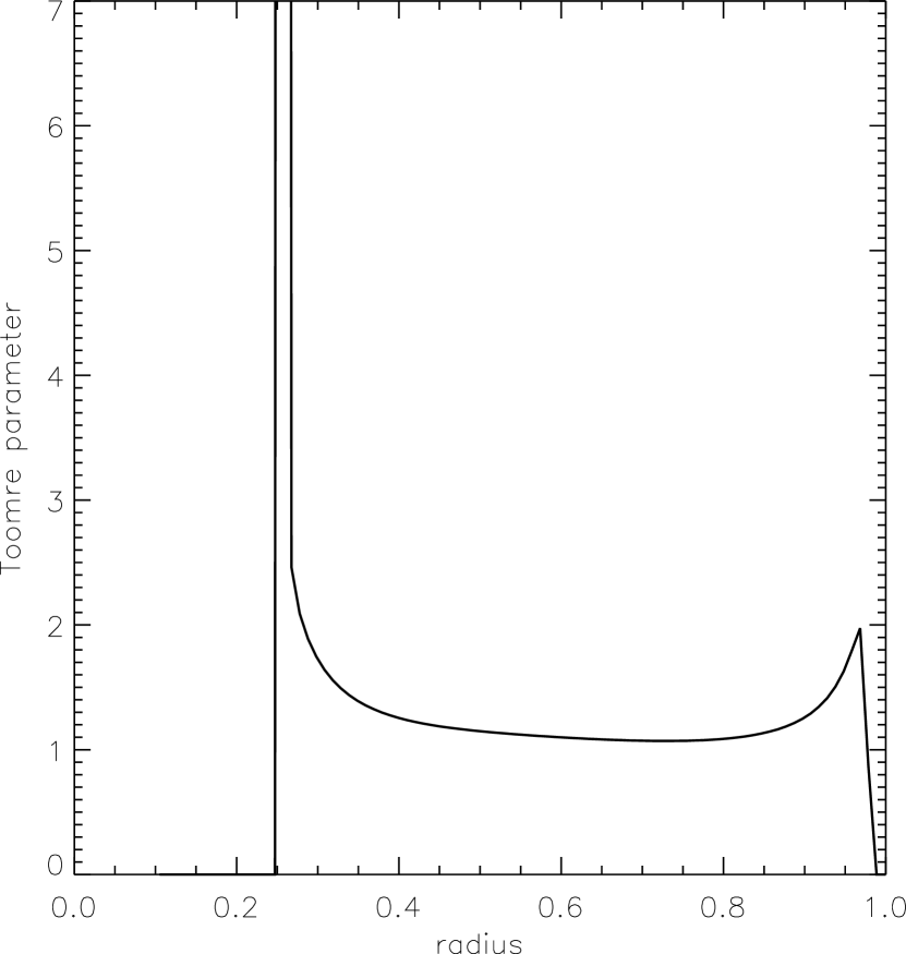
Figure 2: Radial profile of the Toomre $Q$ parameter in the initial disk model. $Q$ is close to unity over a large range of radii.

4 Results

Table 1 lists the parameters of the different runs we present below. Column $1$ gives the label of the model. HD refers to a hydrodynamical run. Models T and P start with a purely toroidal and poloidal magnetic field, respectively. Column 2 gives the computational azimuthal domain and column 3 gives the highest fourier component of the gravitational potential. When $m_{max}=0$, i.e. when only the $m=0$ component in the Fourier expansion of $\Phi_{s}$ is included, gravitational instabilities cannot develop (recall that $Q>1$, so that the disk is stable against axisymmetric perturbations). Therefore, models T1 and P1 enable us to study the evolution of MHD turbulence and to compare it with previous work and with the 2D simulations of paper I. In models T2, T2_low, T2^∗, T3 and P2, both gravitational and magnetic instabilities develop. In model T2^∗, the non–axisymmetric part of $\Phi_{s}$ is included only after $6$ orbits, i.e. after MHD turbulence has established itself. Column 4 gives the ratio of the volume-averaged thermal and magnetic pressures and column 5 gives the resolution $(N_{r},N_{\phi},N_{z})$ of the run.

Model	$\phi$–range	$m_{max}$	$\langle\beta\rangle$	Resolution
HD	$[0,\pi]$	$8$	$\infty$	$(128,64,64)$
T1	$[0,\pi/2]$	$0$	$8$	$(128,32,128)$
T2	$[0,\pi]$	$8$	$8$	$(128,64,128)$
T2low	$[0,\pi]$	$8$	$8$	$(64,64,64)$
T2∗	$[0,\pi]$	$0$–$8^{\dagger}$	$8$	$(128,64,128)$
T3	$[0,\pi]$	$16$	$8$	$(128,64,128)$
P1	$[0,\pi/2]$	$0$	$300$	$(128,32,128)$
P2	$[0,\pi]$	$8$	$300$	$(128,64,128)$

^† For this run, $m_{max}=0$ when $t\in[0,5.8]$, while $m_{max}=8$ for $t>5.8$.

Table 1: Model parameters. Column 2 gives the computational azimuthal domain, column 3 gives the highest Fourier component of the gravitational potential included in the calculation, column 4 gives the ratio of the volume averaged thermal and magnetic pressures and column 5 gives the resolution $(N_{r},N_{\phi},N_{z})$ of the run. Model HD is hydrodynamical. Models T and P start with a purely toroidal and poloidal magnetic field, respectively. When $m_{max}=0$, the disk self–gravitating potential is forced to stay axisymmetric. In model T2^∗, $m_{max}=0$ at the beginning of the run and is set to 8 after a few orbits.

In all the models, an adiabatic equation of state is used. The computational domain extends radially from 0.1 to 1.4, and vertically from $-0.2$ to $0.2$. In the azimuthal direction, the computational domain extends from 0 to either $\pi/2$ or $\pi$. The smaller range is used in the $m_{max}=0$ gravitationally stable cases. Indeed, Hawley (2000) and Papaloizou & Nelson (2003) have shown that an azimuthal domain of $\pi/3$ is generally sufficient to describe the transport properties of MHD turbulence. When we allow for the development of gravitational instabilities, we restrict the azimuthal domain to the half disk $[0,\pi]$. This saves computational time, but of course allows only even modes to develop. The focus of the paper is not on the detailed spectrum of modes which appear in a given disk model, however, but on the interaction between MHD turbulence and the largest scale gravitational modes. This interaction should not be particularly sensitive to whether an integer number of modes exactly fits in the half disk.

Time is measured in units of the orbital period at the initial outer edge $R_{out}=1$ of the disk model. Typical simulations are carried out for $8$ to $10$ orbits at this position. This corresponds to 60–80 orbits at the initial disk inner edge. The simulations are seeded by adding to the mass density at $r>0.4$ random perturbations with a relative amplitude of $5\times 10^{-3}$.

We now describe in turn the hydrodynamical run, the simulations with only MHD turbulence, and the runs with both gravitational and magnetic instabilities.

4.1 Control Hydrodynamical Run: Model HD

The time evolution of the Fourier components of the density in the equatorial plane is shown in figure 3 for the modes $m=2,4$ and $6$ (from top to bottom). The $m=2$ mode grows at the beginning of the simulation and saturates after $4$ orbits. Higher $m$ modes emerge after about $3$ orbits. Apart from the $m=4$ mode, which may also be linearly unstable, the $m>2$ modes appear to be non–linearly excited.

Figure 3: Time evolution of the Fourier components of the density in the equatorial plane for model HD. The $y$–axis represents the ratio of the amplitude of the $m$–th Fourier component of the perturbed density to the unperturbed density. From top to bottom, the different curves correspond to the modes $m=2$ (solid line), $m=4$ (dashed line) and $m=6$ (dotted-dashed line).

The development of a $m=2$ spiral structure may be seen in figure 4, which shows the logarithm of the density in the equatorial plane at $t=4.27$. (Note that the result of the simulation has been extended by symmetry to cover the range $[0,2\pi]$). This mode is clearly global. Its pattern speed is $\Omega_{p}=6.28$, which means that corotation (the radius where the gas angular velocity matches the pattern speed) is located at the initial outer edge of the disk. Such a mode is predicted to emerge by linear stability analyses of self-gravitating disks (Papaloizou & Savonije, 1991). The instability is due to the interaction between waves that propagate near the outer boundary and waves that reside inside the inner Lindblad resonance (where the pattern speed in the frame corotating with the planet matches the gas epicyclic frequency). This is located at $r\sim 0.6$ in our disk model.

Figure 4: Logarithm of the density in the equatorial plane for model HD at $t=4.27$. The linearly unstable two–arm global mode has become non–linear. It drives angular momentum outward and matter toward the central point mass.

During the simulation, matter is driven toward the disk center by the gravitational torque associated with the spiral arms and, at $t\simeq 8$, $Q$ has become sufficiently high ($\raisebox{-3.44444pt}{$\buildrel\textstyle>\over{\sim}$}2$) that the disk settles into a stable state. The results of this simulation are in agreement with theoretical expectations and with previous work, and show that the Poisson solver performs satisfactorily in the hydrodynamical regime.

4.2 MHD Simulations in an Axisymmetric Gravitational Potential

In the presence of a weak magnetic field, we expect our disk model to be unstable to the MRI, regardless of the field geometry. We first perform simulations in which only the MRI develops (models T1 and P1). This allows the properties of the ensuing MHD turbulence to be quantified and compared with previous work. To prevent the growth of non–axisymmetric gravitational instabilities, we retain only the $m=0$ component in the Fourier expansion of $\Phi_{s}$. The resolution is $(N_{r},N_{\phi},N_{z})=(128,32,128)$ and the azimuthal domain extends from 0 to $\pi/2$, which would be equivalent to a resolution of $128^{3}$ over a range of $2\pi$.

4.2.1 Initial toroidal field: Model T1

We add to the equilibrium disk model described above a $\langle\beta\rangle=8$ toroidal magnetic field and run the simulation for about $10$ orbits (about $80$ orbits at the initial disk inner edge).

Figure 5 shows the time evolution of the volume-averaged Maxwell and Reynolds stress tensors and the corresponding $\alpha$ parameter (see eq. [14]). The Maxwell stress increases during the linear phase of the instability. It then saturates after 4 orbits, when the MRI breaks down into turbulence. The presence of turbulence is seen in figure 6, which shows the density perturbation in the equatorial plane at $t=6.4$. Turbulent fluctuations are present over the full extent of the disk. It is clear from figure 5 that the Reynolds stress is significantly smaller than the Maxwell stress over the course of the simulation. This is in agreement with previous non self–gravitating global simulations of the MRI (Hawley, 2000, 2001; Steinacker & Papaloizou, 2002). The right panel of figure 5 shows the radial profile of $\alpha$ at the end of the simulation, i.e. at $t\simeq 10$. The typical value of $\alpha$ is a few times $10^{-2}$, similar to what was found in previous simulations starting with a toroidal field with a net flux (Steinacker & Papaloizou, 2002).

Figure 5: Left panel: Time evolution of the volume averaged Maxwell (solid line) and Reynolds (dashed line) stress tensors for model T1. The Maxwell stress increases during the linear growth of the MRI (first $4$ orbits). It then saturates when the instability breaks down into turbulence and stays roughly constant. At all time, the Reynolds stress is much smaller than its magnetic counterpart. Right panel: $\alpha$ vs. $r$ at the end of the simulation, i.e. at $t\simeq 10$. The typical value of $\alpha$ is a few times $10^{-2}$.

Figure 6: Density perturbation in the equatorial plane for run T1 at $t=6.4$. Turbulent fluctuations are present over the whole extent of the disk.

The Maxwell stress stays roughly constant during our simulation. This indicates that the resolution $(128,32,128)$ is large enough for the turbulence to be sustained over the duration of the run. We therefore adopt it in the following runs (which of necessity are limited in time by the fact that mass is accreted onto the central mass).

4.2.2 Initial poloidal field: Model P1

To investigate the sensitivity of our results to the initial field geometry, we run the same calculation as in model T1 but with an initial poloidal magnetic field. We calculate the field from the (toroidal) component of the vector potential in the initial disk model:

$$A_{\phi}\propto\rho\cos\left(8\pi\frac{r-R_{in}}{R_{out}-R_{in}}\right)\,.$$ (18)

This corresponds to 4 magnetic loops confined inside the disk. The first 2D simulations of a disk permeated by a weak vertical field (Hawley & Balbus, 1991) showed the development and growth of “channel” solutions. In 3D, these solutions still exist but they quickly break down into turbulence, as predicted by the analysis of Goodman & Xu (1994). Turbulence is more rapidly established when the field varies on a fairly small scale, which motivates the above choice of $A_{\phi}$.

The radial and vertical components of the magnetic field are computed from $A_{\phi}$ and normalized such as to obtain the desired initial value of $\langle\beta\rangle$. Since the linear growth of the vertical field is much more rapid than that of the toroidal field (see below), we chose a much larger initial value of $\langle\beta\rangle=300$.

The properties of the turbulence are similar to those found when the initial field is toroidal. Figure 7 shows the time evolution of the Maxwell stress for both models T1 and P1. As expected, the linear instability is much more vigorous when a vertical field is present, because of the growth of the channel solutions. However, in both cases the stress saturates at a similar value and the level of turbulence is comparable. The evolution of the Maxwell stress in P1 is somewhat similar to what was obtained in paper I. The important difference is that in 3D, the stress saturates when turbulence is established and does not decay with time, as it does in 2D.

Figure 7: Time history of the volume averaged Maxwell stress tensor for runs P1 (dashed line) and T1 (dotted line). The linear instability is more vigorous when a vertical field is present, but the level of turbulence is similar in both cases.

4.3 Full MHD simulations

In this section we report the results of full 3D simulations including the development of both self-gravitational and magnetic instabilities. The resolution is $(N_{r},N_{\phi},N_{z})=(128,64,128)$ and the azimuthal domain extends from 0 to $\pi$.

4.3.1 Initial Toroidal Field: Models T2, T2^∗ and T3

In this sequence of models, we observe the simultaneous appearance of both MHD turbulence and the $m=2$ spiral arm familiar from the hydrodynamical calculation. To better understand how angular momentum is transported in the disk, we compare the time evolution of the different stresses with those obtained in the models described in the previous section.

Figure 8 shows the gravitational stress $\langle T_{r\phi}^{grav}\rangle$ as a function of time for both models T2 and HD. Somewhat surprisingly, the presence of both gravitational and MHD instabilities leads to an average $\langle T_{r\phi}^{grav}\rangle$ reduced by a factor $\sim 2$ compared with the values obtained without a magnetic field. The magnetic torques do not lead to more vigorous gravitational instability. One possible explanation may be that turbulent motions tend to broaden the spiral arms by adding an extra fluctuating component to the thermal pressure, but there is more going on just this. Figure 8 also shows that the gravitational stress varies nearly periodically with time and can reach very small values. This behavior is in fact associated with the near disappearance of the spiral arms, as can be seen in figure 9. These snapshots correspond to a maximum and a minimum of the gravitational stress, respectively. The spiral arms are sharp at $t=4.95$, whereas they lack definition at $t=5.09$. The arms form, disperse, and reform. This periodic variation is also seen in figure 10, which shows the mass accretion rate onto the central mass as a function of time. As expected, the accretion rate has a periodic component with the same frequency as that found in the gravitational stress. The period in both cases is $\sim 0.28$.

Figure 8: Time evolution of the volume averaged gravitational stress tensor $\langle T_{r\phi}^{grav}\rangle$ for models HD (solid line) and T2 (dotted line). The level of transport by gravitational instabilities is significantly reduced when MHD turbulence is present. In model T2, the gravitational stress also varies periodically.

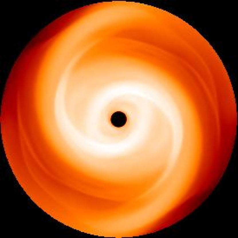
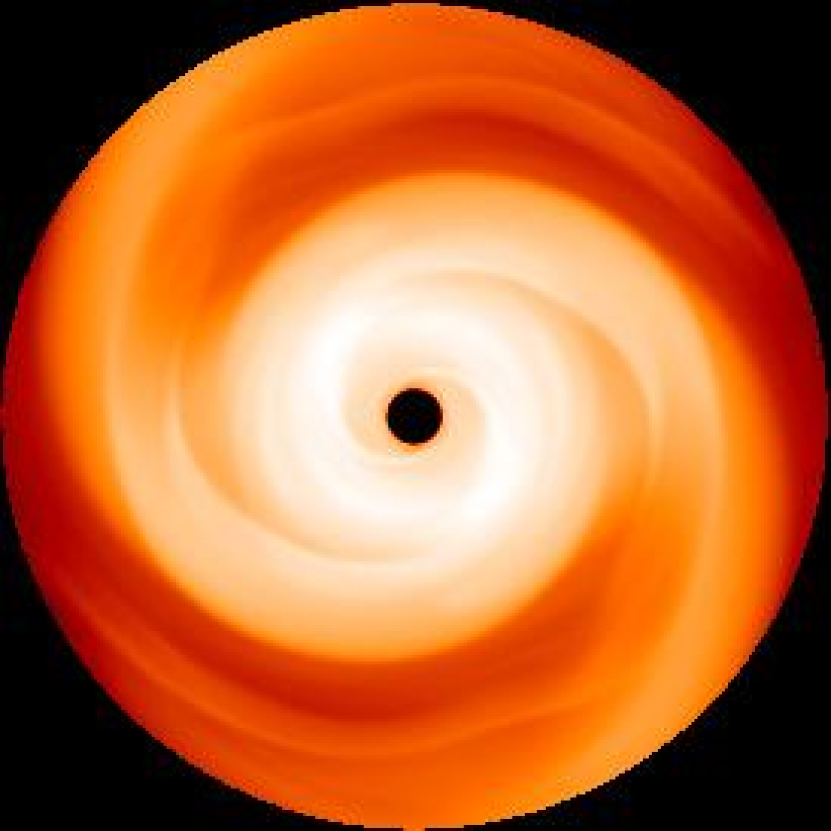
Figure 9: Logarithm of the density in the equatorial plane for run T2 at $t=4.95$ (left panel) and $t=5.09$ (right panel). These snapshots correspond to a maximum and a minimum of the gravitational stress, respectively. The spiral arms are sharp and clear at $t=4.95$, whereas they appear blurred at $t=5.09$.

Figure 10: Time evolution of the mass accretion rate (mass per unit of time) onto the central mass for run T2. As expected, the accretion rate oscillates with the same period as the gravitational stress.

In figure 11, we compare the evolution of the Maxwell stress in models T2 and T2^∗ (for which only the first $6$ orbits, during which $m_{max}=0$, are plotted). In contrast to the gravitational stress, the Maxwell stress is significantly larger when the disk is gravitationally unstable. This appears to be due to the systematic compression of the magnetic field lines along the spiral arms, as opposed, say, to an increase of the level of turbulent fluctuations. When the gravitational instability disappears after about $7$ orbits in model T2, for example, the Maxwell stress decreases to the same value as in model T2^∗.

As in the hydro model HD, the Toomre $Q$ parameter rises throughout the body of the disk over the course of the simulation (as mass is transported toward the inner region), until the gravitational instability ceases. But even by $t\simeq 8$, when there is no longer any gravitational transport, $Q$ is still larger in model HD than in model T2. This is because the gravitational instability is stronger in the hydrodynamical case, and the disk is depleted more rapidly.

Figure 11: Time evolution of the volume averaged Maxwell stress tensor for runs T2^∗ (dashed line), before gravitational transport is turned on, and T2 (dotted line). The Maxwell stress is larger when the disk is gravitationally unstable. This appears to be due to a compression of the magnetic field lines along the spiral arms. When the disk in model T2 becomes gravitationally stable (after $t\simeq 7$), the Maxwell stress decreases down to the same value as in model T2^∗.

To check the sensitivity of these results to our choice of initial conditions, we conducted the following experiment. In model T2^∗, the input parameters are the same as in model T2, but the non–axisymmetric part of $\Phi_{s}$ is included only after 6 orbits, i.e. only after MHD turbulence has been firmly established. Figure 12 shows the time evolution of the volume averaged Maxwell and gravitational stress tensors for run T2^∗. Until $t=7$, the development of MHD turbulence is the same as in model T1. However, in the time interval $t=7$–8, i.e. after gravitational instabilities have developed, $\langle T_{r\phi}^{Max}\rangle$ decreases to reach about one third of its value at $t=7$. The reason of this decline is not completely clear. One possibility may be that the compression of the (randomized) magnetic field in the spiral arms leads to more efficient reconnection of the field lines. Another possibility is that gravitational stresses feed off the density fluctuations generated by the MRI, thereby indirectly coupling the magnetic and gravitational energies. In any case, this behavior stands in contrast with was observed in run T2, where gravitational instabilities developed while the magnetic field was still ordered. In model T2^∗, the gravitational stress tensor is roughly a factor of $2$ smaller than in model T2, but shows the same periodic variations.

Figure 12: Time evolution of the volume averaged Maxwell (solid line) and gravitational (dashed line) stress tensors for run T2^∗. In this run, the non–axisymmetric part of $\Phi_{s}$ is included only after 6 orbits, i.e. only after MHD turbulence has been firmly established. The development of gravitational instabilities coincides with a significant decrease of the Maxwell stress tensor. This may be due to reconnection of the (randomly oriented) field lines in the spiral arms. The gravitational stress tensor has the same amplitude and periodic variations as in run T2.

Our next comparison run, model T3, differs from model T2 only in the number $m_{max}$ of fourier coefficients in the expansion of $\Phi_{s}$. (T3 has $m_{max}=16$, T2 has $m_{max}=8$.) Once again, very similar results emerge, and the choice of $m_{max}$ does not appear to be critical (cf. § 4.3.3).

To summarize: the evolution of a purely toroidal field in a gravitationally unstable disk leads to a reduction and strong periodicity in the gravitational stress (compared with a purely hydrodynamical model). Compared with gravitationally stable models, the Maxwell stress is larger or smaller depending repsectively on whether gravitational instabilities develop at the same time as MHD turbulence (magnetic field alignment in spiral arms) or after turbulence is established (reduction in magnetic stress as gravitational stress develops). The behavior of an initial poloidal field is considered next.

4.3.2 Initial Poloidal Field: Model P2

Do our toroidal field findings extend to poloidal field behavior? To answer this question, we begin with an initial poloidal field, calculated as in section 4.2.2 above. Again, we start with $\langle\beta\rangle=300$. Except for the initial field geometry, model P2 is the same as model T2.

Figure 13 shows the evolution of the gravitational stress tensor for both models P2 and HD (this is the equivalent of figure 8). As in the case of a toroidal field, a non–axisymmetric $m=2$ spiral grows and becomes nonlinear in model P2. The fact that gravitational instabilities develop earlier in model P2 than in models T2 and HD (see figures 8 and 13) appears to be due to the fact that the strong linear magnetic instability associated with the poloidal field produces large perturbations of the density. Once again, we find that the gravitational stress is smaller than in model HD, and varies periodically with time with a period $\sim 0.38$ somewhat larger than for model P2.

Figure 13: Time evolution of the volume averaged gravitational stress tensor for models HD (solid line) and P2 (dotted line). The gravitational stress in model P2 is smaller than in model HD and varies periodically with time.

Figure 14 shows the evolution of the Maxwell stress for models P1 and P2 (this is the equivalent of figure 11). Once again, the Maxwell stress is larger when the disk is gravitationally unstable and gravitational instabilities develop at the beginning of the run (model P2).

Since the state of MHD turbulence in a saturated disk is the same whether an initial poloidal or toroidal field is used, we have not run a case “P2^∗” with the non–axisymmetric part of $\Phi_{s}$ added later. Such a run is expected to be very similar to T2^∗, since the initial turbulent states are similar.

The history of run P2 and the above argument together suggest that toroidal and poloidal initial fields behave very similarly.

Figure 14: Time evolution of the volume averaged Maxwell stress tensor for models P1 (dashed line) and P2 (dotted line). The Maxwell stress is larger when the disk is gravitationally unstable and gravitational instabilities develop at the beginning of the run.

4.3.3 Modal analysis

The full MHD simulations described above suggest that a general feature of the evolution of gravitationally unstable turbulent disks is a periodic modulation of the gravitational stress. To understand the reason for this modulation, we now analyse in more detail the unstable modes that appear in models HD, T2 and P2. We are in particular interested in determining the power spectrum as a function of mode frequency $\sigma$. Following Papaloizou & Savonije (1991), we Fourier transform in time at each radial zone $r$ and at a fixed azimuth $\phi_{0}$ the function $\rho(r,\phi_{0},t)$. To get the spectral time evolution, we carry out each Fourier transform over a series of 4 distinct time intervals. The number of time-steps used in each time interval gives a finite frequency resolution $d\sigma/2\pi=0.3$. The contours of constant power are then plotted as a function of frequency and radius for the various time intervals.

Figure 15 shows the contours for model HD. The different panels correspond to different time intervals. In the first panel, i.e. at time $t\simeq 2.4$, we see the presence of a mode with frequency $\sigma/2\pi=2.5$ which extends over the whole disk. Its amplitude is small, peaking at about $3\times 10^{-2}$. This mode is still present in the second panel, at time $t\simeq 3.4$, with a similar amplitude structure. However, a second low frequency mode with $\sigma/2\pi=1$ (i.e. with a corotation radius at the disk initial outer edge) is now apparent. Its amplitude is significant only in the disk outer parts, where it peaks at 0.2. This mode subsequently grows and completely dominates the high frequency ($\sigma/2\pi=2.5$) mode in the third panel, i.e. at $t\simeq 4.4$. There its amplitude peaks at 0.7. This mode can of course be identified with the two–arm spiral seen in figure 4. At $t=4.4$ the mode is non–linear. Its amplitude does not increase further, as can be seen in the fourth and last panel, i.e. at $t\simeq 5.4$. At this later time, only the frequency of the mode has changed. It is now around 1.5. Both the finite frequency resolution $d\sigma$ and the increase of the central mass due to accretion may account for this shift in frequency. A third mode with a frequency twice that of the low frequency mode is seen in the last two panels. The relationship between the frequencies of these two modes and the fact that their radial structure is very similar suggests that they are harmonics of each other.

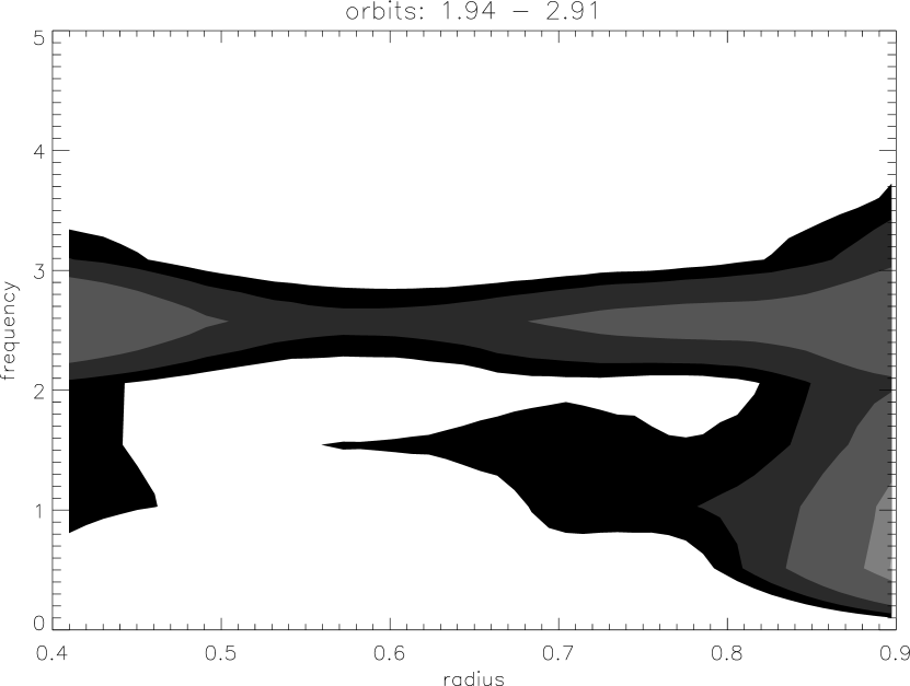
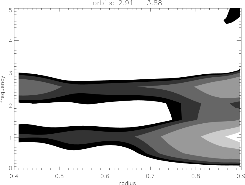
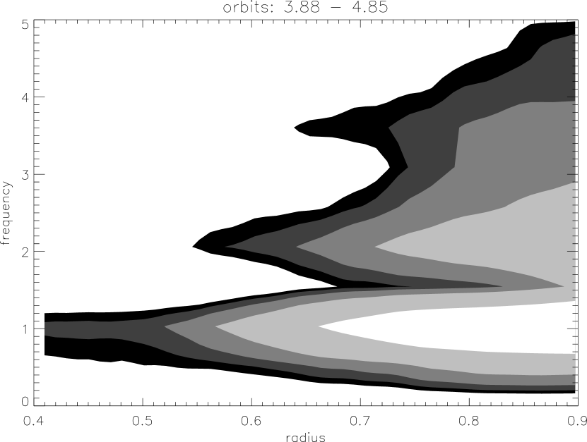
Figure 15: Contours of constant Fourier power as a function of dimensionless mode frequency $\sigma/2\pi$ (vertical axis) and radius $r$ (horizontal axis) for model HD. The different panels correspond to the time intervals 1.94–2.91 (upper left), 2.91–3.88 (upper right), 3.88–4.85 (lower left) and 4.85–5.83 (lower right). The contour levels in each of these panels are, in unit $10^{-2}$: (0.22; 0.29; 0.44; 0.87; 1.1; 1.6; 3.2), (2.1; 2.6; 3.4; 5.2; 10; 15), (8.4; 11; 14; 21; 42) and (9.4; 12; 16; 23; 47; 62), respectively. One mode (a two–arm spiral) dominates the spectrum in the non–linear stage (third panel), with a frequency $\sigma/2\pi=1$.

Figure 16 shows the contour plots for model T2. In the first panel, at $t\simeq 2.4$, there is no dominant mode. Instead, there is a large number of high frequency (with mostly $\sigma/2\pi=1.3$–3.8) perturbations. The amplitude of these fluctuations is a few times $10^{-2}$. They are associated with the growing MRI. In the second panel, at $t\simeq 3.4$, two modes emerge, but their amplitude is still rather low. However, these modes subsequently grow and are clearly seen with a larger amplitude in the third panel, at $t\simeq 4.4$. One of these modes has a frequency $\sigma/2\pi=1$ and is the same as that seen in the hydrodynamical simulations. Its corotation radius is located at the disk initial outer edge. Its amplitude peaks at a value of about 0.5 in the outer parts of the disk. The other mode has a frequency $\sigma/2\pi=2.5$ and an amplitude $\sim 0.2$ constant over the whole disk. In particular, its amplitude in the disk inner parts is larger than that of the other mode. This mode is probably the same as that seen with a lower amplitude at early times in the hydrodynamical simulations (panels 1 and 2 of figure 15). This suggests that this mode is a disk eigenmode which is excited in model T2 by the high frequency motions associated with the turbulence. We expect nonlinear coupling between these two modes to give rise to beat oscillations, i.e. oscillations with a frequency being a linear combination of the frequencies of the two modes. We have noted above that the gravitational stress tensor in model T2 oscillates with a period $\sim 0.28$. This is consistent with the frequency of the oscillations being $\sigma/2\pi\simeq m(\sigma_{\rm HF}-\sigma_{\rm BF})=3$, where $\sigma_{\rm HF}$ and $\sigma_{\rm BF}$ are the frequencies of the high and low–frequency modes, respectively. This suggests that the oscillations of the gravitational stress tensor result from a nonlinear coupling between these two modes.

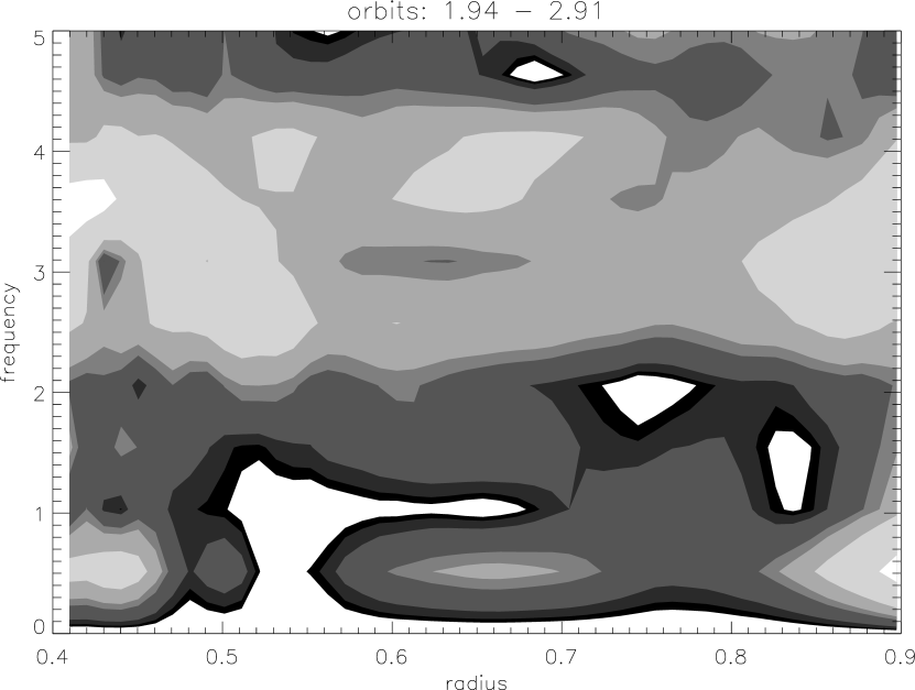
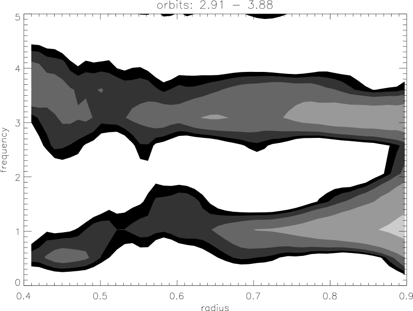
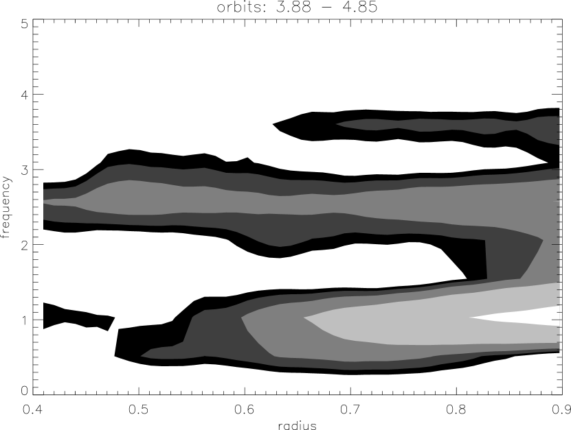
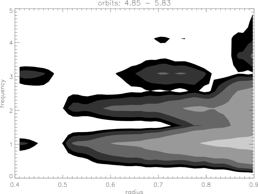
Figure 16: Same as figure 15 but for model T2. The contour levels in each panel are the same as in figure 15. Here two modes dominate the spectrum in the nonlinear phase (third panel), with frequencies $\sigma/2\pi=1$ and $\sigma/2\pi=2.5$, respectively.

Figure 17 shows the contour plots for model P2 in the time interval 2.72–3.88. the situation is similar to model T2. Here again two modes of comparable amplitude are present. One of this mode has a frequency $\sigma/2\pi=1$ and can be identified with the mode which emerges in the hydrodynamical simulations. The other mode has a frequency $\sigma/2\pi=2.1$. Given the finite frequency resolution $d\sigma/2\pi$, this second mode may be the same as that identified in model T2. However, it may also be a different mode with a lower frequency. In any case, the situation is qualitatively the same here as in model T2. Since the two modes have comparable amplitude, they interact nonlinearly, which results in a periodic modulation of the gravitational stress.

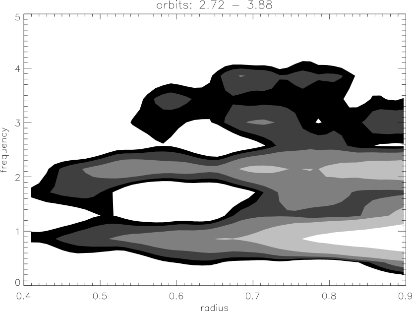
Figure 17: Same as figure 15 but for model P2 and only in the time interval 2.72–3.88. The contour levels used here are, in unit $10^{-2}$: (5.1; 6.4; 8.5; 13; 25).

We now vary some of the parameters of model T2 in order to examine the sensitivity of these physical results to the numerical input parameters. Figure 18 shows the contour plots for model T2_low in the time interval 2.72–3.88. The resolution for this run in the radial and vertical directions is half that of model T2. The similarity between this plot and the third panel of figure 16 demonstrates that our results do not depend strongly on the numerical resolution. Figure 19 is the same as figure 18 but for model T3. Again, it is very similar to the third panel of figure 16. Since, in model T3, only the parameter $m_{max}$ is different from model T2, figure 19 suggests that the limited number of Fourier components included in the calculation of the self–gravitating potential does not qualitatively affect the main physical results presented in this paper.

In conclusion, models P2, T2_low and T3, taken together, suggest that the physical results described in this paper are insensitive to both the numerical setup of the simulations and the initial magnetic field topology.

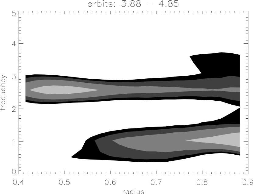
Figure 18: Same as figure 15 but for model T2_low and only in the time interval 2.72–3.88. The contour levels used here are, in unit $10^{-2}$: (5.1; 6.4; 8.5; 13; 25).

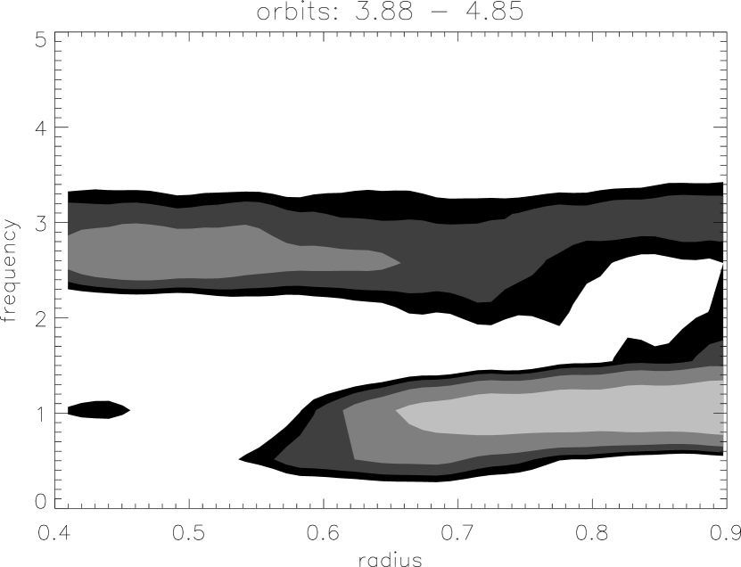
Figure 19: Same as figure 15 but for model T3 and only in the time interval 2.72–3.88. The contour levels used here are, in unit $10^{-2}$: (5.1; 6.4; 8.5; 13; 25).

5 Discussion

In this paper, we have presented the first 3D numerical simulations of the evolution of self–gravitating and magnetized disks. We have investigated disks in which only gravitational or magnetic instabilities develop, and disks in which both types of instabilities occur.

When no magnetic field is present, self-gravitating disks are unstable when the Toomre $Q$ parameter is close to unity. The spectrum of unstable modes in that case is dominated by a large scale two–arm spiral whose corotation radius is located near the disk outer edge. The instability is due to the interaction between waves which propagate near the disk outer boundary and inside the inner Lindblad resonance (ILR), respectively (Papaloizou & Savonije, 1991).

When a magnetic field is present, two large scale modes grow in the disk. They both have $m=2$. One of this mode is the same as that seen in the hydrodynamical simulations. The second mode has a higher frequency. The ILR of the low–frequency mode, which is at $r\simeq 0.6$, is very close to the corotation radius of the high–frequency mode, which is at $r\simeq 0.5$. Such a pair of modes was seen in the hydrodynamical calculations of self–gravitating disks performed by Papaloizou & Savonije (1991). There, both modes were unstable because of the particular vortensity profile. In our simulations, in the absence of magnetic field, only the low–frequency mode is unstable. The high–frequency mode seems to be part of the spectrum of normal modes in that case, but it does not grow. The presence of MHD turbulence does not modify the spectrum of large scale (comparable to the disk radius) modes, as it acts on scales limited by the disk thickness. However, the fact that the high–frequency mode is unstable in the MHD simulations suggests that turbulence acts as a source for high–frequency oscillations.

Nonlinear coupling between these two modes leads to an oscillation of the gravitational stress tensor. Note that such a coupling between two modes with coinciding resonances has been suggested to explain some of the features seen in numerical simulations of galactic disks by Tagger et al. (1987). These authors argued that the proximity of the resonances made the coupling very efficient. The oscillation of the gravitational stress tensor is accompagnied by the periodic disappearance of the spiral arms in the disk. Also, the peak value of this stress is decreased by about half compared to the hydrodynamical simulations.

The results reported here are robust and do not depend on the geometry of the magnetic field. They have important consequences for disks around AGN and protoplanetary disks. They first show that accretion of a self–gravitating disk onto the central star is slowed down when a magnetic field is present. They also show that the accretion is time–dependent, with a characteristic timescale for the variability being on the order of a fraction of the dynamical timescale at the outer edge of the region where the instabilities develop.

As mentioned in the introduction, protoplanetary disks are probably self–gravitating in the early phases of their evolution. For a disk of about 100 AU, the work presented here suggests variability on a timescale $\sim 10^{3}$ years. The periodicity in the spatial distribution of knots in jets emanating from such objects is in the range 10–$10^{3}$ years (Reipurth, 2000), and is usually thought of as being produced by a time–dependent accretion in the central parts of the disk. The simulations presented in this paper suggest that periodic modulations of the accretion rate might well be the result of the interplay between gravitational instabilities and MHD turbulence, a far from obvious source. Note that the first detection of near–IR variability in a sample of Class I protostars was performed recently by Park & Kenyon (2002). However, the poor time coverage of their data prevents a useful measure of the variability timescales to be extracted.

Disks around AGN display time–dependent phenomena on a large range of timescales (Ulrich et al., 1997). The dynamical timescale for a disk orbiting a $10^{8}$ solar masses black hole at $10^{-2}$ parsecs is 9.3 years, and variations are observed on timescales up to years. This again is consistent with the processes described in this paper.

References

- Abramowitz & Stegun (1965) Abramowitz, M., & Stegun, I. 1965, Handbook of Mathematical Functions with Formulas, Graphs, and Mathematical Tables (New York: Dover)
- Balbus & Hawley (1991) Balbus, S., & Hawley, J. 1991, ApJ, 376, 214
- Balbus & Hawley (1998) —. 1998, Rev.Mod.Phys., 70, 1
- Balbus & Papaloizou (1999) Balbus, S., & Papaloizou, J. 1999, ApJ, 521, 650
- Balbus (2003) Balbus, S. A. 2003, ARA&A, 41, 555
- Binney & Tremaine (1987) Binney, J., & Tremaine, S. 1987, Galactic dynamics (Princeton University Press)
- Boss (1998) Boss, A. P. 1998, ApJ, 503, 923
- Boss (2002) Boss, A. P. 2002, ApJ, 576, 462
- Cohl & Tohline (1999) Cohl, H. S., & Tohline, J. E. 1999, ApJ, 527, 86
- Fromang et al. (2004) Fromang, S., Balbus, S. A., & De Villiers, J. P. 2004, ApJ, submitted (Paper I)
- Fromang et al. (2002) Fromang, S., Terquem, C., & Balbus, S. A. 2002, MNRAS, 329, 18
- Gammie (1996) Gammie, C. F. 1996, ApJ, 457, 355
- Goodman (2003) Goodman, J. 2003, MNRAS, 339, 937
- Goodman & Xu (1994) Goodman, J., & Xu, G. 1994, ApJ, 432, 213
- Hachisu (1986) Hachisu, I. 1986, ApJS, 62, 461
- Hawley & Stone (1995) Hawley, J., & Stone, J. 1995, Comput. Phys. Commun., 89, 127
- Hawley (2000) Hawley, J. F. 2000, ApJ, 528, 462
- Hawley (2001) —. 2001, ApJ, 554, 534
- Hawley & Balbus (1991) Hawley, J. F., & Balbus, S. A. 1991, ApJ, 376, 223
- Hirsch (1988) Hirsch, C. 1988, Numerical Computation of Internal and External Flows - Volume 1, Fundamentals of Numerical Discretization. (Wiley)
- Laughlin & Bodenheimer (1994) Laughlin, G., & Bodenheimer, P. 1994, ApJ, 436, 335
- Laughlin et al. (1997) Laughlin, G., Korchagin, V., & Adams, F. 1997, ApJ, 477, 410
- Mayer et al. (2002) Mayer, L., Quinn, T., Wadsley, J., & Stadel, J. 2002, Science, 298, 1756
- Menou & Quataert (2001) Menou, K., & Quataert, E. 2001, ApJ, 552, 204
- Papaloizou & Nelson (2003) Papaloizou, J., & Nelson, R. 2003, MNRAS, 339, 983
- Papaloizou & Savonije (1991) Papaloizou, J., & Savonije, G. 1991, MNRAS, 248, 353
- Pickett et al. (1998) Pickett, B., Casse, P., Durisen, R., & Link, R. 1998, ApJ, 504, 468
- Pickett et al. (2000) Pickett, B., Cassen, P., Durisen, R., & Link, R. 2000, ApJ, 529, 1034
- Pickett et al. (1996) Pickett, B., Durisen, R., & Davis, G. 1996, ApJ, 458, 714
- Pickett et al. (2003) Pickett, B., Mejia, A., Durisen, R., Cassen, P., Berry, D., & Link, R. 2003, ApJ, 590, 1060
- Reipurth (2000) Reipurth, B. 2000, AJ, 120, 3177
- Rice et al. (2003) Rice, W., Armitage, P., Bonnell, I., Bate, M., Jeffers, S., & Vine, S. G. 2003, MNRAS, 339, 1025
- Sano et al. (2000) Sano, T., Miyama, S. M., Umebayashi, T., & Nakano, T. 2000, ApJ, 543, 486
- Shakura & Sunyaev (1973) Shakura, N. I., & Sunyaev, R. A. 1973, A&A, 24, 337
- Steinacker & Papaloizou (2002) Steinacker, A., & Papaloizou, J. 2002, ApJ, 571, 413
- Tagger et al. (1987) Tagger, M., Sygnet, J. F., Athanassoula, E., & Pellat, R. 1987, ApJ, 318, L43
- Tohline & Hachisu (1990) Tohline, J., & Hachisu, I. 1990, ApJ, 361, 394
- Toomre (1964) Toomre, A. 1964, ApJ, 139, 1217
- Ulrich et al. (1997) Ulrich, M., Maraschi, L., & Urry, C. M. 1997, ARA&A, 35, 445
- Woodward et al. (1994) Woodward, J. W., Tohline, J. E., & Hachisu, I. 1994, ApJ, 420, 247