Long-time evolution of magnetic fields in relativistic GRB shocks

Abstract

We investigate the long-time evolution of magnetic fields generated by the two-stream instability at ultra- and sub-relativistic astrophysical collisionless shocks. Based on 3D PIC simulation results, we introduce a 2D toy model of interacting current filaments. Within the framework of this model, we demonstrate that the field correlation scale in the region far downstream the shock grows nearly as the light crossing time, $\lambda(t)\sim ct$, thus making the diffusive field dissipation inefficient. The obtained theoretical scaling is tested using numerical PIC simulations. This result extends our understanding of the structure of collisionless shocks in gamma-ray bursts and other astrophysical objects.

1. Introduction

Internal and external shocks in gamma-ray bursters (GRBs), internal shocks produced in jets of micro- and normal quasars and in active galactic nuclei jets, shocks in supernovae remnants, merger shocks in galaxy clusters and large scale structure, — all of them represent a single class of strong collisionless shocks. The theoretical prediction that the counterstreaming instability operating at the shock produces strong magnetic fields (Medvedev & Loeb 1999) has recently been confirmed in a number of state-of-the-art numerical sumulations (Silva, et al. 2003; Frederiksen, et al. 2004; Nishikawa, et al. 2003; Saito & Sakai 2004; Kazimura, et al. 1998). In this paper we investigate the long-time, nonlinear evolution of the produced fields. The knowledge of the field dynamics downstream the shock is crucial for our understanding of the shock particle acceleration, as well as the spectral properties (e.g., variability) of radiation produced at astrophysical shocks.

2. The model

Fully 3D PIC numerical simulations of the shocks demonstrate that the generated magnetic fields are associated with a quasi-two-dimensional distribution of current filaments (Silva, et al. 2003). Hence we suggest the following toy model.

We consider straight one-dimensional current filaments oriented in the vertical, $\hat{z}$, direction. Initially, all filaments are identical: the initial diameter of them is $D_{0}$, their initial mass per unit length is $\mu_{0}\simeq mn(\pi D_{0}^{2}/4)$, where $m$ is the mass of plasma particles (e.g., electrons) and $n$ is their number density. Each filament carries current $I_{0}$ in either positive or negative $\hat{z}$-direction. The net current in the system is set to zero, i.e., there are equal numbers of positive and negative current filaments. We also assume that the initial separation (the distance between the centers, see Fig. 2) of the filaments $d_{0}$ is comparable to their size, $d_{0}\simeq 2D_{0}$. Finally, no external homogeneous magnetic field is present in the system.

2.1. Single filament dynamics

Initially, the filaments are at rest and their positions in space are random. This configuration is unstable because opposite currents repel each other, whereas like currents are attracted to each other and tend to coalesce and form larger current filaments. The characteristic scale of the magnetic field will accordingly increase with time. We study this process quantitatively using the toy model of two interacting filaments. There are two limiting cases: (i) when the characteristic velocity of the filaments during the coalescence process is much smaller than the speed of light and (ii) when these velocities are comparable. We consider these cases separately.

2.1.1 Nonrelativistic motion

The magnetic field produced by a straight filament is $B_{0}(r)=2I_{0}/(cr)$, where $r$ is the cylindrical radius. The force per unit length acting on the second filament is $dF/dl=-B_{0}I_{0}/c$. Since $dF/dl=\mu\ddot{x}$, where $x$ is the position in the center of mass frame and “overdot” denotes time derivative, we write the equation of motion as follows:

$$\ddot{x}=-\frac{2I_{0}^{2}}{c^{2}\mu_{0}}\,\frac{1}{x},$$ (1)

where we used that $r=2x$ and the reduced mass $\mu_{r}=\mu_{0}/2$. We define the coalescence time as the time required for the filaments, which are initially at rest, to cross the distance between them and “touch” each other, which happens when the distance between their centers becomes equal to $D_{0}$, i.e., when $x=D_{0}/2$. The coalescence time, as it is defined above, is independent of the details of the merging process itself, which involves rather complicated dynamics associated with the redistribution of currents. Quite obviously, the interaction between the filaments is the weakest at large distances $x\sim x_{0}\sim d_{0}/2$. Hence, the coalescence rate is limited by the filament motions at the largest scales. The coalescence time can be readily estimated from Eq. (1), assuming that $x\sim x_{0}\sim d_{0}/2$ and $\ddot{x}\sim(d_{0}/2)\tau_{0}^{-2}$, as follows:

$$\tau_{0,NR}\sim\left({D_{0}^{2}c^{2}\mu_{0}}/({2I_{0}^{2}})\right)^{1/2}.$$ (2)

The above estimate is valid as long as the motion is nonrelativistic. The maximum velocity of a filament is at the time of coalescence, $x=D_{0}/2$:

$$v_{m0}\sim D_{0}/2\tau_{0}\sim I_{0}/(c\sqrt{2\mu_{0}}).$$ (3)

It must always be much smaller than the speed of light.

It turns out that Eq. (1) can be solved exactly in terms of time as a function of the filament separation:

$$t(x)={\sqrt{\pi\mu_{0}}\,cx_{0}}/({2I_{0}})\,\textrm{erfc}\!\left(\sqrt{-\ln(x/x_{0})}\right),$$ (4)

where $x_{0}=x(0)$ and $\textrm{erfc}(y)=2\pi^{-1/2}\int_{y}^{\infty}e^{-\eta^{2}}d\eta$ is the complimentary error function. The coalescence time can be calculated exactly:

$$\tau_{0,NR}={\sqrt{\pi\mu_{0}}\,cD_{0}}/({4I_{0}})\,\textrm{erfc}\!\left(\sqrt{\ln 2}\right)\approx 0.11\sqrt{\mu_{0}}cD_{0}/I_{0},$$ (5)

which is shorter than our estimate, Eq. (2), by a factor of seven. The velocity as a function of position is

$$v(x)={2I_{0}}/({c\sqrt{\mu_{0}}})\,\sqrt{-\ln(x/x_{0})}.$$ (6)

Consequently, the maximum velocity is

$$v_{m0}={2I_{0}}/({c\sqrt{\mu_{0}}})\,\sqrt{\ln 2}\approx 1.67I_{0}/(c\sqrt{\mu_{0}}).$$ (7)

2.1.2 Relativistic motion

If the motion of a filament during the merger becomes relativistic, the separation cannot decrease faster than as $t(x)\simeq x/c$. Therefore, the coalescence time will be

$$\tau_{0,R}\simeq(d_{0}/2)/c=D_{0}/c.$$ (8)

2.2. Collective dynamics of filaments

We now consider the filament coalescence as a hierarchical process. Suppose that initially the system contains $N_{0}$ current filaments, with an average separation $d_{0}\sim 2D_{0}$. Each of the filaments carries current $I_{0}$, its diameter is $D_{0}$ and its mass per unit length is $\mu_{0}$. For simplicity, we asssume that filaments coalesce pairwise.

Having the original “zeroth generation” of filaments merged (the process takes about $\tau_{0,NR}$ or $\tau_{0,R}$ to complete), the system will now contain $N_{0}/2$ of “first generation” filaments. Each of these filaments carries current $I_{1}=2I_{0}$, has mass per unit length $\mu_{1}=2\mu_{0}$, and the separation between them is $d_{1}=\sqrt{2}d_{0}$ (because the two dimensional number density of filaments decreased by 2). Since $\mu\propto D^{2}$, the filament size also increases as $D_{1}=\sqrt{2}D_{0}$. Remarkably, this new configuration is identical to the initial one, but with the re-scaled parameters. Hence, the coalescence process is self-similar. The produced first generation filaments will be interacting with each other and merge again to yield the second generation. The coalescence process will then continue in a self-similar way. Note that the coalescence times at each stage are not necessarily the same.

At the $k$-th merger level, i.e., after $k$ pairwise mergers, the filament current, its mass per unit length and its size are

$$I_{k}=2^{k}I_{0},\qquad\mu_{k}=2^{k}\mu_{0},\qquad D_{k}=2^{k/2}D_{0},$$ (9)

whereas the filament separation is $d_{k}\sim D_{k}/2$. The coalescence time at $k$-th level may be estimated in the way described in the prevous section. Using Eq. (2) or (5) and Eq. (8), we obtain

$$\tau_{k,NR}=\tau_{0,NR},\qquad\tau_{k,R}=2^{k/2}\tau_{0,R}.$$ (10)

Since the coalescence time is independent of $k$ while the filaments are non-relativistic, whereas the distance between them increases, the typical velocities of the merging filaments grow with time and, will approach $c$. From Eq. (7), we obtain $v_{m,k}=2^{k/2}v_{m0}$. The transition from the non-relativistic regime to the relativistic one occurs after about $k_{*}$ mergers:

$$k_{*}=2\log_{2}(c/v_{m0}),$$ (11)

where $v_{m0}$ is set by the initial state of the system, Eq. (7).

Our primary interest is the evolution of the transverse correlation length of the magnetic field. With the filamets being randomly distributed in space, the characteristic scale on which the magnetic field fluctuates is about half the distance between the filaments, i.e., $\lambda_{B,k}\simeq d_{k}/2$. Thus,

$$\lambda_{B,k}\simeq 2^{k/2}D_{0}.$$ (12)

Finally, it is instructive to present the evolution of the parameters as a function of physical time, $t$, rather than the merger level, $k$. Apparently, it takes $t=\sum_{k^{\prime}=0}^{k}\tau_{k^{\prime}}$ to complete $k$ mergers, where $\tau_{k}$ is given by Eq. (10). This equation implicitly defines $k(t)$. In the non-relativistic case, the solution to this equation is obvious: $k=t/\tau_{0}$, because $\tau_{0}$ is independent of $k$. In the relativistic case, the sum of the series is easily calculated using that $\sum_{i=0}^{n}a^{i}=(a^{n+1}-1)/(a-1)$. Thus, for the non-relativistic and relativistic cases respectively, the solution to the equation $t=\sum_{k^{\prime}=0}^{k}\tau_{k^{\prime}}$ reads

$$k = {t}/{\tau_{0,NR}},$$ (13)

$$k = 2\log_{2}\left[({t}/{\tau_{0,R}})(\sqrt{2}-1)+1\right]-1.$$ (14)

Thus, the magnetic field correlation length increases as a function of time as

$$\lambda_{B}(t)=D_{0}2^{{t}/({2\tau_{0,NR}})},\qquad\lambda_{B}(t)\simeq ct,$$ (15)

in the non-relativistic and relativistic regimes, respectively. Note that the last expression is an approximation at large times $t\gg\tau_{0,R}$, i.e., at large $k\gg 1$.

3. Application to collisionless shocks

The growth rate and the saturation level of the field generated at shocks depend on the composition of the outflowing ionized gas (Medvedev & Loeb 1999; Silva, et al. 2003; Frederiksen, et al. 2004). The gas composition in the cosmological outflows is not generally known. Considering the interaction of the ejecta with the interstellar medium, — the external shock, — it is quite reasonable to assume that the shock is propagating through an electron-proton plasma. In contrast, the ejecta itself, where internal shocks occur, may be either dominated by electron-positron pairs (leptonic jet) or by electrons and protons (baryonic jet) with or without $e^{-}e^{+}$-pair sub-population.

Here, we will consider a general case of the ejecta containing several species, labeled by the subscript $s$. We assume that the species have different masses $m_{s}$, but their charges, by the absolute value, are equal to $e$. In general, each species has the bulk Lorentz factor (in the center of mass frame) $\gamma_{s}$ and the thermal Lorentz factor $\bar{\gamma}_{s}$, the latter represents the random velocites of the particles (initially, $\bar{\gamma}_{s}<\gamma_{s}$). When the instability shuts off, the particles are randomized over the pitch angle, hence $\bar{\gamma}_{s}\simeq\gamma_{s}$. In the context of astrophysical outflows, we assume that all the species have the same $\gamma_{s}=\Gamma$ and $\bar{\gamma}_{s}\sim\Gamma$, where $\Gamma$ is either the Lorentz factor of the external shock in observer’s frame, or the relative Lorentz factor of the two colliding shells measured in the frame comoving with the ejecta. In the latter case, the ejecta itself moves relativistically in observer’s frame with the Lorentz factor $\Gamma_{\rm ej}$.

It is convenient to introduce the equipartition parameter for each species:

$$\epsilon_{B,s}=B^{2}_{s}/(8\pi n_{s}\gamma_{s}m_{s}c^{2}),$$ (16)

where $B_{s}$ is the strength of the magnetic field produced by the instability operating on the species $s$, $n_{s}$ is the number density of particles (both parameters are measured in the shock comoving frame). The equipartition parameter describes the efficiency of the magnetic field generation process, i.e., what fraction of the total kinetic energy of the particles of each species goes into the magnetic field energy. Note that this definition of the equipartition parameter is different from the commonly used definition, which describes the fraction of the total kinetic energy of the ejecta (summed over all species) that goes into magnetic field. We define the plasma and Larmor frequencies as

$$\omega_{p,s} = \left(4\pi e^{2}n_{s}/\gamma_{s}m_{s}\right)^{1/2},~{}$$ (17)

$$\omega_{B,s} = eB_{s}/\gamma_{s}m_{s}c.$$ (18)

For convenience, we also introduce their “nonrelativistic” counterparts $\hat{\omega}_{p,s}\equiv\omega_{p,s}\gamma_{s}^{1/2}$ and $\hat{\omega}_{B,s}\equiv\omega_{B,s}\gamma_{s}$. It is useful to remember the following relation:

$${\omega_{B,s}}/{\omega_{p,s}}=\sqrt{2\epsilon_{B,s}}.$$ (19)

We may now represent the main results of Section 2 in terms of plasma parameters. First, the initial separation between the filaments, $D_{0}$, must be comparable to the characteristic correlation length of the magnetic field produced by the instability. This length at the onset of the instability is, in turn, set by the wavenumber of the fastest growing mode (Medvedev & Loeb 1999): $\lambda_{s}\simeq\bar{\gamma}_{s}^{1/2}c/\hat{\omega}_{p,s}$, which is a factor of $(\bar{\gamma}_{s}/\gamma_{s})<1$ smaller than the relativistic skin depth, $c/\omega_{p,s}$. However, we cannot set this scale $\lambda_{s}$ as $D_{0}$ because, as indicated by 3D PIC $e^{-}e^{+}$ simulations (Silva, et al. 2003), $\epsilon_{B}$ is not constant in time at the beginning of the nonlinear filament interaction (at $t\sim 10\omega_{p,s}^{-1}$). Hence the analysis of Section 2 is not applicable in such a regime. In fact, it takes few plasma times, $\omega_{p,s}^{-1}$, in their simulations for $\epsilon_{B}$ to attain its asymptotic value. The field correlation scale at this moment ($t\sim 15\omega_{p,s}^{-1}$) is somewhat larger than $\lambda_{s}$. We include this uncertainty via the parameter $\eta>1$ as follows:

$$D_{0}=\eta\,({c}/{\omega_{p,s}})=\eta\,({c\sqrt{\Gamma}}/{\hat{\omega}_{p,s}}).$$ (20)

Second, using $\oint{\bf B}\cdot d{\bf l}=(4\pi/c)I$, we express the current $I_{0}$ in terms of the equipartition parameter, $\epsilon_{B,s}$, as

$$I_{0}=\eta\Gamma\sqrt{{\epsilon_{B,s}}/{2}}\,({m_{s}c^{3}}/{e}).$$ (21)

Third, the mass per unit length of a filament must take into account that the particle thermal motion is relativistic, hence the masses are $\bar{\gamma}_{s}m_{s}\sim\Gamma m_{s}$. We obtain

$$\mu_{0}=\Gamma m_{s}n_{s}\left(\pi D_{0}^{2}/4\right).$$ (22)

The temporal evolution of the field correlation scale is determined by Eq. (15), where $\tau_{0,NR}$ is given by (5). The coalescence time may be written as

$$\tau_{0,NR}=\frac{\alpha_{\tau}\eta}{2}\,\omega_{B,s}^{-1}=\frac{\alpha_{\tau}\eta}{\sqrt{8\epsilon_{B,s}}}\,\omega_{p,s}^{-1}\sim\omega_{p,s}^{-1},$$ (23)

where we introduced the numerical factor $\alpha_{\tau}=(\sqrt{\pi}/4)\,\textrm{erfc}(\sqrt{\ln{2}})\approx 0.11$. Hereafter we assumed the typical values: $\epsilon_{B,s}\sim 10^{-3}$ and $\eta\sim 1$.The maximum merger velocity $v_{m0}$, Eq. (7), in terms of the speed of light is

$$v_{m0}/c=\alpha_{v}\sqrt{8\epsilon_{B,s}}\sim 0.1\,,$$ (24)

where another numerical factor is introduced: $\alpha_{v}=2\sqrt{\ln{2}}\approx 1.67$. The transition from the non-relativistic to relativistic coalescence regime occurs after $k_{*}$ mergers, given by Eq. (11). i.e., at the time

$$t_{*}=2\log_{2}(c/v_{0m})\,\tau_{0,NR}\sim 5\tau_{0,NR}.$$ (25)

4. Numerical results

We now compare our theoretical predictions with the results of particle-in-cell numerical simulations. We used the numerical code OSIRIS, described elsewhere (Fonseca, et al. 2002), and we have performed 2D simulations ($1280\times 1280$ cells, $128.0\times 128.0\,(c/\omega_{p,e})^{2}$, 9 particles/(cell$\times$species), 4 species) of the collision of weakly and fully relativistic neutral shells (electron-positron – $e^{-}e^{+}$, and electron-proton – $e^{-}p$) moving in the $\hat{z}$ direction, across the $xy$ simulation plane, with parameters similar to those in Silva, et al. (2003). The temporal evolution of $\lambda_{B}$ as measured in the simulations is shown in Figure 2. Both a non-power-law nonrelativistic regime (until $t\approx 10-20/\omega_{p,e}$) and a power-law regime are clearly seen. The power-law fits yield $\lambda_{B}(t)\propto t^{\alpha}$ with $\alpha\approx 0.7$ for the sub-relativistic cases ($u=0.6c$) and $\alpha\approx 1.1$ for the relativistic cases ($\gamma=10$). Note also that the second power-law segment with the same index is present at $t\gtrsim 100/\omega_{p,e}$ in $e^{-}p$ sub-relativistic run, indicating proton filament coalescences. A similar behavior was also observed in 3D simulations (cf. Silva, et al. 2003), but the significantly larger simulation planes presented here allow for improved statistics. At late times $t\gtrsim 100/\omega_{p,e}$, the evolution of $\lambda_{B}$ rolls off and is slower: a return current is set-up around each filament, decreasing the range of the magnetic field to just a few electron collisionless skin depths (the thickness of the region where the return current is flowing), thus partially shielding the filaments. Filament coalescence then occurs at a slower rate.

5. Discussion

The two-stream instability generates magnetic fields at shock fronts very fast, with the typical $e$-folding time $\tau_{\rm growth}\sim\omega_{p,e}^{-1}\simeq 10^{-5}(\Gamma/n)^{1/2}$ s, where $n$ is the particle (e.g., electron) number density in cm^-3, which is of order of $10^{-10}$ s for internal GRB shocks and is of order of $10^{-4}$ s for external shocks. The characteristic spatial scale above which the field is essentially random, as predicted by the linear instability theory, is $\lambda_{\rm lin}\sim c\tau_{\rm growth}$, which is of order of $10$ cm and $10^{7}$ cm for internal and external shocks, respectively. The extremely short spatial scales, i.e., sharp field gradients, must be rapidly destroyed by dissipation. Indeed, it would be the natural result of pitch-angle diffusion of current-carrying charges in the chaotic magnetic fields. So, the question arises: Why the generated magnetic fields do not rapidly decay back to zero as soon as the instability shuts off? The answer is: The produced fields and the corresponding currents self-organize and form a quasi-two-dimensional distribution (Silva, et al. 2003). A typical magnetic field gradient scale grows with time very rapidly, with approximately the light crossing time $\propto t$; whereas the particle diffusion is a substantially slower process. Hence, diffusive dissipation is drastically reduced. To illustrate this, we consider the field diffusion equation

$$\partial_{t}B=-\kappa\partial^{2}_{xx}B$$ (26)

with the dissipation coefficient, $\kappa$, being constant, for simplicity. Approximating the spatial derivative as $\partial_{x}\sim\lambda_{B}(t)^{-1}\sim\lambda_{0}^{-1}(t/t_{0})^{-\alpha}$, where $\lambda_{0}$ and $t_{0}$ are constants and $\alpha>1/2$, we obtain the scaling of $B$ with time as

$$B(t)=B_{0}\exp\left((t^{1-2\alpha}-t_{0}^{1-2\alpha})/\tau^{1-2\alpha}\right)\to const.,$$ (27)

as $t\to\infty$, where $\tau^{1-2\alpha}=(2\alpha-1)\lambda_{0}^{2}/(\kappa t_{0}^{2\alpha})$.

We also note that in some respect, the field scale growth is analogous to the inverse cascade in two-dimensional magnetohydrodynamic (MHD) turbulence (see, e.g., Biskamp & Bremer 1994). The crucial difference is, however, the entirely kinetic nature of the process; at such small scales $\sim c/\omega_{p}$ the MHD approximation is completely inapplicable.

To conclude, in this paper we analytically investigated the long-time nonlinear dynamics of magnetic fields created at collisionless shocks by the two-stream instability. We demonstrated that the field correlation scale grows first exponentially and then nearly linearly with time, see Eqs. (15) and (23). The transition from one regime to another occurs after few plasma times, see Eq. (25). We compare our theoretical results with the state-of-the-art PIC numerical simulation. Our fully 3D simulations (Silva, et al. 2003) prove that the present simplified 2D analysis is accurate in the nonlinear regime until at least $t\sim{\rm few}\times 10^{2}/\omega_{p,e}$. Whether (or when) our 2D model breaks down at later times cannot be tested with the present computer capabilities. The effect of the field evolution on the observed spectrum and whether it can explain the spectral variability of the prompt GRB emission deserves special consideration and will be discussed in the subsequent paper.

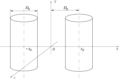
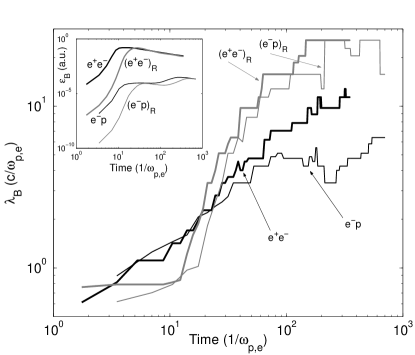
Figure 1.— A schematic representation of the initial state.

Figure 2.— Temporal evolution of the field correlation length in four scenarios. The subscript R denotes relativistic shells ($\mathbf{u}_{R}=\gamma\mathbf{v}=\pm 10.0\,c\,\hat{z}$, while $\mathbf{u}=\pm 0.6\,c\,\hat{z}$ otherwise, with $u_{\mathrm{th}}=\gamma v_{\mathrm{th}}=0.1c$). In the range $20/\omega_{p,e}<t<100/\omega_{p,e}$, $\lambda_{B}\propto t^{\alpha}$ with $\alpha=0.7,\,0.6,\,1,\,1.2$ for $e^{-}e^{+}$, $e^{-}p$, $(e^{-}e^{+})_{R}$, $(e^{-}p)_{R}$, respectively. In the inset, we show the evolution of the B-field equipartition parameter; note that at $20/\omega_{p,e}\lesssim t\lesssim 100/\omega_{p,e}$, $\epsilon_{B}\approx\mathrm{const.}$.

References

- Biskamp & Bremer (1994) Biskamp, D., & Bremer, U. 1994, Phys. Rev. Lett., 72, 3819
- Fonseca, et al. (2002) Fonseca, R. A., et al. 2002, Lecture Notes in Computer Science 2329, III-342 (Heidelberg: Springer-Verlag)
- Frederiksen, et al. (2004) Frederiksen, J. T., Hededal, C. B.; Haugblle, T., & Nordlund, Å2004, ApJ, 608, L13
- Kazimura, et al. (1998) Kazimura, Y., Sakai, J. I., Neubert, T., & Bulanov, S. V. 1998, ApJ, 498, L183
- Medvedev & Loeb (1999) Medvedev, M. V., & Loeb, A. 1999, ApJ, 526, 697
- Nishikawa, et al. (2003) Nishikawa, K.-I., Hardee, P., Richardson, G., Preece, R., Sol, H., & Fishman, G. J. 2003, ApJ, 595, 555
- Saito & Sakai (2004) Saito, S. & Sakai, J. I. 2004, ApJ, 604, L133
- Silva, et al. (2003) Silva, L. O., Fonseca, R. A., Tonge, J. W., Dawson, J. M., Mori, W. B., & Medvedev, M. V. 2003, ApJ, 596, L121