Observations of Magnetic Fields in the Milky Way and in Nearby Galaxies with a Square Kilometre Array
Abstract
The role of magnetic fields in the dynamical evolution of galaxies and of the interstellar medium (ISM) is not well understood, mainly because such fields are difficult to directly observe. Radio astronomy provides the best tools to measure magnetic fields: synchrotron radiation traces fields illuminated by cosmic-ray electrons, while Faraday rotation and Zeeman splitting allow us to detect fields in all kinds of astronomical plasmas, from lowest to highest densities. Here we describe how fundamental new advances in studying magnetic fields, both in our own Milky Way and in other nearby galaxies, can be made through observations with the proposed Square Kilometre Array. Underpinning much of what we propose is an all-sky survey of Faraday rotation, in which we will accumulate tens of millions of rotation measure measurements toward background radio sources. This will provide a unique database for studying magnetic fields in individual Galactic supernova remnants and H ii regions, for characterizing the overall magnetic geometry of our Galaxy’s disk and halo, and for understanding the structure and evolution of magnetic fields in galaxies. Also of considerable interest will be the mapping of diffuse polarized emission from the Milky Way in many narrow bands over a wide frequency range. This will allow us to carry out Faraday tomography of the Galaxy, yielding a high-resolution three-dimensional picture of the magnetic field within a few kpc of the Sun, and allowing us to understand its coupling to the other components of the ISM. Finally, direct synchrotron imaging of a large number of nearby galaxies, combined with Faraday rotation data, will allow us to determine the magnetic field structure in these sources, and to test both the dynamo and primordial field theories for field origin and amplification.
1 Introduction
A full understanding of galactic structure and evolution is impossible without understanding magnetic fields. Magnetic fields fill interstellar space, contribute significantly to the total pressure of interstellar gas, are essential for the onset of star formation, and control the density and distribution of cosmic rays in the interstellar medium (ISM). However, because magnetic fields cannot be directly observed, our understanding of their structure and origin lags significantly behind that of the other components of the ISM.
Radio astronomy has long led the way in studying astrophysical magnetic fields. Synchrotron emission measures the total field strength; its polarization yields the regular field’s orientation in the sky plane and also gives the field’s degree of ordering; Faraday rotation provides a measurement of the mean direction and strength of the field along the line of sight; the Zeeman effect provides an independent measure of field strength in cold gas clouds. All these effects have been effectively exploited. However, the study of magnetism in the Milky Way and in galaxies is a field still largely limited to examination of specific interesting regions, bright and nearby individual sources, and gross overall structure. Here we describe how exciting new insights into magnetic fields can be provided by the unique sensitivity, resolution and polarimetric capabilities of the Square Kilometre Array (SKA).
2 All-sky Rotation Measures
2.1 Background
While synchrotron emission and its polarization are useful tracers of magnetic fields, they are only easily detected in regions where the density of cosmic rays (i.e., relativistic gas) is relatively high, or where the magnetic field is strong. Many regions of interest for magnetic field studies are far from sites of active star formation and supernova activity, and thus cannot be studied through these techniques.
A much more pervasive probe of interstellar magnetic fields is Faraday rotation, in which birefringence in the magneto-ionic ISM causes the position angle of a linearly polarized wave to rotate. For a wave with emitted position angle observed at a wavelength , the detected position angle is:
| (1) |
In this expression, the rotation measure (RM), in units of rad m-2, is defined by :
| (2) |
where rad m-2 pc-1 cm3 G-1, , and are the regular magnetic field strength, inclination of the magnetic field to the line of sight and number density of thermal electrons, respectively, and the integral is along the line of sight from the observer to the source.
Multiwavelength observations of polarized sources can directly yield the RM along the line of sight. An estimate of RM in itself does not directly yield a value for , but the sign of the RM can provide information on the direction of the regular magnetic field. Furthermore, in cases where something is known about the electron density along the line of sight (e.g., from H observations, thermal radio emission, X-ray data, or pulsar dispersion measures), an estimate of the mean amplitude of the magnetic field strength along the line of sight can be directly inferred (a caveat is that correlations between and clumpiness in and both need to be properly accounted for in such estimates; [9]).
Thus provided that one can find a linearly polarized source as background, one can infer the strength and geometry of the magnetic field in foreground material, regardless of the foreground source’s synchrotron emissivity. However, for studying magnetic fields within the Galaxy, a serious shortcoming of this technique is the lack of background objects — for both pulsars and extragalactic radio sources, limited sky coverage and relatively poor sensitivity in polarization surveys severely limit the number of sightlines towards which one can measure the rotation measure in a foreground object, particularly if the source is of small angular extent (e.g., an H ii region or a supernova remnant). Until recently, there were only about 1200 RM measurements of compact sources over the entire sky (about 900 extragalactic sources, plus 300 pulsars), as shown in Figure 1. In the Galactic plane, new surveys are expanding this sample at a rate of about one RM measurement per deg2 (e.g., [35, 16]); over the rest of the sky, observations with the Effelsberg telescope of polarized NVSS sources will soon add another RM measurements. Such data sets are proving useful in studying the global properties of the Galactic magnetic field (e.g., [17]), but do not have a dense enough sampling for detailed modeling or for studying discrete foreground objects [43, 69].

2.2 A Survey for Polarized Sources with the SKA
An exciting experiment for the SKA will be to greatly increase the density of polarized background sources on the sky, providing enough statistics to make possible the study of all manner of foreground magneto-ionic sources. We thus propose an all-sky RM survey, which can provide a closely-packed grid of RM measurements in any direction. In the following discussion, we assume that the SKA has a sensitivity m2 K-1, of which 75% is distributed on baselines shorter than km, that the field of view at 1.4 GHz is 1 deg2, and that the total bandwidth available at 1.4 GHz is 25% (i.e., 350 MHz). If we aim to survey 10 000 deg2 of the sky in one year of integration time, the integration time per pointing is hour, and the expected sensitivity in linear polarization (i.e., from the combination in quadrature of Stokes and ) is then Jy. While a year of observing time is a large request, we note that such a survey has many other applications (e.g., Stokes imaging, H i absorption, pulsar surveys), and that it is reasonable to assume that multiple projects could piggyback on the same set of observations.
An important requirement for the SKA will be spectropolarimetric capability, wherein full Stokes products will be available in multiple contiguous channels across a broad continuum bandwidth. Provided that at least channels are available across the band, the individual channel widths determine the maximum value of which can be measured, while the total bandwidth determines the accuracy of the RM measurement. For an observing wavelength , a total bandwidth (in wavelength units) , and a source detected with signal to noise in linear polarization, the expected precision of an RM measurement is:
| (3) |
An appropriate observing wavelength for detecting large numbers of RMs is cm: this provides a large field of view, without introducing severe internal depolarization effects which will prevent RMs from being measured in many extragalactic background sources. At 21 cm, our assumed fractional bandwidth of 25% corresponds to . For a precision in RM of rad m-2, we thus require a signal to noise in polarization . (Such a precision in RM is more than sufficient for the purposes considered here; higher precision measurements are possible, but require correction for the effects of the Earth’s ionosphere.)
Given the high density of polarized sources expected on the sky (see below), we require an angular resolution to ensure that the polarized sky is not confusion limited. To carry out an efficient survey, we will need to image the full 1-deg2 field of view of the SKA at this resolution. If this field corresponds to the primary beam of a single element, then individual channel widths need to be smaller than kHz to avoid bandwidth smearing (i.e., channels will be needed across the 25% observing bandwidth). This also is more than sufficient to completely mitigate bandwidth depolarization provided rad m-2, which is likely to be the case for almost all sightlines. Low values of can be directly identified from images of linear polarization using just a few (10) channels across the observing bandwidth and fitting directly to the position angle swing across this band [35]; the polarized signal from high-RM sources will require Fourier analysis of the polarimetric signal to identify [18, 48], but ultimately can be recovered with the same signal-to-noise as for the low-RM case.
We conclude our description of this experiment by noting its implications for polarization purity and for imaging dynamic range. As discussed in the following section, the peak in the distribution of fractional polarization for extragalactic sources is expected to be at (where is the fractional linear polarization), but with a significant fraction of the population extending down to . Thus in order to be able to detect polarization in the bulk of sources, the final calibrated mosaiced images require a polarization purity of at least –25 dB over the entire field. We assume that the final images will incorporate averaging of overlapping fields and wide parallactic angle coverage, which will assist in achieving this target. We note that a higher polarization purity, closer to –40 dB, is required for single-pointing on-axis observations, for which experiments involving very weakly polarized sources may be important.
The density of polarized sources shown in Figure 2 implies that in any 1-deg2 field, we always expect to detect at least one source whose linearly polarized flux density is mJy. Thus to detect polarized sources as faint as 1 Jy (the 10- detection limit of a 1-hour integration) a modest dynamic range of at least 6000 is required. We note also that in this same field, we expect to detect at least one source whose total intensity is mJy. For a polarization purity no worse than –25 dB anywhere in the field, this will result in leakage into the polarized image at the level of 0.6 mJy; this should not present any challenges to obtaining high dynamic range in the polarized images.
2.3 Detection Statistics for the SKA RM Survey
We first consider the likely detection statistics for pulsars. The polarimetry statistics of Gould & Lyne [36] suggest that pulsars have a typical linearly polarized fraction of %. Thus the faintest pulsar from which we can extract a useful RM measurement will have a total intensity flux density of Jy. This is sufficient to detect virtually every radio pulsar in the Galaxy which is beaming towards us [49], i.e. about 20 000 pulsars. We assume that most of these pulsars lie at Galactic latitudes , so that the area of the sky under consideration is 3600 deg2. Thus the expected source density of RMs from pulsars is about 6 deg-2, or an angular spacing of about one source every in the Galactic plane.
For extragalactic background sources, we can estimate the likely distribution of polarized sources by convolving the differential source count distribution, , by the probability distribution of fractional polarized intensity, . can be obtained directly from deep continuum surveys and extrapolations thereof [44, 45, 65], while can be estimated from the 1.4 GHz NVSS catalog [23]. Considering only NVSS sources with flux densities mJy so as to eliminate most sources whose polarized fraction is below the sensitivity of the survey, we find that can be fitted by two Gaussian components, centered at . In the following discussion we assume that this distribution of does not evolve as a function of flux density, although we note that several recent studies have suggested that weaker sources are more highly polarized [56, 77, 78]. If this effect is real, our source count estimates should be considered a lower limit.
Convolving with results in a predicted linearly polarized differential source count distribution as shown in Figure 2. Down to a flux limit of Jy, we thus expect a density of polarized sources of deg-2. Only about 50% of these sources will have measurable RMs, usually due to internal depolarization which destroys the RM dependence predicted from Equation (1) [16]. We thus expect to find RMs over the survey (about one RM per second of observing time!), at a mean separation of between adjacent measurements. For particular regions of interest (e.g., towards a specific supernova remnant or nearby galaxy), one could carry out a much deeper integration to further improve the spacing of this “RM grid”. For example, in a 10-hour targeted observation, the mean spacing of RM measurements would shrink to .

3 Scientific Applications of an RM Grid
The densely-spaced RM grid which would result from the experiment proposed above will have numerous applications: the magnetic properties of any extended foreground object will be able to be mapped in detail. Before discussing specific projects, we make a few general comments about such analyses:
-
•
The RM signature of an extended foreground object can only ever be identified provided that its contribution to the total RM dominates the average intrinsic RM of the background sources. Since the intrinsic RM of extragalactic sources, averaged over many such objects, is rad m-2, we should be easily able to identify the extra RM signal produced by intervening supernova remnants (SNRs) and H ii regions, or by diffuse magnetic fields in the Milky Way, in other galaxies or in galaxy clusters.
-
•
A RM only probes the line-of-sight component of an object’s regular magnetic field. For studies of individual objects, full three-dimensional geometries can be inferred by combining such measurements with other probes: e.g., linear polarization position angles of synchrotron emission for SNRs, infrared polarimetry for H ii regions, or depolarization effects (e.g., [29]). However, for studies of an ensemble of objects, or of turbulent processes, the RM measurements alone can suffice. We also note that thanks to our position within the Milky Way, the three-dimensional field geometry can be inferred by considering RM properties in different parts of the sky, since each RM probes the parallel field component in a different direction. This method is also applicable to nearby galaxies which are significantly inclined with respect to the line of sight [29].
-
•
While pulsars have a much lower source density than extragalactic sources, all pulsars will also have measurements of their dispersion measure (DM). Dividing the RM by the DM can allow a direct estimate of the mean magnetic field strength along the line of sight, subject to caveats on possible correlations between the magnetic field strength and the electron density [9]. For nearby pulsars, distances will be directly available from parallax measurements [19]; for more distant sources the distance can be estimated from the DM [24].
3.1 The Milky Way
Our own Galaxy provides a wonderful opportunity for a detailed study of the generation and amplification of galactic magnetic fields, and their coupling to the ISM. However, we currently lack a good understanding of the overall field geometry, including the number and location of reversals, the pitch angle of the presumed spiral pattern of the disk’s magnetic field, and the structure of the magnetic field in the halo [6]. This results both from the sparse sampling of RMs, and from the lack of sensitivity to pulsars in the more distant parts of the Galaxy.
The SKA RM survey proposed above will overcome all these limitations. Using wavelet transforms, the Galactic pulsar RM distribution can be directly inverted to delineate the full geometry of the Galactic magnetic field in the disk (Fig. 3). Extragalactic RMs can trace components of the magnetic field such as the outer arms [17] and the vertical structure of the field in the disk and halo [38], and can also identify loops and other features which trace Galactic structure (e.g., [67]).
The RM grid will also be a powerful probe of turbulence. Turbulence is thought to be injected at specific size scales into the ISM by various processes, and then cascades down to increasingly smaller scales before ultimately being dissipated as heat. It has been argued that the amplitudes of turbulent fluctuations in the ISM form a single power spectrum extending from the largest Galactic scales ( 1 kpc) down to a tiny fraction of an AU [2]. However, there are observational indications that the slope of the power spectrum may deviate from that predicted by the standard three-dimensional Kolmogorov model for the cascade (e.g., [58, 74]). Futhermore, it is likely that the turbulent properties of the ISM strongly depend on location within the Galaxy, as might be expected if SNRs or H ii regions are responsible for providing much of the energy which goes into turbulent motions (e.g., [42]). Finally, our understanding of how fluctuations in magnetic field strength couple to those in electron density is still limited (e.g., [54, 21]).
An ensemble of polarized extragalactic background sources can be used to compute structure functions, wavelet transforms and autocorrelation functions of RM (e.g., [52, 58, 32, 28]), all of which provide different information on the combined spatial power spectrum of density and magnetic field fluctuations in ionised gas. However, the sparse sampling of current data sets prevents a detailed analysis on scales much smaller than a degree. With the SKA, the dense grid of RM measurements can allow computation of virtually continuous power spectra of RM, on scales ranging from up to tens of degrees. This will allow a full characterization of magneto-ionic turbulence in this range of angular scales.111SKA experiments relating to ISM turbulence on much smaller scales are discussed in Lazio et al., this volume. We will also be able to generate such power spectra as a function of Galactic longitude and latitude, so as to establish how the turbulent properties of the ionised ISM vary, e.g., between arm and inter-arm regions, between star-forming and quiescent regions, or between the thin disk, the thick disk and the halo.
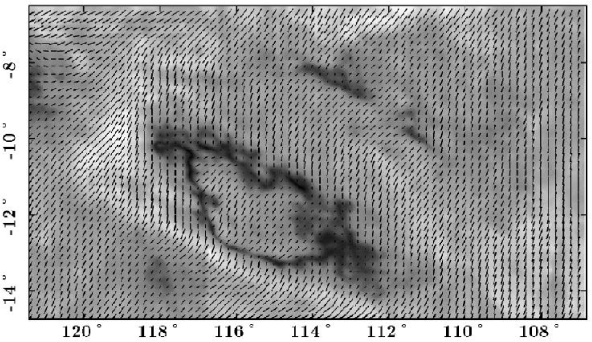
An additional resource will be the diffuse polarization seen all over the sky, such as is shown in Figure 4. In such fields the RM can be measured at every pixel, allowing one to compute power spectra at even higher spatial resolutions than made possible by the RM grid of background sources [28, 42]. Such analyses are highly complementary to those toward the RM grid, because they probe a smaller sightline through the Galaxy, and thus give information on structure in specific local regions (see further discussion in §4).
At high latitudes, where optical extinction is minimal, the RMs of background sources can be directly compared to the H emission from diffuse ionised gas and to the DMs of pulsars in globular clusters, to separately solve for the mean electron density, gas clumping factor, magnetic field strength and direction, and the fluctuations in each of these quantities.
3.2 Galactic Supernova Remnants
Magnetic fields in SNRs are a key diagnostic of the physical processes which govern heating, turbulence and particle acceleration generated by strong shocks. Magnetic field strengths in SNR shocks are typically thought to be at the level of 1mG [33], but it is unclear how these high magnetic fields are produced, especially in young adiabatic SNRs where the compression ratio is small. Turbulent amplification in Rayleigh-Taylor unstable regions between the forward and reverse shocks of the SNR can generate strong magnetic fields [46, 47]. This may in turn result in significant second-order Fermi acceleration of cosmic rays, and could have an important bearing on the overall evolution of SNRs [60, 34].
With current data we are unable to address these issues. While the position angle of polarized emission provides the orientation of the magnetic field [57, 33], we normally do not have a good estimate of the field strength in these regions, because there is little reason to assume that magnetic fields and cosmic rays are in equipartition. Only in a few sources can we directly infer the magnetic field strength via Zeeman splitting of shock-excited OH masers [15], but these are likely to be special cases where the shock is radiative and is interacting with a molecular cloud [20]. Once again, the RM grid provides the potential to directly measure magnetic fields on small scales in these sources. Specifically, one can combine RM measurements with observations of thermal X-rays from SNR shocks, to separate out density and magnetic field contributions to the RM [55]. With the SKA, this technique can be applied to many SNRs, embedded in many different environments, and at a wide range of evolutionary stages.
A related experiment corresponds to the effect that SNRs should have on their surroundings. It is widely believed that SNRs accelerate cosmic rays through diffusive shock acceleration. An important part of this process is that particles streaming away from the shock generate enhanced magnetohydrodynamic turbulence just upstream, which in turn provides the scattering centers which reflect particles back across the shock (e.g., [1]). Because of this process, it is reasonable to suppose that SNR shocks inject significant amounts of turbulent energy into their surroundings, which ultimately become part of the overall turbulent cascade. These physical processes can be directly tested by observations of RMs of background sources, in that we expect to see enhanced amplitudes and dispersions of RMs immediately beyond the bright radio rims of young SNRs. A preliminary effort in this regard tentatively suggests that indeed there is a larger scatter in the RMs of sources behind SNRs than in other regions [68], but from the crude statistics of that study it is difficult to disentangle the effect of a SNR itself from the complicated environment in which it is often embedded. The much denser sampling which the SKA will generate, accumulated over many SNRs in the Galactic plane, can provide a definitive study of this effect.
Finally, it is thought that in many cases (most notably around the Crab Nebula), the SNR shock is invisible, perhaps because it has not yet interacted significantly with the ISM (e.g., [30]). Such shocks might be detectable by their effect on the RMs of background sources; such a detection would greatly add to our understanding of the evolution of young SNRs expanding into low density regions or into stellar wind bubbles.
3.3 Galactic H ii Regions
H ii regions provide a link between the molecular clouds from which stars form, the powerful winds which massive stars generate, and the ambient ISM into which all this material ultimately diffuses. Because H ii regions span a very wide range of densities, studies of magnetic fields in H ii regions provide an insight into how magnetic fields control the flow of gas, and conversely how compression of gas can amplify magnetic fields [76]. Zeeman splitting of masers can probe magnetic fields in ultracompact H ii regions, but it is difficult to measure magnetic fields in more diffuse sources. Heiles & Chu [43] demonstrated that RMs of background sources can yield such measurements, but until now this technique has had limited application because of the sparseness of such background sources. With the SKA, the RM produced by H ii regions can be probed in detail using such background sources; since electron densities are readily determined from H or radio continuum observations, the magnetic field strength can be easily extracted from the RM [35]. With these data we can characterize how gas and magnetic fields are compressed by ionization fronts, how the ionization fraction within photo-dissociation regions varies with distance from the central star, and what role magnetism plays in the highly turbulent interiors of H ii regions.
Finally, we note that since RM signals from low density ionized regions are much more easily identified than emission measures or other tracers, many groups are now identifying unusual regions of ionised gas which are only seen by their effect on the diffuse polarized emission of the Galactic background (Fig. 4; [37, 41]). With the wide field of view of the SKA, we expect to be able to identify many more such sources. The continuous frequency coverage of these observations will allow detailed tomographic studies (see §4), which can allow us to better establish these sources’ basic properties.
3.4 Nearby Galaxies
Magnetic fields can be detected via synchrotron emission only if there are cosmic-ray electrons to illuminate them. Cosmic rays are probably accelerated in objects related to star formation. However, the radial scale length of synchrotron emission in nearby galaxies is much larger than that of the star formation indicators like infrared or CO line emission [7]. Magnetic fields must extend to very large radii, much beyond the star-forming disk. In the outermost parts of galaxies the magnetic field energy density may even reach the level of global rotational gas motion and affect the rotation curve [3].
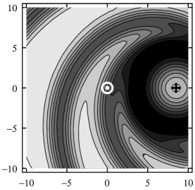
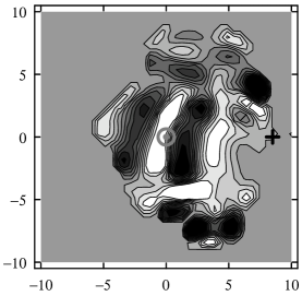
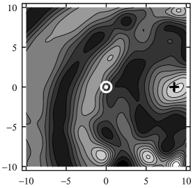
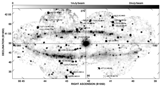
Field strengths in the outer parts of galaxies can only be measured by Faraday rotation measures of polarized background sources. Han et al. [39] found evidence for regular fields in M 31 at 25 kpc radius of similar strength and structure as in the inner disk. However, even within the huge field of M 31 observed with the VLA (B array) at 1.4 and 1.7 GHz, only 21 sources with sufficient polarization flux densities were available (Fig. 5). With only a few detectable polarized sources per square degree at current sensitivities (see Fig. 2), no galaxies beyond M 31 can be mapped in this way.
The SKA will dramatically improve the situation. Within the fields of M 31, the LMC or the SMC (a few square degrees each), a deep observation could provide polarized background sources, and thus allow fantastically detailed maps of the magnetic structure. The field of a spiral galaxy at 10 Mpc distance will still include about 50 sources; several hundred galaxies could be studied in this way.
The sensitivity of the rotation measure maps obtained by smoothing of the RM grid will be better than 1 rad m-2, allowing us to detect fields weaker than G in a halo of cm-3 electron density, or ionised gas of less than cm-3 electron density in a 5 G regular field (assuming a pathlength of 1 kpc for both cases). The SKA will be by far the most sensitive detector of magnetic fields and ionised gas in the outskirts of galaxies and in the intergalactic medium.
4 Faraday Tomography
Major progress in detecting small structures has recently been achieved with decimetre-wave polarization observations in the Milky Way [26, 27, 35, 40, 41, 62, 79, 80, 81]. A wealth of structures on parsec scales has been discovered: filaments, canals, lenses, and rings (e.g., Fig. 4). Their common property is that they appear only in maps of polarized intensity, but not in total intensity. Some of these features directly trace small-scale structures in the magnetic fields or ionised gas. Other features are artifacts due to Faraday rotation (Faraday ghosts) and may give us new information about the properties of the turbulent interstellar medium [64]. To distinguish and interpret these phenomena, a multifrequency approach has to be developed.
At the low frequencies of these polarization surveys, strong Faraday depolarization occurs both in regions of regular field (differential Faraday rotation) and in those of random fields (Faraday dispersion) [71]. The effect of Faraday depolarization is that the ISM is not transparent to polarized radio waves; the opacity varies strongly with frequency and position on sky. For Faraday dispersion the observable depth can be described by an exponentially decreasing function. At low frequencies only emission from nearby regions can be detected. In the local ISM, the typical observation depth is kpc around 5 GHz, 1–5 kpc around 1 GHz, and pc around 0.3 GHz. Different frequencies trace different layers of polarized emission; we call this new method Faraday tomography. Individual field structures along the line of sight can be isolated, either by their polarized synchrotron emission, by Faraday rotation or by Faraday depolarization of the diffuse emission from the Galactic background. The distances to these polarized structures can be determined by measuring the H i absorption to these features in Stokes and [25]. With a large number of channels, “RM synthesis” becomes possible [18, 48], where the channel width determines the observable RM range and the total frequency range determines the half-power width of the “RM visibility function”. This method also allows us to distinguish emitting regions at different distances along the same line of sight through their different RMs. This tomography database can be used to study the properties of magneto-ionic turbulence in the ISM by calculating the structure function or wavelet transforms of the three-dimensional structure in polarized intensity and RM (a few two-dimensional studies of limited areas have already been carried out [74, 42]).
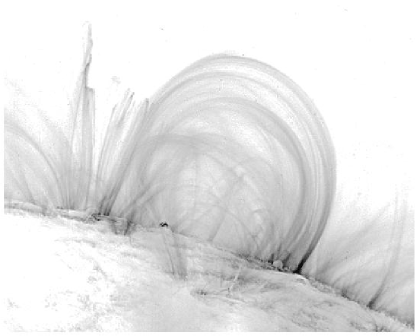
Present-day radio polarization observations reveal only unsharp images of magnetic fields in the ISM. The high resolution of the SKA will show field structures illuminating the dynamical interplay of cosmic forces [61]: loops, twisted fibres, and field reversals, as observed on the Sun (Fig. 6). The widths of such structures can be in the range 0.1–1 pc, but are probably larger in irregular and dwarf galaxies. With a regular field strength of 30 G (in equipartition with cosmic rays) and 1 pc extent along the line of sight, a (distance-independent) polarization surface brightness at 5 GHz of 0.2 Jy per beam is expected. The SKA will be able to detect such features in the Magellanic Clouds ( = 0.24 pc) and in M 31 / M 33 ( = 3.5 pc) within a few hours. In the Milky Way they are hard to detect among many other emitters along the line of sight, but Faraday tomography can isolate them.
Bright synchrotron filaments have been detected near the Galactic Centre with milligauss field strengths [59]. In the “Arc” and the “Snake”, particle acceleration probably occurs in reconnection regions [11, 53]. Magnetic reconnection may be a common process in the ISM and an important heating source also in galaxy halos [12], but only the most prominent regions in the Milky Way are visible with present-day telescopes. Acceleration of cosmic rays should produce strong synchrotron emission in a small volume. Even a relatively weak regular field of strength 50 G with 1 pc extent, in equipartition with cosmic rays, generates emission with a polarization surface brightness at 5 GHz of 1.5 Jy per beam which clearly emerges above the background. Field reversals across reconnection regions should also be detectable via rotation measures.
The angular resolution of the SKA will allow us to trace directly how interstellar magnetic fields are connected to gas clouds. The close correlation between radio continuum and mid-infrared intensities within galaxies [31] indicates that a significant fraction of the magnetic flux is connected to gas clouds. Photo-ionisation may provide sufficient density of thermal electrons in the outer regions of gas clouds to hold the field lines. Observational support comes from the detection of Faraday screens in front of a molecular cloud in the Taurus complex in our Galaxy [82]. As no enhanced H emission has been detected in this direction, the local field enhancement must be significant. Faraday tomography with the SKA will allow to detect such Faraday screens toward molecular clouds throughout the Milky Way and in nearby galaxies. A SKA beam resolves 3.5 pc in M 31 where clouds at various evolutionary stages are available. SKA will allow to trace these and contribute to solving the puzzle of star formation.
It is essential that the frequencies of Faraday tomography observations are distributed continuously over a broad bandwidth. The frequency range has to be chosen according to the strengths of the regular and random fields, the electron density and the pathlength through the Faraday-rotating region. The RM grid (see §2) helps choose the best frequencies. To cover a wide range of physical parameters, the SKA has to operate in the frequency range of at least 0.5–10 GHz, but 0.3–20 GHz is desirable. Sensitive imaging of extended structures requires that most of the collecting area lies on baselines shorter than 100 km.
5 Dynamo versus Primordial Field Origin
The observation of large-scale patterns in RM in many galaxies [5] proves that the regular field in galaxies has a coherent direction and hence is not generated by compression or stretching of irregular fields in gas flows. In principle, the dynamo mechanism is able to generate and preserve coherent magnetic fields, and they are of appropriate spiral shape [8] with radially decreasing pitch angles [4]. However, the physics of dynamo action is far from being understood and faces several theoretical problems [14, 51]. Primordial fields, on the other hand, are hard to preserve over a galaxy’s lifetime due to diffusion and reconnection because differential rotation winds them up. Even if they survive, they can create only specific field patterns that differ from those observed [66, 70].
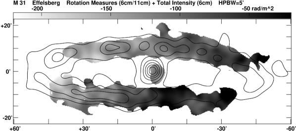
The widely studied mean-field – dynamo model needs differential rotation and the effect (see below). Any coherent magnetic field can be represented as a superposition of modes of different azimuthal and vertical symmetries. The existing dynamo models predict that several azimuthal modes can be excited [8], the strongest being (an axisymmetric spiral field), followed by the weaker (a bisymmetric spiral field), etc. These generate a Fourier spectrum of azimuthal RM patterns. The axisymmetric mode with even vertical symmetry (quadrupole) is excited most easily. Primordial field models predict bisymmetric fields or axisymmetric fields with odd (dipole) symmetry [70]. For most of about 20 nearby galaxies observed so far, the RM data indicate a mixture of magnetic modes which cannot be reliably determined due to low angular resolution and/or low signal-to-noise ratios [5]. M 31 is an exception with a strongly dominating axisymmetric field (Fig. 7).
The SKA will be able to confidently determine the Fourier spectrum of dynamo modes. To detect an azimuthal mode of order , the spatial resolution has to be better than where is the galaxy’s radius. With and kpc a spatial resolution of 0.2 kpc is needed which is presently available (with sufficient sensitivity) only for galaxies in the Local Group.
Typical polarization intensities of nearby galaxies at 5 GHz are 0.1 mJy per beam. Within a beam, 0.4 Jy is expected, which the SKA can detect in hour of integration. Hence, the SKA can resolve all modes up to in galaxies out to a distance of 40 Mpc. The RM grid discussed in §2 can identify the best candidates.
The SKA has the potential to increase the galaxy sample with well-known field patterns by up to three orders of magnitude. The conditions for the excitation of dynamo modes can be clarified. For example, strong density waves are claimed to support the mode while companions and interactions may enhance the bisymmetric mode. A dominance of bisymmetric fields over axisymmetric ones would be in conflict with existing dynamo models and would perhaps support the primordial field origin [70].
Dynamo models predict the preferred generation of quadrupolar patterns in the disk where the field has the same sign above and below the plane, while the field may be dipolar in the halo ([8]). Primordial models predict dipolar patterns in the disk and in the halo with a reversal in the plane [70], which can be distinguished using RMs in edge-on galaxies. However, the polarized emission from radio halos is weak so that no single determination of the vertical field symmetry has been possible yet. This experiment also must await the SKA.
The all-sky RM grid will allow us to trace coherent fields to large galactic radii, well beyond the regions in which star formation takes place, and to derive restrictions for the effect. This is an essential ingredient of dynamo action and describes the mean helicity of turbulent gas motions. If the effect is driven by supernova remnants or by Parker loops, dynamo modes should be excited preferably in the star-forming regions of a galaxy. But if the magneto-rotational (Balbus-Hawley) instability is the source of turbulence and of the effect [63], magnetic field amplification with some fraction of regular fields will be seen out to large galactic radii.
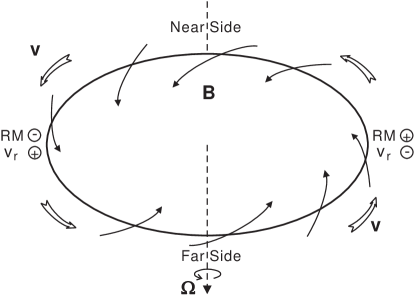
The few galaxies known to host a dominating axisymmetric mode possess a radial field component which is directed inwards everywhere [50]. As the field direction in dynamo models is arbitrary, it preserves the memory of the seed field which may be a regular primordial field with a preferred direction. The sign of the field component along radius follows from observations of Faraday rotation (RM) and of rotational velocity along the line of sight () on both sides of the galaxy’s major axis (Fig. 8): opposite signs of RM and indicate an inward-directed field, while the same signs an outward-directed field. SKA’s sensitivity will allow to observe a large galaxy sample (a beam will let us study such sources out to 100 Mpc) and will clearly show any preferred field direction.
The lack of a coherent magnetic field in a resolved galaxy would indicate that the timescale for dynamo action is longer than the galaxy’s age, or that the mean-field dynamo does not work at all. The role of the dynamo may still be important for the transformation of turbulent kinetic energy into magnetic energy (the fluctuation dynamo [13, 73]). Unlike the mean-field dynamo discussed above, the fluctuation dynamo amplifies and maintains only turbulent, incoherent magnetic fields and does not rely on overall differential rotation and the effect. This process seems to work in all types of galaxies as long as their star formation activity is sufficiently high. For example, dwarf irregular galaxies with almost chaotic rotation host turbulent fields with strengths comparable to spiral galaxies, but have no large-scale coherent fields [22].
6 Summary
A 1.4-GHz all-sky survey of Faraday rotation will accumulate tens of millions of rotation measure measurements toward background radio sources. This will allow us to characterize the overall magnetic geometry and turbulent properties of the disk and halo of the Milky Way, and of embedded individual objects such as H ii regions and supernova remnants. In a highly complementary fashion, mapping of diffuse polarized emission from the Milky Way in many narrow bands over a wide frequency range will allow us to carry out Faraday tomography of the local Galaxy. The observing frequency for this tomography needs to be tuned to the ISM properties under study, e.g., GHz for low-density regions and GHz for high-density regions. The combination of these observations will yield a high-resolution three-dimensional picture of the magnetic field within a few kpc of the Sun. Direct synchrotron imaging of a large number of nearby galaxies (at frequencies GHz where Faraday depolarization is minimal) will uncover the detailed magnetic field structure in these sources. Together with Faraday rotation data from diffuse emission and from the all-sky survey of background sources, we will be able to test both the dynamo and primordial field theories for field origin and amplification and hence can establish an understanding of the structure and evolution of magnetic fields in galaxies.
We thank Andrew Hopkins and Nick Seymour for providing information on source count distributions, Jo-Anne Brown for supplying Figure 1, and Wolfgang Reich for Figure 4. We also thank Elly Berkhuijsen, Marijke Haverkorn, John Dickey, Wolfgang Reich and Anvar Shukurov for many useful comments. B.M.G. acknowledges the support of the National Science Foundation through grant AST-0307358. The Transition Region and Coronal Explorer (TRACE), is a mission of the Stanford-Lockheed Institute for Space Research, and part of the NASA Small Explorer program. The National Radio Astronomy Observatory is a facility of the National Science Foundation operated under cooperative agreement by Associated Universities, Inc.
References
- [1] Achterberg, A., Blandford, R. D., Reynolds, S. P., 1994, A&A, 281, 220
- [2] Armstrong, J. W., Rickett, B. J., Spangler, S. R., 1995, ApJ, 443, 209
- [3] Battaner, E., Florido, E., 2000, Fund. Cosmic Phys., 21, 1
- [4] Beck, R., 1993, in The Cosmic Dynamo, eds. F. Krause et al., Kluwer, Dordrecht, p. 283
- [5] Beck, R., 2000, Phil. Trans. R. Soc. Lond. A, 358, 777
- [6] Beck, R., 2001, Sp. Sci. Rev., 99, 243
- [7] Beck, R., 2004, Astrophys. Sp. Sci., 289, 293
- [8] Beck, R., Brandenburg, A., Moss, D., Shukurov, A., Sokoloff, D., 1996, ARA&A, 34, 155
- [9] Beck, R., Shukurov, A., Sokoloff, D., Wielebinski, R., 2003, A&A, 411, 99
- [10] Berkhuijsen, E. M., Beck, R., Hoernes, P., 2003, A&A, 398, 937
- [11] Bicknell, G. V., Li, J., 2001, ApJ, 548, L69
- [12] Birk, G. T., Lesch, H., Neukirch, T., 1998, MNRAS, 296, 165
- [13] Blackman, E. G., 1998, ApJ, 496, L17
- [14] Brandenburg, A., Subramanian, K., 2004, Phys. Rep., in press, astro-ph/0405052
- [15] Brogan, C. L., Frail, D. A., Goss, W. M., Troland, T. H., 2000, ApJ, 537, 875
- [16] Brown, J. C., Taylor, A. R., Jackel, B. J., 2003, ApJS, 145, 213
- [17] Brown, J. C., Taylor, A. R., Wielebinski, R., Müller, P., 2003, ApJ, 592, L29
- [18] de Bruyn, A. G., 1996, NFRA Note 655
- [19] Chatterjee, S., Cordes, J. M., Vlemmings, W. H. T., Arzoumanian, Z., Goss, W. M., Lazio, T. J. W., 2004, ApJ, 604, 339
- [20] Chevalier, R. A., 1999, ApJ, 511, 798
- [21] Cho, J., Lazarian, A., 2003, MNRAS, 345, 325
- [22] Chyży, K. T., Knapik, J., Bomans, D. J., Klein, U., Beck, R., Soida, M., Urbanik, M., 2003, A&A, 405, 513
- [23] Condon, J. J., Cotton, W. D., Greisen, E. W., Yin, Q. F., Perley, R. A., Taylor, G. B., Broderick, J. J., 1998, AJ, 115, 1693
- [24] Cordes, J. M., Lazio, T. J. W., 2002, preprint (astro-ph/0207156)
- [25] Dickey, J. M., 1997, ApJ, 488, 258
- [26] Duncan, A. R., Haynes, R. F., Jones, K. L., Stewart, R. T., 1997, MNRAS, 291, 279
- [27] Duncan, A. R., Reich, P., Reich, W., Fürst, E., 1999, A&A, 350, 447
- [28] Enßlin, T. A., Vogt, C., 2003, A&A, 401, 835
- [29] Fletcher, A., Berkhuijsen, E. M., Beck, R., Shukurov, A., 2004, A&A, 414, 53
- [30] Frail, D. A., Kassim, N. E., Cornwell, T. J., Goss, W. M., 1995, ApJ, 454, L129
- [31] Frick, P., Beck, R., Berkhuijsen, E. M., Patrickeyev, I., 2001, MNRAS, 327, 1145
- [32] Frick, P., Stepanov, R., Shukurov, A., Sokoloff, D., 2001, MNRAS, 325, 649
- [33] Fürst, E., Reich, W., 2004, in The Magnetized Interstellar Medium, eds. B. Uyanıker et al., p. 141
- [34] Gaensler, B. M., Wallace, B. J., 2003, ApJ, 594, 326
- [35] Gaensler, B. M., Dickey, J. M., McClure-Griffiths, N. M., Green, A. J., Wieringa, M. H., Haynes, R. F., 2001, ApJ, 549, 959
- [36] Gould, D. M., Lyne, A. G., 1998, MNRAS, 301, 235
- [37] Gray, A. D., Landecker, T. L., Dewdney, P. E., Taylor, A. R., 1998, Nature, 393, 660
- [38] Han, J. L., Manchester, R. N., Berkhuijsen, E. M., Beck, R., 1997, A&A, 322, 98
- [39] Han, J. L., Beck, R., Berkhuijsen, E. M., 1998, A&A, 335, 1117
- [40] Haverkorn, M., Katgert, P., de Bruyn, A. G., 2003a, A&A, 403, 1031
- [41] Haverkorn, M., Katgert, P., de Bruyn, A. G., 2003b, A&A, 404, 233
- [42] Haverkorn, M., Gaensler, B. M., McClure-Griffiths, N. M., Dickey, J. M., Green, A. J., 2004, ApJ, 609, 776
- [43] Heiles, C., Chu, Y.-H., 1980, ApJ, 235, L105
- [44] Hopkins, A. M., Windhorst, R., Cram, L. E., Ekers, R. D., 2000, Experimental Astronomy, 10, 419
- [45] Hopkins, A. M., Afonso, J., Chan, B., Cram, L. E., Georgakakis, A., Mobasher, B., 2003, AJ, 125, 465
- [46] Jun, B.-I., Norman, M. L., 1996, ApJ, 465, 800
- [47] Jun, B.-I., Norman, M. L., 1996, ApJ, 472, 245
- [48] Killeen, N. E. B., Fluke, C. J., Zhao, J.-H., Ekers, R. D., 2004, MNRAS, submitted (http://www.atnf.csiro.au/~nkilleen/rm.ps)
- [49] Kramer, M., 2003, in The Scientific Promise of the Square Kilometre Array, eds. M. Kramer & S. Rawlings, p. 85 (astro-ph/0306456)
- [50] Krause, F., Beck, R., 1998, A&A, 335, 789
- [51] Kulsrud, R. M., 1999, ARA&A, 37, 37
- [52] Lazio, T. J., Spangler, S. R., Cordes, J. M., 1990, ApJ, 363, 515
- [53] Lesch, H., Reich, W., 1992, A&A, 264, 493
- [54] Maron, J., Goldreich, P., 2001, ApJ, 554, 1175
- [55] Matsui, Y., Long, K. S., Dickel, J. R., Greisen, E. W., 1984, ApJ, 287, 295
- [56] Mesa, D., Baccigalupi, C., De Zotti, G., Gregorini, L., Mack, K.-H., Vigotti, M., Klein, U., 2002, A&A, 396, 463
- [57] Milne, D. K., 1990, in Galactic and Intergalactic Magnetic Fields, eds. R. Beck et al., Kluwer, Dordrecht, p. 67
- [58] Minter, A. H., Spangler, S. R., 1996, ApJ, 458, 194
- [59] Morris, M., 1996, in Unsolved Problems of the Milky Way, eds. L. Blitz & P. Teuben, Kluwer, Dordrecht, p. 247
- [60] Ostrowski, M., 1999, A&A, 345, 256
- [61] Parker, E. N., 1987, ApJ, 318, 876
- [62] Reich, W., Fürst, E., Reich, P., Uyanıker, B., Wielebinski, R., Wolleben, M., 2004, in The Magnetized Interstellar Medium, eds. B. Uyanıker et al., p. 45
- [63] Sellwood, J. A., Balbus, S. A., 1999, ApJ, 511, 660
- [64] Shukurov, A., Berkhuijsen, E. M., 2003, MNRAS, 342, 496, and MNRAS, 345, 1392 (Erratum)
- [65] Seymour, N., McHardy, I. M., Gunn, K. F., 2004, MNRAS, 352, 131
- [66] Shukurov, A., 2000, in The Interstellar Medium in M 31 and M 33, eds. E. M. Berkhuijsen et al., Shaker, Aachen, p. 191
- [67] Simard-Normandin, M., Kronberg, P. P., 1980, ApJ, 242, 74
- [68] Simonetti, J., 1992, ApJ, 386, 170
- [69] Simonetti, J. H., Cordes, J. M., 1986, ApJ, 303, 659
- [70] Sofue, Y., Fujimoto, M., Wielebinski, R., 1986, ARA&A, 24, 459
- [71] Sokoloff, D. D., Bykov, A. A., Shukurov, A., Berkhuijsen, E. M., Beck, R., Poezd, A.D., 1998, MNRAS, 299, 189, and MNRAS, 303, 207 (Erratum)
- [72] Stepanov, R., Frick, P., Shukurov, A., Sokoloff, D. D., 2002, A&A, 391, 361
- [73] Subramanian, K., 1998, MNRAS, 294, 718
- [74] Sun, X. H., Han, J. L., 2004, in The Magnetized Interstellar Medium, eds. B. Uyanıker et al., p. 25 (astro-ph/0402180)
- [75] Taylor, J. H., Manchester, R. N., Lyne, A. G., 1993, ApJS, 88, 529
- [76] Troland, T. H., Heiles, C., 1986, ApJ, 301, 339
- [77] Tucci, M., Martínez-González, E., Toffolatti, L., González-Nuevo, J., de Zotti, G., 2003, New Astronomy Reviews, 47, 1135
- [78] Tucci, M., Martínez-González, E., Toffolatti, L., González-Nuevo, J., De Zotti, G., 2004, MNRAS, 349, 1267
- [79] Uyanıker, B., Fürst, E., Reich, W., Reich, P., Wielebinski, R., 1998, A&AS, 132, 401
- [80] Uyanıker, B., Fürst, E., Reich, W., Reich, P., Wielebinski, R., 1999, A&AS, 138, 31
- [81] Uyanıker, B., Landecker, T. L., Gray A. D., Kothes, R., 2003, ApJ, 585, 785
- [82] Wolleben, M., Reich, W., 2004, in The Magnetized Interstellar Medium, eds. B. Uyanıker et al., p. 99