Relic gravitational waves and present accelerated expansion

Abstract

We calculate the current power spectrum of the gravitational waves created at the big bang (and later amplified by the different transitions during the Universe expansion) taking into account the present stage of accelerated expansion. Likewise, we determine the power spectrum in a hypothetical second dust era that would follow the present one if at some future time the dark energy, that supposedly drives the current accelerated expansion, evolved in such a way that it became dynamically equivalent to cold dark matter. The calculated power spectrums as well as the evolution of the density parameter of the waves may serve to discriminate between different phases of expansion and may help ascertain the nature of dark energy.

I Introduction

Relic gravitational waves (RGWs, for short) are believed to have their origin in a variety of mechanisms at the earliest instants of the big bang. Of particular importance is parametric amplification but there are others proposed mechanisms that might also prove very efficients in this respect ks ; alessandra ; bruce . Under certain conditions, when the Universe made a transition from a stage of expansion dominated by a given energy source to the next, e.g., inflation–radiation era, radiation–matter era, these primodial waves experienced amplification. This has been widely studied by Grishchuk leonid , Allen Allen and Maia Maia93 . Assuming that a mini black hole dominated phase existed right after reheating and prior to radiation dominance two other transitions may have taken place (namely, inflation–mini black holes era and mini black holes–radiation era) with the corresponding amplifications bearing a profound impact on the final power spectrum german . Since the cosmic medium is nearly transparent to gravitational waves transparent their detection by LISA lisa or some other suitable antenna is expected to yield invaluable information on the earliest epochs of the Universe expansion and may allow us to reconstruct the whole history of the scale factor.

Nowadays the observational data of the luminosity of supernovae type Ia strongly suggests that the expansion of the Universe is accelerated at present snia . In Einstein gravity this is commonly associated either to a cosmological constant (vacuum energy) or to a sort of energy, the so–called dark energy, that violates the strong energy condition and clusters only at the largest accesible scales iap . In such a case the present state of the Universe would be dominated by dark energy and since it redshifts more slowly with expansion than dust, the contribution of the latter is bound to become negligible. Some models, however, propose dark energy potentials such that the current acceleration phase would be just transitory and sooner or later the expansion would revert to the Einstein–de Sitter law, $a(t)\propto t^{2/3}$, thereby slowing down (second dust era) Alam .

The aim, of this paper is to show how the power spectrum as well as the dimensionless density parameter of the gravitational waves created at the big bang, and later enhanced by parametric amplifications may help present (and future) observers to ascertain whether the expansion phase they are living in is accelarated or not and if accelerated, which law is obeying the scale factor. The latter would facilitate enormously to discrimate the nature of dark energy between a large variety of proposed models (cosmological constant, quintessence fields, interacting quintessence, tachyon fields, Chaplygin gas, etc) iap . To this end we calculate the power spectrum and energy density of the RGWs when the transitions to the dark energy era and second dust era are considered. Obviously, the latter power spectrum lies at the future and depending on the model under consideration it may take very long for the Universe to enter the second dust era. In general, the scale factor of the FRW metric will be of the form $a(\eta)\propto\eta^{n}$, where $\eta$ is the conformal time and $n$ a constant parameter (but different in each expansion phase). Accordingly, we are implicitly assuming that in each era there is a constant relation between pressure and energy density.

Section II briefly describes the different eras of expansion and obtains the Bogoliubov coefficients of each transition. Section III calculates the power spectrum of the RGWs at the present era of accelerated expansion as well as the power spectrum at the second dust era. Section IV determines the evolution of the energy density of gravitational waves within the Hubble radius from the present era onwards. Finally, Section V summarizes our findings. The notation and conventions of Ref. german are assumed throughout.

II Transitions and coefficients of Bogoliubov

We consider a spatially flat FRW scenario initially De Sitter, then dominated by radiation, followed by a dust dominated era, an accelerated expansion era domiated by dark energy, and finally a second dust era. The scale factor in terms of the conformal time reads

$$a(\eta)=\left\{\begin{array}[]{c}-\frac{1}{H_{1}\eta}\qquad(-\infty<\eta<\eta_{1}<0),\qquad\text{inflation era}\\ \frac{1}{H_{1}\eta_{1}^{2}}(\eta-2\eta_{1})\qquad(\eta_{1}<\eta<\eta_{2}),\qquad\text{radiation era}\\ \frac{1}{4H_{1}\eta_{1}^{2}}\frac{(\eta+\eta_{2}-4\eta_{1})^{2}}{\eta_{2}-2\eta_{1}}{\qquad}(\eta_{2}<\eta<\eta_{3}),\qquad\text{first dust era}\\ \left(\frac{l}{2}\right)^{-l}\frac{(\eta_{3}+\eta_{2}-4\eta_{1})^{2-l}}{4H_{1}\eta_{1}^{2}(\eta_{2}-2\eta_{1})}\left(\eta_{l}\right)^{l}{\qquad}(\eta_{3}<\eta<\eta_{4}),\qquad\text{dark energy era}\\ \frac{a_{4}}{4}\left(a_{4}H_{4}\right)^{2}\left(\eta-\eta_{4}+\frac{2}{a_{4}H_{4}}\right)^{2}{\qquad}(\eta_{4}<\eta),\qquad\text{second dust era}\end{array}\right.$$ (1)

where $l\leq-1$, $\eta_{l}=\eta+\frac{l}{2}\left[\left(-2/l+1\right)\eta_{3}+\eta_{2}-4\eta_{1}\right]$, the subindexes $1,2,3,4$ correspond to sudden transitions from inflation to radiation era, from radiation to first dust era, from first dust era to dark energy era and from the latter to the second dust era, respectively, $H_{i}$ is the Hubble factor at the instant $\eta=\eta_{i}$. The present time $\eta_{0}$ lies in the range $\left[\eta_{3},\eta_{4}\right]$, it is to say in the dark energy dominated era.

Figure 1 schematically shows the evolution of $a(\eta)H(\eta)$. During the inflationary and dark energy eras $a(\eta)H(\eta)$ increases with $\eta$, and decreases in the other eras. As a consequence, $a_{4}H_{4}$ results higher than $a_{3}H_{3}$. Choosing $l$, $\eta_{3}$ and $\eta_{4}$ in such a way that

$$\left(\frac{a_{4}}{a_{3}}\right)^{-1/l}\left(\frac{a_{2}}{a_{3}}\right)^{1/2}>1,$$ (2)

we have that $a_{4}H_{4}$ is also higher than $a_{2}H_{2}$. We assume that $a_{4}H_{4}$ is lower than $a_{1}H_{1}$ throughout.

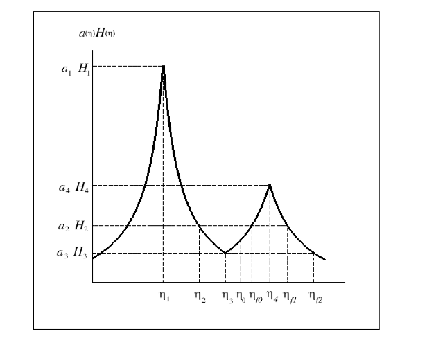
Figure 1: Evolution of $a(\eta)H(\eta)$ in a universe with scale factor given by Eq. (1). We have assumed that $a_{4}H_{4}>a_{2}H_{2}$. The quantity $\eta_{f0}$ is defined as the instant in the dark energy era in which $a(\eta_{f0})H(\eta_{f0})=a_{2}H_{2}$, $\eta_{f1}$ as the instant of the second dust era such that $a(\eta_{f1})H(\eta_{f1})=a_{2}H_{2},$ and $\eta_{f2}$ as the instant of the second dust era in which $a(\eta_{f0})H(\eta_{f0})=a_{3}H_{3}$.

The gravitational waves equation may be interpreted as the massless Klein-Gordon equation Allen ; Parker . Its solution can be written as

$$h_{ij}(\eta,\mathbf{x})=\int\left(A_{(k)}h_{ij}^{(k)}(\mathbf{k},x)+A_{(k)}^{{\dagger}}h_{ij}^{(k)}(\mathbf{k},x)\right)d^{3}k,$$ (3)

$$h_{ij}^{(k)}(\mathbf{k},x)=\frac{1}{\sqrt{\pi}}e_{ij}(\mathbf{k})\frac{\mu_{(k)}(\eta)}{a(\eta)}e^{i\mathbf{k\cdot x}}\mathbf{,}$$

$$\mu_{(k)}^{\prime\prime}(\eta)+\left(k^{2}-\frac{a^{\prime\prime}(\eta)}{a(\eta)}\right)\mu_{(k)}(\eta)=0,$$ (4)

where $A_{(k)}$, $A_{(k)}^{{\dagger}}$ are the annihilation and creation operators, respectively, $e_{ij}(\mathbf{k})$ contains the two possible polarizations of the wave and the modes $\mu_{(k)}(\eta)$ satisfy the additional condition

$$\mu_{(k)}\mu_{(k)}^{\ast\prime}-\mu_{(k)}^{\ast}\mu_{(k)}^{\prime}=i,$$ (5)

which comes from the commutation relations of the operators $A_{(k)}$, $A_{(k)}^{{\dagger}}$ and the definition of the field $h_{ij}(\eta,\mathbf{x})$ Parker ; Birrell .

To study the amplification of gravitational waves at the transition eras we must ascertain which of the solutions to (4) correspond to real particles. An approach to that problem is known as the adiabatic vacuum approximation Birrell . Basically it assumes that in the limit $k\rightarrow\infty$ the spacetime becomes asymptotically Mikowskian. In this limit the creation-destruction operators of each family of modes will correspond exactly to those associated to real particles.

Following Allen Allen and Maia Maia93 , we shall evaluate the number of RGWs created from the initial vacuum state in an expanding universe. Assuming that the scale factor in the different eras is given by Eq. (1), the initial state is the vacuum associated with the modes of the inflationary stage $\mu_{I}(\eta)$, which are a solution to the equation (4) compatible with condition (5). Taking into account the shape of the scale factor at this era the modes are

$$\mu_{I}=(\sqrt{\pi}/2)e^{i\psi_{I}}k^{-1/2}x^{1/2}H_{-3/2}^{(2)}(x),$$ (6)

where $x=k\eta$, $\psi_{I}$ an arbitrary constant phase and $H_{-3/2}^{(2)}(x)$ the Hankel function of order $-3/2$ german . Likewise, the proper modes in the radiation era are

$$\mu_{R}=(\sqrt{\pi}/2)e^{i\psi_{R}}k^{-1/2}x_{R}^{1/2}H_{1/2}^{(2)}(x_{R}),$$ (7)

where $x_{R}=k(\eta-2\eta_{1})$ and $\psi_{R}$ a constant phase.

The two families of modes are related by the Bogoliubov transformation

$$\mu_{I}(\eta)=\alpha_{1}\mu_{R}(\eta)+\beta_{1}\mu_{R}^{\ast}(\eta).$$ (8)

From the continuity of $\mu(\eta)$ at the transition time $\eta_{1}$, it follows that

$$\alpha_{1}=-1+\frac{i}{k\eta_{1}}+\frac{1}{2(k\eta_{1})^{2}},\qquad\beta_{1}=\frac{1}{2(k\eta_{1})^{2}},$$ (9)

where we have neglected an irrelevant phase. The modes with frequency $f=2\pi k/a(\eta_{1})$ at $\eta_{1}$ larger than the characteristic time scale of the transition are exponentially suppressed. This time scale is usually identified with the inverse of the Hubble factor at the transition, $H_{1}^{-1}$ in this case. Therefore, the Bogoliubov coefficients are given by $\alpha_{1}=1$ and $\beta_{1}=0$ for RGWs with $k>2\pi a_{1}H_{1}$, and by Eq. (9) when $k<2\pi a_{1}H_{1}$.

In the first dust era ($\eta_{2}<\eta<\eta_{3}$) the solution to Eq. (4) for the modes is found to be

$$\mu_{D}=(\sqrt{\pi}/2)e^{i\psi_{D}}k^{-1/2}x_{D}^{1/2}H_{3/2}^{(2)}(x_{D}),$$ (10)

where $x_{D}=k\left(\eta+\eta_{2}-4\eta_{1}\right)$ and it is related to the radiation modes by

$$\mu_{R}(\eta)=\alpha_{2}\mu_{D}(\eta)+\beta_{2}\mu_{D}^{\ast}(\eta).$$ (11)

Consequently, one obtains

$$\alpha_{2}=-i\left(1+\frac{i}{2k\eta_{R2}}-\frac{1}{8\left(k\eta_{R2}\right)^{2}}\right),\qquad\beta_{2}=\frac{i}{8\left(k\eta_{R2}\right)^{2}},$$ (12)

for $k<2\pi a(\eta_{2})H_{2}$ and $\alpha_{2}=1$, $\beta_{2}=0$ for $k>2\pi a(\eta_{2})H_{2}$, where $H_{2}$ is the Hubble factor evaluated at $\eta_{2}$ and $\eta_{R2}=\eta_{2}-2\eta_{1}$.

Finally, in the dark energy era the solution to equation (4) reads

$$\mu_{l}=(\sqrt{\pi}/2)e^{i\psi_{l}}k^{-1/2}x_{l}^{1/2}H_{l-1/2}^{(2)}(x_{l}),$$

where $x_{l}=k\eta_{l}$. The Bogoliubov transformation

$$\mu_{D}(\eta)=\alpha_{3}^{l}\mu_{l}(\eta)+\beta_{3}^{l}\mu_{l}^{\ast}(\eta)$$ (13)

relates the dust and dark energy modes.

Using the well-known relation Abr

$$H_{l-1/2}^{(2)}(x)\simeq e^{-ix}\sqrt{\frac{2}{\pi x}}\frac{(-2l)!}{(-l)!}(-2)^{l}x^{l}(1+ix),$$ (14)

valid when $x\ll 1$ and $l<-1$, it follows that

$$\alpha_{3} = \left(6(-1)^{-l}l^{l}\frac{(-2l)!}{(-l)!}\right)\eta_{m3}^{l-2}k^{l-2}+\mathcal{O}(k^{l-1}),$$

$$\beta_{3} = -\left(6(-1)^{-l}l^{l}\frac{(-2l)!}{(-l)!}\right)\eta_{m3}^{l-2}k^{l-2}+\mathcal{O}(k^{l-1}),$$

for $k<2\pi a(\eta_{3})H_{3}$ and $\alpha_{3}=1$, $\beta_{3}=0$ for $k>2\pi a(\eta_{3})H_{3}$, where $H_{3}$ is the Hubble factor evaluated at $\eta_{3}$ and $\eta_{m3}=\eta_{3}+\eta_{2}-4\eta_{1}$. The transition between the first dust era to the dark energy era has a time span of the order $H_{3}^{-1}$. This time span is much shorter than the period of the waves we are considering and therefore it may be assumed instantaneous in the calculation of the coefficients. As a consequence, the time span from this transition till today $\tau=t_{0}-t_{3}$ must be larger than $H_{3}^{-1}$, otherwise the transition first dust era-dark energy era would be too close to the present time for our formalism to apply. This condition places a bound on the value of the redshift $\frac{a_{0}}{a_{3}}$. When $l=-1$ the condition is $\frac{a_{0}}{a_{3}}>2.72$, $\frac{a_{0}}{a_{3}}>2.25$ when $l=-2$, $\frac{a_{0}}{a_{3}}>2.15$ when $l=-3$, and $\frac{a_{0}}{a_{3}}>2$ when $l\rightarrow-\infty$. This bound is compatible with the accepted values for $\frac{a_{0}}{a_{3}}\in[1.5,11]$ (see e.g., luca ). Henceforward we will consider $\frac{a_{0}}{a_{3}}$ larger than $2.72$ and no larger than $11$.

The solution to equation (4) in the second dust era (i.e., the one following the dark energy era) is

$$\mu_{SD}=(\sqrt{\pi}/2)e^{i\psi_{SD}}k^{-1/2}x_{SD}^{1/2}H_{3/2}^{(2)}(x_{SD}),$$

where $x_{SD}=k\left(\eta-\eta_{4}+\frac{2}{a_{4}H_{4}}\right)$.

The Bogoliubov coefficients relating the modes of the dark energy era with the modes of the second dust era are

$$\mu_{l}(\eta)=\alpha_{4}^{l}\mu_{SD}(\eta)+\beta_{4}^{l}\mu_{SD}^{\ast}(\eta).$$

The continuity of $\mu$ at $\eta_{4}$ implies

$$\alpha_{4}^{l} = \left(-1\right)^{l}\frac{3}{8}2^{l}\frac{(-2l)!}{(-l)!}x_{l4}^{l-2}\left[l^{2}+il(l-2)x_{l4}+\mathcal{O}(x_{l4}^{2})\right],$$

$$\beta_{4}^{l} = \left(-1\right)^{l}\frac{3}{8}2^{l}\frac{(-2l)!}{(-l)!}x_{l4}^{l-2}\left[l^{2}+il(l+2)x_{l4}+\mathcal{O}(x_{l4}^{2})\right],$$

for $k<2\pi a_{4}H_{4}$, and $\alpha_{4}^{l}=1$, $\beta_{4}^{l}=0$ for $k>2\pi a_{4}H_{4}$, where $H_{4}$ is the Hubble factor evaluated at the transition time $\eta_{4}$.

III Power spectrums

In order to relate the modes of the inflationary era to the modes of the first dust era, we make use of the total Bogoliubov coefficients $\alpha_{Tr}$ and $\beta_{Tr}$. The number of RGWs created from the initial vacuum is $\left\langle N_{\omega}\right\rangle=\left|\beta_{Tr}\right|^{2}$. Assuming that each RGW has an energy $2\hbar\omega(\eta)$ (henceforward we shall use ordinary units), the energy density of RGWs with frequencies in the range $\left[\omega(\eta),\omega(\eta)+d\omega(\eta)\right]$ can be written as

$$d\rho_{g}(\eta)=2\hbar\omega(\eta)\left[\frac{\omega^{2}(\eta)}{2\pi^{2}c^{3}}d\omega(\eta)\right]\left\langle N_{\omega}\right\rangle=P(\omega(\eta))d\omega(\eta),$$ (15)

where $P(\omega(\eta))=\left(\hbar\omega^{3}(\eta)/\pi^{2}c^{3}\right)\left\langle N_{\omega}\right\rangle$ denotes the power spectrum. As the energy density $\rho_{g}$ is a locally defined quantity, it loses its meaning for metric perturbations with wave length $\lambda=2\pi c/\omega(\eta)$ larger than the Hubble radius $cH^{-1}(\eta)$.

III.1 Current Power spectrum

To evaluate the present power spectrum one must bear in mind that $a_{0}H_{0}>a_{3}H_{3}$ which implies the perturbations created at the transition dust era-dark energy era have a wave length larger than the Hubble radius at present Chiba . One must also consider the possibility that $a_{0}H_{0}>a_{2}H_{2}$, it is to say

$$\left(\frac{a_{0}}{a_{3}}\right)^{-1/l}\left(\frac{a_{2}}{a_{3}}\right)^{1/2}>1.$$

When $l=-1$ and assuming $\frac{a_{0}}{a_{2}}\sim 10^{4}$ Peebles this condition implies $\frac{a_{0}}{a_{3}}>21.5$, $\frac{a_{0}}{a_{3}}>100$ when $l=-2,$ and $\frac{a_{0}}{a_{3}}>251.2$ when $l=-3$. The values for $\frac{a_{0}}{a_{3}}$ considered by us are larger than $2.72$ and no lower than $11$, consequently we can safely assume $a_{0}H_{0}<a_{2}H_{2}$.

For $k>2\pi a_{1}H_{1}$, we find that $\alpha_{Tr2}=1$, $\beta_{Tr2}=0$; in the range $2\pi a_{1}H_{1}>k>2\pi a_{2}H_{2}$, the coefficients are $\alpha_{Tr2}=\alpha_{1}$ and $\beta_{Tr2}=\beta_{1}$, and finally for $k<2\pi a(\eta_{2})H_{2}$ we obtain Allen ; Maia93

$$\beta_{Tr2}\simeq-\frac{1}{8k^{3}\eta_{1}^{2}\eta_{R2}}.$$ (16)

Thus, the number of RGWs at the present time $\eta_{0}$ created from the initial vacuum state is $\left\langle N_{\omega}\right\rangle=\left|\beta_{Tr2}\right|^{2}\sim\omega^{-6}(\eta_{0})$ for $\omega(\eta_{0})<2\pi(a_{2}/a_{0})H_{2}$, $\omega^{-4}(\eta_{0})$ for $2\pi(a_{1}/a_{0})H_{1}>\omega(\eta_{0})>2\pi(a_{2}/a_{0})H_{2}$, and zero for $\omega(\eta_{0})>2\pi(a_{1}/a_{0})H_{1}$, where we have used the present value of the frequency, $\omega(\eta_{0})=k/a_{0}$.

In sumary, the current power spectrum of RGWs in this scenario is

$$P(\omega)\simeq\left\{\begin{array}[]{l}0\text{\qquad}\left(\omega(\eta_{0})>2\pi(a_{1}/a_{0})H_{1}\right),\\ \\ \frac{\hbar}{4\pi^{2}c^{3}}\left(\frac{a_{1}}{a_{0}}\right)^{4}H_{1}^{4}\omega^{-1}\text{\qquad}\left(2\pi(a_{2}/a_{0})H_{2}<\omega(\eta_{0})<2\pi(a_{1}/a_{0})H_{1}\right),\\ \\ \frac{\hbar}{16\pi^{2}c^{3}}\left(\frac{a_{0}}{a_{2}}\right)^{2}\left(\frac{a_{1}}{a_{0}}\right)^{8}H_{1}^{6}\omega^{-3}\text{\qquad}\left(2\pi H_{0}<\omega(\eta_{0})<2\pi(a_{2}/a_{0})H_{2}\right).\end{array}\right.$$ (17)

While this power spectrum is not at variance with the power spectrum of the conventional three-stage scenario (De Sitter inflation, radiation and dust era) Allen ; Maia93 , it evolves differently. The power spectrum in the dark energy scenario at $\eta=\eta_{3}$ formally coincides with Eq. (17) but with $a_{3}$ substituted by $a_{0}$ throughout, and from then up to now waves with $2\pi a_{3}H_{3}<k<$ $2\pi a_{0}H_{0}$ cease to contribute to the spectrum as soon as their wave length exceeds the Hubble radius. By contrast, in the three-stage scenario waves are continuously being added to the spectrum. As we shall see in Section IV, this implies that the evolution of the energy density of the gravitational waves in the three-stage scenario differs from the scenario in which the Universe expansion is dominated by dark energy.

III.2 Power spectrum in the second dust era

In an attempt to evade the particle horizon problem posed by an everlasting accelerated expansion to string/M type theories string/M , models in which the present era is not eternal but it is followed by a decelerated phase as though dominated by cold dark matter (second dust era) were proposed Alam .

Here we evaluate the power spectrum at some future time $\eta$ larger than $\eta_{f2}$ for which the waves created at the transition dust era-dark energy era ($\eta=\eta_{3}$) are considered in the spectrum by the first time (see Figure 1). Let $\alpha_{Tr4}$ and $\beta_{Tr4}$ be the Bogoliubov coefficients relating the modes of the inflationary era to the modes of the second dust era. Because of condition (2) we must consider two possibilities with two different power spectrums.

$(i)$ If condition (2) is not fulfilled, then $a_{1}H_{1}>a_{2}H_{2}>a_{4}H_{4}>a_{3}H_{3}$ and the power spectrum can be obtained from the following total coefficients. In the range $k>2\pi a_{1}H_{1}$ the total coefficients are $\alpha_{Tr4}=1$ and $\beta_{Tr4}=0$. For $2\pi a_{1}H_{1}>k>2\pi a_{2}H_{2}$, the coefficients are $\alpha_{Tr4}=\alpha_{1}$ and $\beta_{Tr4}=\beta_{1}$, where $\alpha_{1}$ and $\beta_{1}$ are defined in Eq. (9). For $2\pi a_{2}H_{2}>k>2\pi a_{4}H_{4}$, $\alpha_{Tr4}=\alpha_{Tr2}$ and $\beta_{Tr4}=\beta_{Tr2}$ where $\alpha_{Tr2}$ and $\beta_{Tr2}$ are defined in Eq. (16).

When $2\pi a_{4}H_{4}>k>2\pi a_{3}H_{3}$, except for $\alpha_{3}$ and $\beta_{3}$, all the cofficients obtained in the previous section must be considered when evaluating $\alpha_{Tr4}$ and $\beta_{Tr4}$, therefore

$$\alpha_{Tr4}^{l} = \alpha_{4}^{l}\alpha_{Tr2}+\beta_{4}^{l\ast}\beta_{Tr2}\simeq\left[\frac{3}{32}\left(-1\right)^{-l-1}l^{2}2^{l}\frac{(-2l)!}{(-l)!}\right]\frac{2}{\eta_{1}^{2}\eta_{R2}\eta_{l4}^{-l+2}}k^{l-5},\qquad$$ (18)

$$\beta_{Tr4}^{l} = \beta_{4}^{l}\alpha_{Tr2}+\alpha_{4}^{l\ast}\beta_{Tr2}\simeq\left[\frac{3}{32}\left(-1\right)^{-l-1}l^{2}2^{l}\frac{(-2l)!}{(-l)!}\right]\frac{2}{\eta_{1}^{2}\eta_{R2}\eta_{l4}^{-l+2}}k^{l-5}.$$

Finally, for $2\pi a_{3}H_{3}>k>2\pi H(\eta)$ we get

$$\beta_{Tr4}^{l}\simeq-\left[\frac{9}{16}l^{l+2}2^{l}\left(\frac{(-2l)!}{(-l)!}\right)^{2}\right]\frac{2l}{\eta_{1}^{2}\eta_{R2}\eta_{m3}^{-l}\eta_{l4}^{-l+2}}k^{2l-5}.$$ (19)

Accordingly, the power spectrum reads

$$P(\omega)\simeq\left\{\begin{array}[]{l}0\text{\qquad}\left(\omega(\eta)>2\pi(a_{1}/a(\eta))H_{1}\right),\\ \\ \frac{\hbar}{4\pi^{2}c^{3}}\left(\frac{a_{1}}{a(\eta)}\right)^{4}H_{1}^{4}\omega^{-1}\text{\qquad}\left(2\pi(a_{2}/a(\eta))H_{2}<\omega(\eta)<2\pi(a_{1}/a(\eta))H_{1}\right),\\ \\ \frac{\hbar}{16\pi^{2}c^{3}}\left(\frac{a_{0}}{a_{2}}\right)^{2}\left(\frac{a_{1}}{a_{0}}\right)^{8}\left(\frac{a_{0}}{a(\eta)}\right)^{6}H_{1}^{6}\omega^{-3}\text{\qquad}\left(2\pi(a_{4}/a(\eta))H_{4}<\omega(\eta)<2\pi(a_{2}/a(\eta))H_{2}\right)\\ \\ \frac{9\hbar}{\pi^{2}c^{3}}l^{2l}2^{2l-8}\left(\frac{(-2l)!}{(-l)!}\right)^{2}\left(\frac{a_{1}}{a_{0}}\right)^{16-4l}\left(\frac{a_{2}}{a_{0}}\right)^{l-4}\left(\frac{a_{3}}{a_{0}}\right)^{l-4+4/l}\left(\frac{a_{4}}{a_{0}}\right)^{-8+2l-4/l}\\ \text{\qquad}\times\left(\frac{a(\eta)}{a_{4}}\right)^{2l-10}H_{1}^{10-2l}\omega^{2l-7}\text{\qquad}\left(2\pi(a_{3}/a(\eta))H_{3}<\omega(\eta)<2\pi(a_{4}/a(\eta))H_{4}\right),\\ \\ \frac{27\hbar}{\pi^{2}c^{3}}l^{4l}2^{4l-6}\left(\frac{(-2l)!}{(-l)!}\right)^{4}\left(\frac{a_{1}}{a_{0}}\right)^{16-8l}\left(\frac{a_{2}}{a_{0}}\right)^{2l-4}\left(\frac{a_{3}}{a_{0}}\right)^{2l-4+4/l}\left(\frac{a_{4}}{a_{0}}\right)^{4l-8-4/l}\\ \text{\qquad}\times\left(\frac{a(\eta)}{a_{4}}\right)^{4l-10}H_{1}^{10-4l}\omega^{4l-7}\text{\qquad}\left(2\pi H(\eta)<\omega(\eta)<2\pi(a_{3}/a(\eta))H_{3}\right).\end{array}\right.$$

$(ii)$ If condition (2) is fulfilled, then $a_{1}H_{1}>a_{4}H_{4}>a_{2}H_{2}>a_{3}H_{3}$. As in the previous case, in the range $k>2\pi a_{1}H_{1}$ the total coefficients are $\alpha_{Tr4}=1$ and $\beta_{Tr4}=0$. For $2\pi a_{1}H_{1}>k>2\pi a_{4}H_{4}$, the coefficients are $\alpha_{Tr4}=\alpha_{1}$ and $\beta_{Tr4}=\beta_{1}$. In the range $2\pi a_{4}H_{4}>k>2\pi a_{2}H_{2}$, we obtain

$$\alpha_{Tr4}^{l} = \alpha_{4}^{l}\alpha_{1}+\beta_{4}^{l\ast}\beta_{1}\simeq i\frac{3}{8}\left(-1\right)^{-l}l^{2}2^{l}\frac{(-2l)!}{(-l)!}\frac{1}{\eta_{1}^{2}\eta_{l4}^{-l+1}}k^{l-3},\qquad$$

$$\beta_{Tr4}^{l} = \beta_{4}^{l}\alpha_{1}+\alpha_{4}^{l\ast}\beta_{1}\simeq i\frac{3}{8}\left(-1\right)^{-l}l^{2}2^{l}\frac{(-2l)!}{(-l)!}\frac{1}{\eta_{1}^{2}\eta_{l4}^{-l+1}}k^{l-3}.$$

Again, for $2\pi a_{2}H_{2}>k>2\pi a_{3}H_{3}$, the total coefficients are given by Eq. (18) while for $2\pi a_{3}H_{3}>k>2\pi H(\eta)$ they obey Eq. (19). The power spectrum in this case is

$$P(\omega)\simeq\left\{\begin{array}[]{l}0\text{\qquad}\left(\omega(\eta)>2\pi(a_{1}/a(\eta))H_{1}\right),\\ \\ \frac{\hbar}{4\pi^{2}c^{3}}\left(\frac{a_{1}}{a(\eta)}\right)^{4}H_{1}^{4}\omega^{-1}\text{\qquad}\left(2\pi(a_{4}/a(\eta))H_{4}<\omega(\eta)<2\pi(a_{1}/a(\eta))H_{1}\right),\\ \\ \frac{9\hbar}{\pi^{2}c^{3}}l^{2l+2}2^{2l-6}\left(\frac{(-2l)!}{(-l)!}\right)^{2}\left(\frac{a_{1}}{a_{0}}\right)^{8-4l}\left(\frac{a_{2}}{a_{0}}\right)^{l-1}\left(\frac{a_{3}}{a_{0}}\right)^{l-3+2/l}\left(\frac{a_{4}}{a_{0}}\right)^{2l-4-4/l}\\ \text{\qquad}\times\left(\frac{a(\eta)}{a_{4}}\right)^{2l-6}H_{1}^{6-2l}\omega^{2l-3}\text{\qquad}\left(2\pi(a_{2}/a(\eta))H_{2}<\omega(\eta)<2\pi(a_{4}/a(\eta))H_{4}\right),\\ \\ \frac{9\hbar}{\pi^{2}c^{3}}l^{2l}2^{2l-8}\left(\frac{(-2l)!}{(-l)!}\right)^{2}\left(\frac{a_{1}}{a_{0}}\right)^{16-4l}\left(\frac{a_{2}}{a_{0}}\right)^{l-4}\left(\frac{a_{3}}{a_{0}}\right)^{l-4+4/l}\left(\frac{a_{4}}{a_{0}}\right)^{2l-8-4/l}\\ \text{\qquad}\times\left(\frac{a(\eta)}{a_{4}}\right)^{2l-10}H_{1}^{10-2l}\omega^{2l-7}\text{\qquad}\left(2\pi(a_{3}/a(\eta))H_{3}<\omega(\eta)<2\pi(a_{2}/a(\eta))H_{2}\right),\\ \\ \frac{27\hbar}{\pi^{2}c^{3}}l^{4l}2^{4l-6}\left(\frac{(-2l)!}{(-l)!}\right)^{4}\left(\frac{a_{1}}{a_{0}}\right)^{16-8l}\left(\frac{a_{2}}{a_{0}}\right)^{2l-4}\left(\frac{a_{3}}{a_{0}}\right)^{2l-4+4/l}\left(\frac{a_{4}}{a_{0}}\right)^{4l-8-4/l}\\ \text{\qquad}\times\left(\frac{a(\eta)}{a_{4}}\right)^{4l-10}H_{1}^{10-4l}\omega^{4l-7}\text{\qquad}\left(2\pi H(\eta)<\omega(\eta)<2\pi(a_{3}/a(\eta))H_{3}\right).\end{array}\right.$$ (20)

The power spectrum governed by Eq.(20) is plotted in Fig. 2 for different choices of the free parameters $l$, $\frac{a_{0}}{a_{3}}$, $\frac{a_{4}}{a_{0}}$ and $\frac{a(\eta)}{a_{0}}$ as well as the power spectrum assuming the three-stage model, i.e., non-accelerated phase and no second dust era.

The shape of the power spectrum given by (20) in the range $2\pi H(\eta)<\omega(\eta)<2\pi(a_{3}/a(\eta))H_{3}$ is the same in both cases as in this range all the coefficients are present in the evaluation of the total coefficients. It is interesting to see how markedly this spectrum differs from the one arising in the three-stage model (dot-dashed line) at low wave lengths.

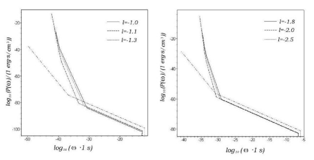
Figure 2: Power spectrum given by Eq. (20) for different values of $l$. The left panel depicts the power spectrum at the instant $\eta$ for which $\frac{a\left(\eta\right)}{a_{0}}=10^{22}$ (when $\Omega_{g}(\eta)$ is near unity), with $\frac{a_{0}}{a_{3}}=11$, and $\frac{a_{4}}{a_{0}}=10^{6}$ (to fulfill condition (2)). The right panel shows the power spectrum at the instant $\eta$ for which $\frac{a\left(\eta\right)}{a_{0}}=10^{16}$ (again when $\Omega_{g}(\eta)$ is near unity), with $\frac{a_{0}}{a_{3}}=11$, and $\frac{a_{4}}{a_{0}}=10^{6}$. For the sake of comparison the power spectrum of the three-stage scenario (De Sitter inflation, radiation, dust with $l=2$) is also shown in both panels (dot-dashed line). Notice the difference in slopes at the dust era.

III.2.1 Topological defects

Up to now we assumed that at the end of the dark energy era the Universe will evolve as if it became dominated by dust once again. Nevertheless if the expansion achieved in the accelerated phase were large enough, either cosmic strings, or domain walls, or a cosmological constant will take over instead. We will not consider, however, cosmic strings (whose equation of state is $p_{K}=-\frac{1}{3}\rho_{K}$) for, as pointed out by Maia Maia93 , it seems problematic to define an adiabatic vacuum in an era dominated by these topological defects since the creation–anihilation operators, $A_{(k)}$, $A_{(k)}^{{\dagger}}$, fail to satisfy the conmutation relations (i. e., condition (5)) in the range of frequencies where one should expect RGWs amplification. In short, our approach, as it is, does not apply to this case.

As for domain walls (topological stable defects of second order with equation of state $p_{dw}=-\frac{2}{3}\rho_{dw}$ and energy density that varies as $a^{-1}(\eta)$ -see e.g., Kolb ; shellard ), once the dark energy evolved as pressureless matter at $\eta=\eta_{4}$ the scale factor may be approximated by

$$a(\eta>\eta_{4})=4a_{4}\left(a_{4}H_{4}\right)^{-2}\left(-\eta+\eta_{4}+\frac{2}{a_{4}H_{4}}\right)^{-2},$$

so long as $a^{-1}\gg$ $a^{-3}$. That is to say, for $\eta>\eta_{4}$ the expansion of the Universe is again accelerated whereby $a(\eta)H(\eta)$ resumes growing. The RGWs will be leaving the Hubble radius as soon as $cH^{-1}$ becomes smaller than their wave length, and eventually none of them will contribute to the spectrum.

Finally, we consider the existence of a positive cosmological constant $\Lambda$ with $\rho_{\Lambda}=\Lambda/\left(8\pi\right)$ and $p_{\Lambda}=-\rho_{\Lambda}$. After the dark energy dynamically mimicked dust the Universe will become dominated by a very tiny cosmological constant. The corresponding scale factor is

$$a(\eta>\eta_{4})=H_{4}^{-1}\left(-\eta+\eta_{4}+\frac{1}{a_{4}H_{4}}\right)^{-1}.$$

Once more, the expansion is accelerated and RGWs will leave the Hubble radius and eventually none of them will contribute to the spectrum.

IV Energy density of the gravitational waves

By integrating the power spectrum $P(\omega)$, defined by Eq. (15), one can obtain the energy density of the RGWs in terms of the conformal time. Its current value, evaluated from Eq. (17), can be aproximated by Allen

$$\rho_{g}(\eta_{0})\simeq\frac{\hbar}{32\pi^{2}c^{3}}\left(\frac{a_{0}}{a_{2}}\right)^{2}\left(\frac{a_{1}}{a_{0}}\right)^{8}H_{1}^{6}(2\pi H_{0})^{-2}.$$ (21)

To study the evolution of $\rho_{g}(\eta)$ from this point onward we first consider the case $a_{4}H_{4}>a_{2}H_{2}$. In this case, $\rho_{g}(\eta)$ evolves as (21) with $H(\eta)$ and $a(\eta)$ substituted by $H_{0}$ and $a_{0}$, respectively, till some instant $\eta_{f0}$ in the range $\eta_{0}<\eta_{f0}<\eta_{4}$. When $\eta\geqslant\eta_{f0}$ the RGWs with $\omega(\eta_{f0})<2\pi\left(a_{2}/a(\eta_{f0})\right)H_{2}$ must no longer be considered in evaluating $\rho_{g}$ as their wave length exceed the Hubble radius. Consequently

$$\rho_{g}(\eta_{f0}<\eta<\eta_{4})\simeq\frac{\hbar}{4\pi^{2}c^{3}}\left(\frac{a_{1}}{a(\eta)}\right)^{4}H_{1}^{4}\ln\left(\frac{a_{1}H_{1}}{a(\eta)H(\eta)}\right).$$ (22)

For $\eta=\eta_{4}$, the gravitational waves created at the transition dark energy era-second dust era begin contriubuting to $\rho_{g}$ thereby,

$$\rho_{g}(\eta_{4} < \eta<\eta_{f1})\simeq\rho_{g}(\eta_{4})\left(\frac{a_{4}}{a\left(\eta\right)}\right)^{4}+\frac{9\hbar}{\pi^{2}c^{3}}l^{2l+2}2^{2l-6}\left(\frac{(-2l)!}{(-l)!}\right)^{2}\left(\frac{a_{1}}{a_{0}}\right)^{8-4l}$$

$$\times\left(\frac{a_{2}}{a_{0}}\right)^{l-1}\left(\frac{a_{3}}{a_{0}}\right)^{l-3+2/l}\left(\frac{a_{4}}{a_{0}}\right)^{2l-4-4/l}\left(\frac{a(\eta)}{a_{4}}\right)^{2l-6}H_{1}^{6-2l}\frac{(2\pi H(\eta))^{2l-2}}{-2l+2},$$

where $\rho_{g}(\eta_{4})$ corresponds to Eq.(22) evaluated at $\eta=\eta_{4}$. For $\eta=\eta_{f1}>\eta_{4}$ where $\eta_{f1}$ is defined by the condition $a(\eta_{f1})H(\eta_{f1})=a_{2}H_{2}$ (see Figure 1), the garvitational waves which left the Hubble radius at $\eta_{f0}$ reenter it, therefore

$$\rho_{g}(\eta_{f1} < \eta<\eta_{f2})\simeq\rho_{g}(\eta_{f1})\left(\frac{a_{f1}}{a\left(\eta\right)}\right)^{4}+\frac{9\hbar}{\pi^{2}c^{3}}l^{2l}2^{2l-8}\left(\frac{(-2l)!}{(-l)!}\right)^{2}\left(\frac{a_{1}}{a_{0}}\right)^{16-4l}$$

$$\times\left(\frac{a_{2}}{a_{0}}\right)^{l-4}\left(\frac{a_{3}}{a_{0}}\right)^{l-4+4/l}\left(\frac{a_{4}}{a_{0}}\right)^{2l-8-4/l}\left(\frac{a(\eta)}{a_{4}}\right)^{2l-10}H_{1}^{10-2l}\frac{(2\pi H(\eta))^{2l-6}}{-2l+6},$$

where $\rho_{g}(\eta_{f1})$ corresponds to Eq.(IV) evaluated at $\eta=\eta_{f1}$. For $\eta=\eta_{f2}$, with $\eta_{f2}$ defined by $a(\eta_{f2})H(\eta_{f2})=a_{3}H_{3}$ (see Figure 1), the gravitational waves created at the transition first dust era-dark energy era have wave lengths shorter than the Hubble radius for first time, and from that point on the density of gravitational waves can be aproximated by

$$\rho_{g}(\eta > \eta_{f2})\simeq\rho_{g}(\eta_{f2})\left(\frac{a_{f2}}{a\left(\eta\right)}\right)^{4}+\frac{27\hbar}{\pi^{2}c^{3}}l^{4l}2^{4l-6}\left(\frac{(-2l)!}{(-l)!}\right)^{4}\left(\frac{a_{1}}{a_{0}}\right)^{16-8l}$$

$$\times\left(\frac{a_{2}}{a_{0}}\right)^{2l-4}\left(\frac{a_{3}}{a_{0}}\right)^{2l-4+4/l}\left(\frac{a_{4}}{a_{0}}\right)^{4l-8-4/l}\left(\frac{a(\eta)}{a_{4}}\right)^{4l-10}H_{1}^{10-4l}\frac{(2\pi H(\eta))^{4l-6}}{-4l+6},$$

where $\rho_{g}(\eta_{f2})$ corresponds to Eq.(IV) evaluated at $\eta=\eta_{f2}$.

In the case that $a_{4}H_{4}>a_{2}H_{2}$, Eq. (21) dictates the evolution of $\rho_{g}$ between $\eta_{0}$ till $\eta_{4}$. Then, from $\eta_{4}$ till $\eta_{f2}$, $\rho_{g}$ obeys Eq. (IV) (note that $\eta_{f1}$ cannot be defined in this case) and from $\eta_{f2}$ onwards $\rho_{g}$ obeys Eq. (IV).

A natural restriction on $\rho_{g}(\eta)$ is that it must be lower than the total energy density of the flat FRW Universe

$$\rho(\eta)=\frac{c}{\hbar}\frac{3m_{Pl}^{2}}{8\pi}H^{2}(\eta),$$

where $m_{Pl}$ stands for the Planck mass.

It seems reasonable to consider $H_{1}\simeq 10^{38}s^{-1}$ as it corresponds to the GUT model of inflation bruce ; alan . The redshift $\frac{a_{0}}{a_{2}}$, relating the present value of the scale factor with the scale factor at the transition radiation era-first dust era, may be taken as $10^{4}$ Peebles , and the current value of the Hubble factor $H_{0}$ is estimated to be $2.24\times 10^{-18}s^{-1}$ Spergel . It then follows

$$\frac{a_{1}}{a_{0}} = 1.50\times 10^{-29}\left(\frac{a_{0}}{a_{3}}\right)^{-\frac{1}{4}+\frac{1}{2l}},\text{\qquad}H_{2}=2.24\times 10^{-12}\left(\frac{a_{0}}{a_{3}}\right)^{-\frac{1}{2}+\frac{1}{l}}s^{-1},$$

$$H_{3} = H_{0}\left(\frac{a_{0}}{a_{3}}\right)^{1+\frac{1}{l}}s^{-1},\text{\qquad}H_{4}=H_{0}\left(\frac{a_{4}}{a_{0}}\right)^{-1-\frac{1}{l}}s^{-1},$$

$$H_{f1} = 2.24\times 10^{-12}\left(\frac{a_{0}}{a_{3}}\right)^{-\frac{3}{2}+\frac{3}{l}}\left(\frac{a_{4}}{a_{0}}\right)^{-1+\frac{2}{l}}s^{-1},$$

$$H_{f2} = 2.24\times 10^{-18}\left(\frac{a_{0}}{a_{3}}\right)^{\frac{3}{l}}\left(\frac{a_{4}}{a_{0}}\right)^{-1+\frac{2}{l}}s^{-1},$$

where we have used the relation

$$H(\eta>\eta_{4})=\left(\frac{a_{4}}{a(\eta)}\right)^{3/2}H_{4},$$ (26)

valid in the second dust era (see Eq. (1)) with $a_{f1}H_{f1}=a_{2}H_{2}$ and $a_{f2}H_{f2}=a_{3}H_{3}$ to evaluate $H_{f1}$ (only defined if $a_{4}H_{4}>a_{2}H_{2}$) and $H_{f2}$, respectively. In our model, there are only three parameters, namely $l\leq-1$, $2.72<\frac{a_{0}}{a_{3}}<11$, and $\frac{a_{4}}{a_{0}}$.

We are now in position to evaluate the evolution of the dimensionless density parameter $\Omega_{g}(\eta)\equiv\rho_{g}(\eta)/\rho(\eta)$. Its current value is Allen

$$\Omega_{g0}\simeq\frac{1}{48\pi^{3}}\frac{G\hbar}{c^{5}}\left(\frac{a_{0}}{a_{2}}\right)^{2}\left(\frac{a_{1}}{a_{0}}\right)^{8}H_{1}^{6}H_{0}^{-4},$$

which in our description boils down to

$$\Omega_{g0}\simeq 2.00\times 10^{-13}\left(\frac{a_{0}}{a_{3}}\right)^{-2+\frac{4}{l}}.$$ (27)

$\Omega_{g0}$ is much lower than unity for any choice of $\frac{a_{0}}{a_{3}}$ and $l$ in the above intervals. At later times $\Omega_{g}$ evolves as

$$\Omega_{g}(\eta>\eta_{0})=\Omega_{g0}\left(\frac{a(\eta)}{a_{0}}\right)^{-2+\frac{4}{l}},$$ (28)

where we have used $H(\eta_{4}>\eta>\eta_{0})=\left(\frac{a(\eta)}{a_{0}}\right)^{-1-\frac{1}{l}}H_{0}$. It is obvious that $\Omega_{g}(\eta)$ is a decreasing function of $\eta$. For $\eta>\eta_{0}$ we shall distinguish the two cases mentioned in the previous section.

When condition (2) is fulfilled, the evolution of $\Omega_{g}$ is given by Eq. (28) till $\eta=\eta_{f0}$. Then, $\rho_{g}$ changes in shape from $\eta=\eta_{f0}$ till $\eta=\eta_{4}$, as we have seen. Consequently,

$$\Omega_{g}(\eta_{4} > \eta>\eta_{f0})\simeq\frac{2}{3\pi}\frac{G\hbar}{c^{5}}\left(\frac{a_{0}}{a_{3}}\right)^{-1+\frac{2}{l}}\frac{a_{2}}{a_{0}}\left(\frac{a(\eta)}{a_{0}}\right)^{-2+\frac{2}{l}}H_{1}^{2}$$

$$\times\ln\left[\left(\frac{a_{2}}{a_{0}}\right)^{\frac{1}{4}}\left(\frac{a_{0}}{a_{3}}\right)^{\frac{1}{4}-\frac{1}{2l}}\left(\frac{a(\eta)}{a_{0}}\right)^{\frac{1}{l}}H_{1}^{\frac{3}{2}}H_{0}^{-\frac{1}{2}}\right],$$

is a decreasing function of $\eta$. Finally, from $\eta_{4}$ on, $\Omega_{g}$ evolves as

$$\Omega_{g}(\eta_{f1} > \eta>\eta_{4})\simeq\Omega_{g}(\eta_{4})\left(\frac{a_{4}}{a(\eta)}\right)+\frac{24}{\pi}\frac{G\hbar}{c^{5}}l^{2l+2}2^{2l-6}\left(\frac{(-2l)!}{(-l)!}\right)^{2}\left(\frac{a_{1}}{a_{0}}\right)^{8-4l}$$

$$\times\left(\frac{a_{2}}{a_{0}}\right)^{l-1}\left(\frac{a_{3}}{a_{0}}\right)^{l-3+2/l}\left(\frac{a_{4}}{a_{0}}\right)^{2l-4-4/l}\left(\frac{a(\eta)}{a_{4}}\right)^{2l-6}H_{1}^{6-2l}\frac{(2\pi)^{2l-2}}{-2l+2}\left(H(\eta)\right)^{2l-4},$$

$$\Omega_{g}(\eta_{f2} > \eta>\eta_{f1})\simeq\Omega_{g}(\eta_{f1})\left(\frac{a_{f1}}{a(\eta)}\right)+\frac{24}{\pi}\frac{G\hbar}{c^{5}}l^{2l}2^{2l-8}\left(\frac{(-2l)!}{(-l)!}\right)^{2}\left(\frac{a_{1}}{a_{0}}\right)^{16-4l}$$

$$\times\left(\frac{a_{2}}{a_{0}}\right)^{l-4}\left(\frac{a_{3}}{a_{0}}\right)^{l-4+4/l}\left(\frac{a_{4}}{a_{0}}\right)^{2l-8-4/l}\left(\frac{a(\eta)}{a_{4}}\right)^{2l-10}H_{1}^{10-2l}\frac{(2\pi)^{2l-6}}{-2l+6}\left(H(\eta)\right)^{2l-8},$$

$$\Omega_{g}(\eta > \eta_{f2})\simeq\Omega_{g}(\eta_{f2})\left(\frac{a_{f2}}{a(\eta)}\right)+\frac{72}{\pi}\frac{G\hbar}{c^{5}}l^{4l}2^{4l-6}\left(\frac{(-2l)!}{(-l)!}\right)^{4}\left(\frac{a_{1}}{a_{0}}\right)^{16-8l}$$

$$\times\left(\frac{a_{2}}{a_{0}}\right)^{2l-4}\left(\frac{a_{3}}{a_{0}}\right)^{2l-4+4/l}\left(\frac{a_{4}}{a_{0}}\right)^{4l-8-4/l}\left(\frac{a(\eta)}{a_{4}}\right)^{4l-10}H_{1}^{10-4l}\frac{(2\pi)^{4l-6}}{-4l+6}\left(H(\eta)\right)^{4l-8}.$$

As follows from (26) and (IV)-(IV), in each case, the first term redshifts with expansion while the second term of $\Omega_{g}$ grows with $\eta$ (recall that $l\leq-1$). Conditions $\Omega_{g}(\eta_{f1}>\eta>\eta_{4})\ll 1$ and $\Omega_{g}(\eta_{f2}>\eta>\eta_{f1})\ll 1$ become just $\Omega_{g}(\eta=\eta_{f1})\ll 1$ and $\Omega_{g}(\eta=\eta_{f2})\ll 1$, which are true in either case whatever the choice of parameters. Finally, from Eq. (IV) we may conclude that at some future time larger than $\eta_{f2}$ the condition $\Omega_{g}\ll 1$ will no longer be fulfilled and the linear aproximation in which our approach rests will cease to apply.

In the opposite case, when condition (2) is not fulfilled, $\Omega_{g}$ also grows following Eq. (28) till $\eta=\eta_{4}$, in the interval $\eta_{4}<\eta<\eta_{f2}$ it grows according to Eq. (IV), and according to Eq. (IV) from $\eta_{f2}$ onwards. Our conclusions of the first case regarding the evolution of $\Omega_{g}$ during these time intervals still hold true.

The behavior of the density parameter $\Omega_{g}$ differs from one scenario to the other. In the three stage model (inflation, radiation, dust) $\Omega_{g}$ remains constant during the dust era Allen . In a four stage model, with a dark energy era right after the conventional dust era, $\Omega_{g}$ sharply decreases in a $l$ dependent way during the fourth (accelerated) era since long wavelenghts are continuously exiting the Hubble sphere Chiba , see Fig. 3.

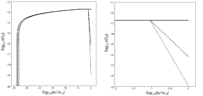
Figure 3: Left panel: Evolution of the density parameter $\Omega_{g}$ with the scale factor from the beginning of the radiation era till the present time. The solid line shows the density parameter predicted by the three-stage model (De Sitter inflation, radiation, dust). The dashed and dotted lines depict the density parameter predicted by a four-stage model having a dark energy era right after the dust era with $l=-3,\,-1$, respectively, and $a_{0}/a_{3}=11$. Note that the four-stage model predicts a lower present value for $\Omega_{g}$ than the three-stage one as $\Omega_{g}$ decreases, in a $l$ dependent fashion, during the dark energy era. The right panel is a blow up of the region in which the four stage models ($l=-3,\,-1$), notably differ from the three stage one.

By contrast, if a second dust era followed the accelerated (dark energy) era, $\Omega_{g}$ would grow in this second dust era because long wavelenghts would continuously be entering that sphere, see Fig. 4. This immediately suggests a criterion to be used by future observers to ascertain whether the era they are living in is still our accelerated, dark energy-dominated, era or a subsequent non-accelerated era. By measuring $\Omega_{g}$ at conveniently spaced instants they shall be able to tell. Further, if that era were the accelerated one and the $\Omega_{g}$ measurements were accurate enough they will be able to find out the value of the parameter $l$ occurring in the expansion law given by Eq. (1). The lower $l$, the higher the slope of $\Omega_{g}$ in the second dust era.

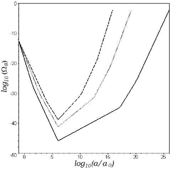
Figure 4: Evolution of the density parameter $\Omega_{g}$ given by Eqs. (27)-(IV) with the scale factor in a five-stage scenario (De Sitter inflation-radiation-dust-dark energy-second dust era) from the beginning of the dark energy era. The second dust era starts at the time in which the graphs attain their minimum. The solid, dotted and dashed lines correspond to $l=-1$, $l=-1.5$ and $l=-2$, respectively. The density parameter decreases in the dark energy era and increases in the second dust era till its value is comparable to unity. From that point on our approach (being linear) ceases to apply. We have chosen a dark energy era which begins when $a_{3}/a_{0}=1/11$ and ends when $a_{4}/a_{0}=10^{6}$.

One may argue, however, that these observers may know more easily from supernova data. Nonetheless, if this epoch lays in the far away future it may well happen that by then the ability of galaxies to generate stars (and hence enough supernovae) has seriously gone down and as a result this prime method might be unavalaible or severely impared. At any rate, even if there were plenty of supernova, the simple gravitational wave method just outlined could still play a complementary role.

V Discussion

We have studied the power spectrum and the energy density evolution of the relic gravitational waves generated at the big bang by considering the transitions between sucessive stages of the Universe expansion. In particular, we have studied the effect of the present phase of accelerated expansion as well as a hypothetical second dust phase that may come right after the present one. As it turns out, the power spectrum at the current accelerated era Eq.(17) formally coincides with the power spectrum of the usual three-stage scenario. As a consequence, measurements of $P(\omega)$ will not directly tell us if the Universe expansion is currently accelerated (as we know from the high redshift supernove data) or non-accelerated. However, the density parameter of the gravitational waves evolves differently during these two phases: it stays constant in the decelerated one and goes down in the accelerated era in a $l$ dependent manner. Therefore, the present value of $\Omega_{g}$ may not only confirm us the current acceleration but also may help determine the value the parameter $l$ -see Fig. 3- and hence give us invaluable information about the nature of dark energy.

In the far away future measurements of $P(\omega)$, if sufficciently accurate, will be able to tell if the Universe is still under accelerated expansion (driven by dark energy) or has entered a hypothetical decelerated phase (second dust era) suggested by different authors Alam . This may also be ascertained by measuring the density parameter of the gravitational waves at different instants to see whether it decreases or increases.

References

• (1) K.S. Thorne, in 300 Hundred Years of Gravitation, edited by S.W. Hawking and W. Israel (Cambridge University Press, Cambridge, 1987).
• (2) A. Buonanno, Lecture given at the Theoretical Advanced Study Institute in Elementary Particle Physics at the University of Colorado at Boulder, preprint gr-qc/0303085.
• (3) B. Allen, “The stochastic gravity-wave background: sources and detection”, in Proceedings of the Les Houches School on Astrophysical Sources of Gravitational Waves, edited by J.A. Marck et al. (Cambridge University Press, Cambridge, 1996), preprint gr-qc/9604033.
• (4) L.P. Grishchuk, Sov. Phys. JETP 40, 409 (1975); Ann. N.Y. Acad. Sci. 302, 439 (1977); Class. Quantum Grav. 10, 2449 (1993).
• (5) B. Allen, Phys. Rev. D 37, 2078 (1987).
• (6) M. R. de Garcia Maia, Phys. Rev. D 48, 647 (1993).
• (7) G. Izquierdo and D. Pavón, Phys. Rev. D 8, 12400 5 (2003).
• (8) Ch. Misner, Nature 214, 40 (1967); L.P. Grischuk and A.G. Polnarev in General Relativity and Gravitation vol. 2, edited by A. Held (Plenum, New York, 1980); V. Méndez, D. Pavón and J.M. Salim, Class. Quantum Grav. 14, 77 (1997).
• (9) http://lisa.jpl.nasa.gov
• (10) A. Riess et al., Astron. J. 116, 1009 (1998); P. Garnavich et al., Astrophys. J. 509, 74 (1998); S. Perlmutter et al., Astrophys. J. 517, 565 (1999); D.N. Spergel et al., Astrophys. J. Suppl. 148, 175 (2003); R.A. Knop et al., preprint astro-ph/0309368.
• (11) Proceedings of the I.A.P. Conference “On the Nature of Dark Energy”, Paris 2002, edited by P. Brax, J. Martin and J.P. Uzan (Frontier Group, Paris 2002);
S. Carroll, preprint astro-ph/0310342; V. Sahni, Class. Quantum Grav. 19, 3435 (2002); V. Sahni, in Proceedings of the Second Aegean Summer School on the Early Universe, Syros, Greece, 2003, preprint astro-ph/0403324.
• (12) U. Alam, V. Sahni, A. A. Starobinsky, JCAP 0304, 02 (2003); M. Sami, T. Padmanabhan, Phys. Rev. D 67, 083509 (2003); R. Kallosh and A. Linde, Phys. Rev. D 67, 023510 (2003); V. Sahni and Yu. V, Shtanov, JCAP 0311, 014 (2003).
• (13) L. H. Ford, L. Parker, Phys. Rev. D 16, 1601 (1977).
• (14) N. D. Birrell, P. C. W. Davies, Quantum Fields in Curved Space (Cambridge University Press, 1982).
• (15) M. Abramowitz and I.A. Stegun, eds., Handbook of Mathematical Functions(Dover, New York, 1972).
• (16) L. Amendola, Mon. Not. Roy. Astron. Soc. 342, 221 (2003), preprint astro-ph/0209494; L.P. Chimento, A.S. Jakubi, D. Pavón and W. Zimdahl, Phys. Rev. D 67, 083513 (2003).
• (17) H. Tashiro, T. Chiba and M. Sasaki, Class. Quantum Grav. 21, 1761 (2004).
• (18) P. J. E. Peebles, Principles of Physical Cosmology (Princeton University Press, Princeton, 1993).
• (19) J.M. Cline, J. High Energy Physics 8, 35 (2001).
• (20) E. W. Kolb, M. S. Turner, The Early Universe (Addison-Wesley, Redwood City, 1990).
• (21) A. Vilenkin and E. Shellard, Cosmic Strings and other Topological Defects (Cambridge University Press, Cambridge, 1994).
• (22) A.H. Guth, Phys. Rev. D 23, 347 (1981).
• (23) D. N. Spergel et al., Astrophys. J. Suppl. 148, 175 (2003).