Abundance Stratification in Type Ia Supernovae:
i. The Case of SN 2002bo

Abstract

The abundance stratification in the ejecta of the normal Type Ia Supernova 2002bo is derived fitting a series of spectra obtained at close time intervals. A Montecarlo code, modified to include abundance stratification, is used to compute synthetic spectra at 13 epochs in the photospheric phase, starting 13 days before $B$ maximum. A description of the abundance distribution above 7600 km s^-1 is thus obtained. Abundances in deeper layers, down to zero velocity, are derived from models of two nebular-phase spectra. Elements synthesised in different stages of burning are significantly, but not completely mixed in the ejecta. A total ⁵⁶Ni mass of 0.52 M_⊙ is derived. Evidence for intermediate-mass elements at high velocities ($\ga 18,000$ km s^-1) is found, most clearly in Si ii 6355 Å, Ca ii H&K, and in the Ca ii IR triplet. Carbon lines are not seen at any velocity, with possible implications on the progenitor/explosion scenario. A synthetic bolometric light curve computed using the inferred abundance distribution is in very good agreement with the observed one, providing an independent check. In particular, the fast rise of the light curve is reproduced very well. This is due to outward mixing of ⁵⁶Ni, which is clearly well determined by the spectroscopic modelling.

1 Introduction

It is widely agreed that Type Ia Supernovae (SNe Ia) result from the thermonuclear explosion of Carbon-Oxygen white dwarfs (WD) in binary systems. Two possible progenitor configurations are usually considered. In the single degenerate scenario a WD accretes mass from a Roche lobe-filling Red Giant companion. When the WD reaches a mass close to the Chandrasekhar limit ($\approx$ 1.38 M_⊙), carbon burning is triggered by compressional heating near the centre. After a few thousand years of quiet burning (Iben & Tutukov, 1984; Webbink, 1984; Woosley, Wunsch & Kuhlen, 2004), a thermonuclear runaway occurs which disrupts the star. In the double degenerate scenario, two low-mass WDs in a close binary system with total mass exceeding the Chandrasekhar mass lose angular momentum via the emission of gravitational waves, which ultimately leads to the merging of the two stars and to a thermonuclear runaway (Whelan & Iben, 1973; Nomoto, 1982; Han & Podsiadlowski, 2004). Potential progenitor systems for both channels have been detected, but their numbers are too low to explain the frequency of occurrence of SNe Ia (Cappellaro, Evans & Turatto, 1999).

Although the apparent predictability and homogeneity of SNe Ia, together with their brightness, has motivated their use as standardisable cosmological candles (Perlmutter et al., 1999; Riess et al., 1998), much remains unknown about their properties, as regards both global physical processes and the peculiarities of individual objects.

For example, the details of the explosion process are still unclear. Ignition is supposed to start near the centre. A subsonic (deflagration) wave, often called a “flame”, travels outwards, burning part of the WD to nuclear statistical equilibrium (NSE). The subsonic speed of the deflagration front prevents the WD from being burned to NSE entirely. Partial burning of C and O results in the production of intermediate mass elements (IME): Si, S, Mg and Ca dominate the early spectra of SNe Ia. The prompt detonation mechanism (Arnett, 1969), on the other hand, is inconsistent with the spectra, as it fails to produce sufficient amounts of IME. There is still no agreement as to whether the explosion continues as a deflagration, becoming strongly turbulent (Nomoto, Thielemann & Yokoi 1984; Woosley, Axelrod & Weaver, 1984; Niemeyer & Hillebrandt, 1995; Reinecke, Hillebrandt & Niemeyer, 2002) or it turns to a supersonic detonation. Recent 3D deflagration models leave significant amounts of unburned material both in the outer and in the inner parts of the ejecta (Gamezo et al., 2003; Reinecke et al., 1999; Travaglio et al., 2004), and produce too little radioactive ⁵⁶Ni. This could affect the light curve of SNe Ia, which is powered by ⁵⁶Ni through the energy released in the decay chain to stable ⁵⁶Fe via ⁵⁶Co. Presently, delayed detonation models (Höflich & Khokhlov, 1996; Iwamoto et al., 1999) describe better the abundances of Fe-group elements and IME at high velocities, as in the detonation phase burning is boosted in the outer regions of the envelope. These models also have the flexibility to produce different amounts of ⁵⁶Ni and IME, but this depends on the ad-hoc assumption of the time and position of occurrence of the Deflagration to Detonation Transition (DDT, Khokhlov, 1991; Woosley & Weaver, 1994).

Another area that needs clarification is the final distribution of the elements in the ejecta. Light curve studies typically make use of the direct results of the explosion models, where the abundances are stratified, but spectral analysis has favoured mixing in the ejecta, at least above some velocity (Branch, et al., 1985). Mixing was favoured over stratification in an LTE study (Harkness, 1991), but no further investigations have been performed, although the results could be very useful to discriminate between different scenarios for the explosion.

The European Research and Training Network (RTN) ”The Physics of Type Ia Supernova Explosions” was set up to study SNe Ia by means of very good time series of multi-wavelength observations and detailed models of a sample of nearby objects. SN 2002bo was its first target (Benetti et al., 2004). In this paper we model the spectra and light curve of SN 2002bo, and attempt to extract information about the abundance stratification in the SN ejecta.

In Section 2 we summarise the basic properties of SN 2002bo. The method of the analysis is discussed in Section 3. Models of the photospheric epoch spectra are presented in Section 4, while Section 5 focuses on models of the nebular spectra. The derived abundance distribution is presented and discussed in Section 6. In Section 7 a synthetic light curve computed on the basis of the derived abundance distribution is presented and discussed. In Section 8 we discuss the behaviour of the line velocities, and in Section 9 the results are summarised.

2 Observations

SN 2002bo was discovered independently by Cacella and Hirose (Cacella et al., 2002) on UT March 9.08 and 9.505, 2002. It is located in NGC 3190 at a distance modulus $\mu=31.67$ (Benetti et al., 2004, $H_{0}=65$ km s^-1$\,{\rm Mpc}^{-1}$). Benetti et al. (2004) present photometry and spectroscopy covering from $\sim 13$ days before to 368 days after the estimated epoch of $B$ maximum. They quote a $B$-band risetime of $17.9\,\pm\,0.5$ d, a decline rate $\Delta m_{15}(B)=1.13\,\pm\,0.05$, a reddening $E(B-V)_{obs}=0.43\,\pm\,0.10$ and a reddening-corrected $M_{B}=-19.41\,\pm\,0.42$, making SN 2002bo a normal SN Ia (Branch, Fisher & Nugent, 1993). However, comparison with other SNe Ia reveals peculiarities, e.g. with respect to line velocities.

3 Method of Analysis

In order to describe the early-time evolution of a SN spectrum (and in particular of a SN Ia) it is in principle necessary to solve the time-dependent problem of $\gamma$-ray transport, heating of the ejecta gas, and transport of the radiation. Ideally, this should be done in NLTE, and possibly in 3D to account for deviations from spherical symmetry which are probably not rare occurrences in SNe Ia.

This is a complex problem, and it heavily relies on using a predefined model of the explosion. While the development of a code as briefly outlined above is under way, to meet also the requirements of the 3D explosion calculations which are becoming available from various groups, we nevertheless want to obtain as much information as possible from the observational data sets that are already available.

SNe have the unique feature that they unfold their content before our eyes: as they expand, deeper and deeper layers are exposed and contribute to line formation. Fitting a closely knit time series of spectra offers therefore the opportunity to study the properties of the ejecta as a function of depth, in what may be viewed as a sort of CAT scan. Very early observations, covering the first week after the explosion, are particularly important. At these epochs the ejecta at velocities $\ga 18,000$ km s^-1 are dense enough to produce spectral lines. Therefore it is possible to derive information about the material at the surface of the WD. Also, it may be possible to detect signatures of an interaction between the ejecta and circumstellar material, which may originate from the WD or the companion star, thus shedding light on the properties of the progenitor system. The detail and the amount of information that can be derived from this procedure clearly depends on the number of spectra that are available, and on the size of the time steps. Physical conditions in the first 8 – 10 days after the explosion change very rapidly compared to later epochs. Also, information about both the progenitor and the possible interaction with circumstellar environment is present in the outermost layers of the ejecta. Therefore, it is desirable to have frequent very early observations, while a lower frequency is sufficient near maximum light and later. SN 2002bo has early and frequent data, and is therefore very well suited for this type of study.

The best way to model the spectra independently of a particular explosion model is to use a simple but flexible code, that can be adapted to extract information from the spectra: we base model calculations in the photospheric epoch on a Montecarlo (MC) code developed in a series of papers (Abbott & Lucy, 1985; Mazzali & Lucy, 1993; Lucy, 1999; Mazzali, 2000), and successfully applied to various SNe Ia (Mazzali et al., 1993; Mazzali, Danziger & Turatto, 1995; Mazzali et al., 2005a).

The code uses a sharp lower boundary, below which all energy is assumed to be deposited, and follows the propagation of energy packets in a spherically symmetric envelope. The density in the envelope depends on a model of the explosion, but abundances can be arbitrarily chosen to fit the spectra. Ionisation and excitation conditions are computed using a modified nebular approximation, which was found to be a good approximation to NLTE results (Pauldrach et al., 1997). Energy packets can undergo electron scattering and line absorption followed by reemission. The latter is treated using the Sobolev approximation, which is appropriate for a SN envelope, and the process of photon branching. Finally, the emergent spectrum is computed using a formal integral approach (Lucy, 1999).

For the calculations in this paper, we have adopted the W7 density-velocity structure (Nomoto et al., 1984). This profile is similar in most computed models, whether deflagrations or delayed detonations. Other inputs required by the code are the photospheric velocity $v_{ph}$, the emergent luminosity $L$, the epoch $t_{exp}$ (time since explosion), and the abundances. In order to study the abundance distribution in the ejecta, we have modified the code to allow for radially varying abundances. The detailed procedure is as follows.

An abundance structure is set up where the shells are the photospheric radii of the observed spectra. Therefore, the position of this additional grid is not fixed a priori but is set during the model calculations. These start with the earliest spectrum, since it is the one with the highest photospheric velocity. A homogenous abundance distribution above this first photosphere may be assumed, or a number of supplementary shells (typically $\leq 3$) may be introduced at higher velocities. An optimal model is then computed and its chemical composition, as well as the velocities of the boundaries of the abundance shells, are stored. At the epoch of the next spectrum in the time series the photospheric velocity has decreased, and deeper parts of the ejecta contribute to forming the spectrum. Although some conditions (density, temperature, etc.) have changed in our previously considered shells, the relative abundances have not, except for elements in the radioactive chain ⁵⁶Ni $\rightarrow$ ⁵⁶Co $\rightarrow$ ⁵⁶Fe, for which the intervening decay is taken into account. Consequently, only one new abundance shell is introduced, with boundaries given by the photospheric velocities of the previous and the current model. The abundances in the new shell are set so as to achieve a best fit to the new spectrum, while the previously determined abundances in the outer shells are retained. This procedure is carried out until all photospheric-phase spectra are modelled, yielding an abundance profile of the object.

The main weaknesses of the code are the assumptions that the photosphere is sharp and that the radiation at the photosphere has the form of a black body. However, these assumptions are reasonable at phases up to about maximum light, since most $\gamma$-ray deposition occurs below the assumed photosphere, as discussed in Section 8.

4 Spectral Analysis

From the database presented in Benetti et al. (2004) we have selected for modelling the spectra listed in Table 1. The two infrared spectra already discussed in Benetti et al. (2004) are not included in this work. In this section the analysis of each spectrum is presented in chronological order.

Table 1: Spectroscopic observations of SN 2002bo used for model calculations

Date	M.J.D.	Epoch∗	Range	Tel.	Res.
		(days)	(Å)		(Å)
10/03/02	52343.06	–12.9	3600-7700	A1.82	25
10/03/02	52343.99	–12.0	3600-7700	A1.82	25
11/03/02	52344.99	–11.0	3400-7700	A1.82	25
13/03/02	52346.91	–9.1	3400-7700	A1.82	25
15/03/02	52348.04	–8.0	3400-9050	NOT	14
16/03/02	52349.93	–6.1	3400-9050	NOT	14
18/03/02	52351.85	–4.1	3200-7550	WHT	2
19/03/02	52352.05	–3.9	3400-9050	NOT	14
19/03/02	52352.94	–3.1	3400-7700	A1.82	25
20/03/02	52353.90	–2.1	3400-9050	NOT	22
21/03/02	52354.96	–1.0	3400-9050	NOT	22
23/03/02	52356.08	+0.1	3400-10350	A1.82	25
28/03/03	52361.94	+5.9	3100-8800	WHT	12
11/12/02	52619.34	+263	3350-7400	E3.6	14
26/03/03	52724.10	+368	3600-8600	VLT	11

* - relative to the estimated epoch of B maximum (MJD=52356.0)
A1.82 = Asiago1.82m telescope + AFOSC
NOT = Nordic Optical Telescope + ALFOSC
WHT = William Herschel Telescope + ISIS
E3.6 = ESO 3.6m Telescope + EFOSC2
VLT = ESO-VLT-U1 Telescope + FORS1

Global parameters are the distance, $\mu=31.67$, and the reddening. Although Benetti et al. (2004) favour a value $E(B-V)_{obs}=0.43\pm 0.10$ based on a comparison to other SNe Ia, a parameter study carried out with synthetic spectra and also presented in that paper indicates a lower value. The highest value that is acceptable from that study is $E(B-V)_{mod}=0.38$. This value lies well within the error range of $E(B-V)_{obs}$, and is used for the calculations in this paper. The epochs of the spectra were derived from a bolometric risetime of $18\,$d. Table 2 lists the various input parameters for the photospheric-epoch models, and the values of the converged temperature at the photosphere, $T_{BB}$.

Table 2: Input parameters and calculated converged temperature of photospheric models.

Epoch∗	Epoch${}^{**}~{}$	Radius	Bol. Lum.	Temp.
	$t_{exp}$	$v_{ph}$	log${}_{10}L$	$T_{BB}$
(d)	(d)	( km s-1)	(erg s-1)	(K)
$-12.9$	5.1	15,800	42.04	9430
$-12.0$	6.0	15,500	42.31	9950
$-11.0$	7.0	15,100	42.54	10,930
$-9.1$	8.9	13,900	42.77	11,850
$-8.0$	10.1	12,900	42.84	12,330
$-6.1$	11.9	11,450	42.97	13,070
$-4.1$	13.9	10,400	43.04	13,310
$-3.9$	14.1	10,200	43.05	13,480
$-3.1$	15.0	9900	43.08	13,420
$-2.1$	15.9	9200	43.09	13,820
$-1.0$	17.0	8600	43.10	13,940
$+0.1$	18.1	8100	43.09	13,750
$+5.9$	24.0	7600	43.08	10,940

^∗ relative to the estimated epoch of $B$-maximum (MJD=52356.0)
^∗∗ days after the explosion.

4.1 Day –12.9

Figure 1: Observed spectrum and corresponding model of SN 2002bo at day $-12.9$ using $E(B-V)=0.38$, $\mu=31.67$, $t_{exp}=5.1$ d for the model calculation. Both, observed spectrum and model are in observer frame.

The first spectrum in the sequence dates $12.9$ days before maximum light, corresponding to $t_{exp}=5.1$ d. This is one of the earliest SN Ia spectra ever taken. Fig. 1 shows the observed spectrum and the best fit model. The SN is still faint, requiring $\log_{10}L=42.04$ (erg s^-1), but the photospheric velocity is high, $v_{ph}=15,800$ km s^-1, resulting in a low effective temperature ($T_{eff}=7540$ K).

Several deep absorptions dominate the spectrum and are labelled in Fig. 1. Most of these are present throughout the photospheric phase. The flat overall shape of the spectrum and the ratio of the two Si ii features near 5700 and 6000Å (Nugent et al., 1995) are indicative of a low temperature. The feature near 7500 Å (a blend of O i 7772 Å, Si ii 7849 Å and Mg ii 7877, 7896 Å), and the Ca ii IR triplet (8498, 8542, 8662 Å) near 8000 Å are not blended in the synthetic spectrum, but they may be in the data.

The near-photospheric composition includes a large fraction of O (30% by mass), but also remarkably high abundances of IME (including 30% Mg, 30% Si and 6% S), some stable Fe (1.5%), and 1.13% of ⁵⁶Ni and decay products. It also includes 0.02% of Ti and Cr. The high Mg abundance was necessary to reproduce the feature at $\sim 4200$ Å. Ti and Cr are necessary to block the near-UV flux and transfer it to redder wavelengths. In order to reproduce the blue extension of the Si ii 6355Å line an additional abundance shell was introduced above 22,700 km s^-1. This outer shell contains mostly Si (55% by mass) but also significant amounts of Mg (30%), S (6%) and Ca (5.5%), so that the abundance of O is quite small. The high Ca abundance is required to reproduce the Ca ii lines observed at later epochs. SN 2002bo shows no sign of C, even at the highest velocities. From the present analysis, and from that of the IR spectra (Benetti et al., 2004), we can set an upper limit for the C abundance of 3% restricted to velocities $>25,000$ km s^-1. C is not seen at later epochs either, and so we can conclude that essentially all C (but not O) was burned during the explosion.

The main shortcoming of the model is the overestimate of the flux beyond about 6200 Å. Since the epoch of this spectrum is so early that the assumption of a sharp photosphere should be correct, it is possible that data calibration may be the reason for the mismatch of the flux. Spectra of other SNe Ia at this early phase do not suffer from this problem. Another possibility may be the adopted high extinction. However, observations suggest $E(B-V)_{tot}>0.33$, while a value $E(B-V)_{tot}\la 0.25$ would be needed to improve the situation significantly. However, such a low value would lead to an improved model only at this particular epoch.

4.2 Day –12.0

Figure 2: Observed spectra and corresponding models of SN 2002bo. Input values for the models are: $E(B-V)=0.38$, $\mu=31.67$, a) $t_{exp}=6.0$ d, b) $t_{exp}=7.0$ d, c) $t_{exp}=8.9$ d, d) $t_{exp}=10.1$ d, e) $t_{exp}=11.9$ d, f) $t_{exp}=13.9$ d. All models and observed spectra are in observer frame.

The next spectrum was taken one night after the first one at an epoch $t_{exp}=6.0$ d. The best-fit model is shown in Fig. 2a. The photosphere moved inwards in velocity space and is now located at $v_{ph}=15,500$ km s^-1. The luminosity is log${}_{10}L=42.31$ (erg s^-1). Although the evolution of the spectrum is quite small, it did become bluer: the peaks in the $U$- and $B$-bands are higher with respect to those in the $V$- and $I$-bands. The temperature changed only marginally, as indicated by the Si ii line ratio, whereas the model temperature increased by $\sim 500$ K, to 8150 K. This leads to a smaller Si ii line ratio.

Almost every synthetic line lacks some blue-wing absorption. This is best seen in the Si ii and Fe ii lines. Although the Si abundance in the outer regions is enhanced (see Sect. 4.1) and it is very high near the photosphere (30% by mass), this is still not sufficient to fit the blue wings of the lines. The line velocity required to account for the blue absorption is $\ga 20,000$ km s^-1. To reproduce the observations may require an increase of the density at those velocities, a situation similar to that of most other SNe Ia with early data (Mazzali et al., 2005a, b).

There is still a discrepancy in the red flux between the model and the observations, although perhaps somewhat smaller than in the previous model.

The abundances are similar to the previous epoch, but there is a tendency for O to decrease and for most IME (except Si and S) to increase near the photosphere.

4.3 Day –11.0

The next spectrum in the series, shown in Fig. 2b, was observed one day later ($t_{exp}=7.0$ d). The luminosity increased by almost a factor of 2 with respect to the previous epoch to log${}_{10}L=42.54$ (erg s^-1). The photosphere receded to $v_{ph}=15,100$ km s^-1, leading to $T_{eff}=8750$ K. The ionisation is consequently increased. The near-photospheric abundances of IME and Fe-group elements are further increased in this model. Although Si dominates near the photosphere, the synthetic Si ii lines are somewhat weak. The problem is that from $v_{ph}$ up to $\sim 20,000$ km s^-1 more than 99.9% of Si is doubly ionised. Thus, if the Si abundance is further increased, Si iii lines appear that are not seen in the observations. On the other hand, the strongest Si ii lines are saturated near the photosphere and do not become stronger, while outer regions do not contribute since the density is too low. This problem will become more serious at later epochs.

4.4 Day –9.1

Figure 2c shows the spectrum at day $-9.1$ ($t_{exp}=8.9$ d). The photosphere was located at $13,900$ km s^-1, and the luminosity increased significantly, to log${}_{10}L=42.77$ (erg s^-1), so that $T_{eff}=9230$ K. The Si ii line ratio is well reproduced, indicating that the temperature is correctly evaluated. The weak Si ii line at 4130 Å is also well reproduced.

The feature near 4200 Å, which was dominated by Mg ii at earlier epochs, now has a significant contribution from Fe iii 4420 Å. Fe is now doubly ionised over almost the entire envelope, which may be an overestimate since the broad Fe ii absorption near 4800 Å is too weak in the model.

The synthetic Ca ii H&K and Si ii 6355 Å lines lack high velocity absorption. Since the abundances at higher velocities are constrained by the previous epochs, a possible solution is an increased density in the outermost regions of the ejecta, as may occur if circumstellar interaction takes place.

The abundances continue to evolve as before, with O decreasing and Fe-group elements increasing. Among the IME, Ca and S increase, but Mg decreases, recovering more normal values after the large increase at the highest velocities.

4.5 Day –8.0

At day $-8.0$ ($t_{exp}=10.1$ d, see Fig. 2d) the photosphere reached a velocity of $12,900$ km s^-1. The luminosity increased to log${}_{10}L=42.84$ (erg s^-1), and the effective temperature is very similar to the previous epoch ($T_{eff}=9390$ K). The Si iii line near 4400 Å, which was visible in the models from day $-11$, now begins to appear in the observations. This spectrum is of particular interest because it is the first one in the sequence that covers the Ca ii IR triplet. The synthetic line appears overall somewhat weak, but the lack of blue absorption is particularly evident. A similar behaviour can be seen in the deep absorption near 7500 Å: the red part of this feature may be a little overestimated, but the blue wing is missing, probably owing to the weakness of the high velocity Si absorption. Other Si ii lines confirm this effect.

The trend of the abundances is as at the previous epoch, but now both Si and Mg decrease with O. Stable Fe is not necessary at the velocities probed by this spectrum.

4.6 Day –6.1

The spectrum on day $-6.1$ ($t_{exp}=11.9$ d) is shown in Fig. 2e. A luminosity of log${}_{10}L=42.97$ (erg s^-1), and $v_{ph}=11,450$ km s^-1 result in $T_{eff}=9860$ K. This is 470 K higher than in the previous epoch, leading to a smaller Si ii line ratio and to a stronger Si iii line near 4400 Å. The S ii absorption near 5300 Å is weaker in the model than in the observations. This is a known problem from previous analyses of SNe Ia, possibly caused by uncertain $gf$-values.

The abundance of O and Si is unchanged, those of ⁵⁶Ni, S and Ca increase, compensated by the decrease of Mg.

4.7 Day –4.1

The spectrum at day $-4.1$ (Fig. 2f) has $t_{exp}=13.9$ d. The model was computed with log${}_{10}L=43.04$ (erg s^-1), $v_{ph}=10,400$ km s^-1, and it has $T_{eff}=10,040$ K.

The model matches the observation very well in the blue, showing the ability of the MC code to treat line blanketing. The absorption at the blue edge of the spectrum is a blend of many Ni ii, Co ii, Co iii, Ti ii, Cr ii and Cr iii lines, which cannot be distinguished unambiguously. Differences between the model and the observations are due to rather strong lines of Si iii $(\sim 4400$ Å and 5500 Å), suggesting that the temperature may be somewhat too high, and to missing high-velocity absorption ($v\ga 18,000$ km s^-1), most prominently in Si ii 6355 Å and in the Mg ii-dominated feature near 7400 Å. The problem with S ii was discussed in Section 4.6.

Interestingly, the red flux discrepancy is much smaller in this WHT spectrum than in all previous ones, which were from Asiago and NOT. Maybe the assumption of a photospheric black body is more realistic here, but the observed spectrum is also significantly different from all previous ones. Therefore, questions about the calibration remain.

The abundance of O and Mg is further decreased, but other IME remain constant, having reached the maximum of their abundances. ⁵⁶Ni increases further, and is the dominant element near the photosphere.

4.8 Day –3.9

Figure 3: Observed spectra and corresponding models of SN 2002bo. Input values for the models are: $E(B-V)=0.38$, $\mu=31.67$, a) $t_{exp}=14.1$ d, b) $t_{exp}=15.0$ d, c) $t_{exp}=15.9$ d, d) $t_{exp}=17.0$ d, e) $t_{exp}=18.1$ d, f) $t_{exp}=24.0$ d. All observed and modelled spectra are in observer frame.

The spectrum at day $-3.9$ is shown in Fig. 3a. The model has $t_{exp}=14.1$ d, $v_{ph}=10,200$ km s^-1, log${}_{10}L=43.05$ (erg s^-1) and $T_{eff}=10,080$ K.

Although this spectrum was observed only 4.8 h after the one on day $-4.1$, it is significantly bluer. Spectral evolution is unlikely to be so rapid, highlighting the problems of calibration. The two spectra were observed with different telescopes. The exact colour evolution $\Delta(B-V)$ is not known because no photometry is available for the epoch of the day $-3.9$ WHT spectrum, and only a $B$-band measurement exists at the epoch of the NOT spectrum. The near photospheric composition is insignificantly different from the previous epoch. The model fails to reproduce the bright blue peaks. This may be due to the black body distribution placing too much flux in the red (Sect. 4.6), but relative flux calibration may again be questionable.

4.9 Day –3.1

The spectrum at day $-3.1$ ($t_{exp}=15.0$ d) is shown in Fig. 3b. The luminosity log${}_{10}L=43.08$ (erg s^-1) increases more slowly compared to earlier epochs, as the light curve approaches its peak. The velocity decrease is also slower ($v_{ph}=9900$ km s^-1). Consequently, the temperature at the photosphere is the same as in the previous epoch ($T_{eff}=10,090$ K). The small Si ii line ratio at this epoch is reproduced very well by the model.

Because of the small step in $v_{ph}$, the abundances are practically unchanged near the photosphere, except for a small increase of ⁵⁶Ni and a decrease of O, Si and Ca. A high Si abundance is still necessary to fit the Si ii 6355 Å absorption.

4.10 Day –2.1

The spectrum at day $-2.1$, shown in Fig. 3c, was taken at an epoch of $t_{exp}=15.9$ d. The luminosity (log${}_{10}L=43.09$ (erg s^-1)) increased only slightly with respect to the previous day. The photosphere receded to $v_{ph}=9200$ km s^-1, leading to a somewhat higher temperature, $T_{eff}=10,210$ K. The relative depth of the Mg ii line near 7500 Å is now correctly reproduced, but both this line and Ca ii IR lack blue absorption.

The O abundance is further decreased, compensated by an increase of ⁵⁶Ni. Some stable Fe is again required, and all IME decrease.

4.11 Day –1.0

The last spectrum before maximum light has a fiducial epoch of $t_{exp}=17.0$ d (Fig. 3d). The photospheric velocity $v_{ph}$ receded to 8600 km s^-1. The bolometric luminosity reached its maximum, log${}_{10}L=43.10$ (erg s^-1), at this epoch, one day before $B$ maximum. The temperature also reached its maximum, at a value $T_{eff}=10,250$ K. The day $-2.1$ and the day $-1.0$ spectra look very similar, but the latter is slightly bluer. Unfortunately, only $B$-band photometry is available to calibrate the spectra. A blend of Co iii, Fe iii and some weaker S iii lines produces the deep absorption feature near 4300 Å. The abundances of these elements may be slightly too high but cannot be reduced without a negative influence on the overall shape of the synthetic spectrum. Aundances have the same trend as in the previous epoch.

4.12 Day +0.1

The maximum light spectrum is shown in Fig. 3e. An epoch of 18.1 days is assumed. The photospheric velocity decreased to 8100 km s^-1, and the luminosity already begun to decline at log${}_{10}L=43.09$ (erg s^-1). The expansion and the declining luminosity reduce the temperature to $T_{eff}=10,200$ K.

It is again interesting that this spectrum, the only one extending beyond 9000 Å, is also the one whose red flux is best reproduced by the model, even though the photospheric approximation is certainly less valid at maximum than at earlier epochs. This looks like rather convincing evidence that most spectra that do not extend sufficiently to the red are affected by significant red-end calibration problems.

The depth of the Ca ii IR triplet relative to the continuum is reproduced very well, and only the blue wing of the line is missing. Si ii lines are also accurately reproduced, but there are unwanted Si iii lines at various places in the spectrum (e.g. 4400, 5600Å). The observed spectrum exhibits a much stronger peak $\sim 3500$ Å than the previous one. The somewhat erratic relative behaviour of the blue and the red part of the spectrum again suggests that there may be inconsistencies in the data calibration.

Abundances change smoothly, following the trend of decreasing O and IME, increasing ⁵⁶Ni and stable Fe.

4.13 Day +5.9

The last spectrum is from day +5.9, corresponding to $t_{exp}=24.0$ d. The observed spectrum consists of two distinct parts, as shown in Fig. 3f, making it difficult to tell whether the high emission near 5500 Å is real and whether the relative flux level of the two parts is correct. The blue part ends just to the red of the S ii feature, which appears to be blended.

Although the epoch is several days after maximum, the luminosity has decreased only slightly (log${}_{10}L=43.08$ (erg s^-1)). This may be a calibration problem. The model velocity decreased to $v_{ph}=7600$ km s^-1, so the temperature dropped significantly ($T_{eff}=9100$ K) as a consequence of the expansion. The synthetic spectrum reproduces the overall flux distribution and almost all of the lines.

This spectrum explores sufficiently deep layers that the derived abundance distribution overlaps with that from the models of the nebular phase (Section 5). However, the assumption of a sharp photosphere is weakest at this epoch, making the derived abundances more uncertain. Nevertheless, the fact that the abundances continue to change in the same way as at earlier epochs is comforting.

5 Nebular phase

Figure 4: Observed spectra and corresponding models of SN 2002bo in the nebular phase. Input values are: $E(B-V)=0.38$, $\mu=31.67$, a) $t_{exp}=282$ d, b) $t_{exp}=386$ d.

The photospheric epoch coverage of SN 2002bo ends at day $+6$, when $v_{ph}=7600$ km s^-1. It is therefore not possible to extend the analysis to lower velocities using the MC code. In any case, the code becomes less and less applicable at advanced post-maximum epochs, as the photospheric approximation becomes rapidly inadequate. There is, however, an alternative approach that makes it possible to investigate the properties of the inner part of the ejecta. That is modelling the spectra in the so-called nebular phase, when the ejecta are completely transparent. Models applicable to this epoch have been developed, and applied to various types of SNe (e.g. Mazzali et al., 2001b). These models follow the energy deposition and heating by the $\gamma$-rays and the positrons from the radioactive decay of ⁵⁶Ni and ⁵⁶Co, and the ensuing cooling by line emission.

We extended our previous one-zone model also to treat abundance stratification. The $\gamma$-ray deposition is treated in a Montecarlo approach (see Cappellaro et al., 1997), while nebular emission is computed in NLTE. This code can be used to reproduce accurately the emission line profiles, and hence to derive the abundance distribution in the ejecta.

Two nebular spectra are available, taken on Dec. 11th, 2002 and March 26th, 2003, i.e. 282 and 386 days after the estimated explosion epoch, respectively (see Tab. 1). They were reduced with standard IRAF routines. Extractions were weighted by the variance based on the data values and a Poisson/CCD model, using the gain and read noise parameters. The background to either side of the SN signal was fitted with a low-order polynomial and then subtracted. Flux calibration was performed using spectrophotometric standard stars.

We modelled the spectra adopting the W7 density profile, fixing the abundances in the outer part of the ejecta according to the results of the photospheric epoch study above. Thus we only had the freedom to modify abundances below 7600 km s^-1.

The model for the day $+263$ spectrum is shown in Fig. 4a. It reproduces the observed spectrum very well if the abundance of ⁵⁶Ni at velocities below 7600 km s^-1 is increased above the values estimated from the photospheric epoch study at higher velocities. However, the ⁵⁶Ni abundance reaches at most 0.62 by mass in regions between 4000 and 7000 km s^-1. This confirms that significant mixing out of ⁵⁶Ni occurred, as derived from the early-time spectra. Further inwards, the ⁵⁶Ni abundance decreases, as expected. If the innermost ejecta contain mostly ⁵⁶Ni, the Fe-line emission becomes too strong. However, line profiles show that there is Fe emission at the lowest velocities. This can be reproduced if the innermost layers contain significant amounts of stable Fe ($\sim 0.30$ M_⊙ at $v<5000$ km s^-1). Stable Fe must be excited by (mostly) $\gamma$-rays and (almost negligibly) positrons emitted at higher velocity layers and diffusing inwards. Stable Fe should be mostly ⁵⁴Fe and ⁵⁸Fe. These isotopes are the result of burning to NSE, but at slightly different densities. Spectroscopically, we are unable to distinguish between them. A total ⁵⁶Ni mass of $0.50$ M_⊙ was used, which makes SN 2002bo an average SN Ia. The ⁵⁸Ni abundance is low. A total $\sim 0.80$ M_⊙ was burned to NSE. The abundance distribution is plotted in Fig.5.

Synthetic spectra for the later epoch (day $+368$) computed using the same abundance distribution nicely confirm these results (Fig. 4b).

Significant changes of the line profiles or width over time are not visible in the data.

6 Abundance Stratification

Modelling of all spectra, both of the photospheric and the nebular phase, delivers the abundance distribution of the entire ejecta. The relative abundance by mass of the elements that could be detected in the spectra is shown in Fig. 5a as a function of radius in velocity space.

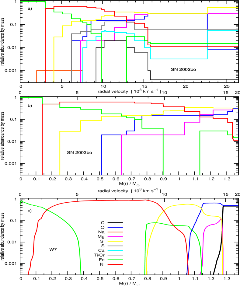
Figure 5: Upper panel: Abundance distribution of SN 2002bo including all elements. Middle: O, Mg, Si, Fe, and ⁵⁶Ni abundances in SN 2002bo. Lower panel: W7 deflagration model abundances (C, O, Mg, Si, Fe, ⁵⁶Ni).

The various steps above 7600 km s^-1 reflect the radii of the early-time spectra. Therefore, the distance between two abundance shells depends on the time interval between the two spectra. An additional shell above $22,700$ km s^-1 was inserted in order to account for high velocity material (Sect.4.1). Below 7600 km s^-1, where the abundances are derived from the nebular spectra, the radii of the shells are given by the density shells of the underlying W7 model. Since our models cover the entire SN ejecta, the total mass of each element can be calculated. These values are listed in Table 3. Different isotopes cannot be distinguished spectroscopically, so here the abundance of an element implies the sum of all isotopes, except for Fe.

Table 3: Total mass of elements spectroscopically confirmed in the ejecta of SN 2002bo and nucleosynthesis products of different SN Ia explosion models

	Ejected (Synthesized) Mass (M⊙)
Species	SN 2002bo	W7a	WDD1b	b30_3d_768c
C	$\la 0.002$	4.83E-02	5.42E-03	2.78E-01
O	0.110	1.43E-01	8.82E-02	3.39E-01
Na	0.001	6.32E-05	8.77E-05	8.65E-04
Mg	0.080	8.58E-03	7.69E-03	8.22E-03
Si	0.220	1.57E-01	2.74E-01	5.53E-02
S	0.067	8.70E-02	1.63E-01	2.74E-02
Ca	0 020	1.19E-02	3.10E-02	3.61E-03
Ti	0.003	3.43E-04	1.13E-03	8.98E-05
Cr	0.003	8.48E-03	2.05E-02	3.19E-03
Fe∗	0.360	1.63E-01	1.08E-01	1.13E-01
56Ni∗∗	0.520	5.86E-01	5.64E-01	4.18E-01
Ni∗∗∗	n.a.	1.26E-01	3.82E-02	1.06E-01

^∗Stable isotopes except for ⁵⁶Fe from ⁵⁶Co decay
^∗∗Isotopes from the ⁵⁶Ni $\rightarrow$ ⁵⁶Co $\rightarrow$ ⁵⁶Fe decay chain
^∗∗∗Stable isotopes ⁵⁸Ni, ⁶⁰Ni, ⁶¹Ni, ⁶²Ni, and ⁶⁴Ni
${}^{a}\,$Nomoto et al. (1984)
${}^{b}\,$Iwamoto et al. (1999)
${}^{c}\,$Travaglio et al. (2004)

Since the progenitor WD is supposed to be composed of C and O, the abundances of these two elements in the SN ejecta indirectly indicate the extent of burning. Interestingly, no sign of C can be seen in the spectra of SN 2002bo. The most prominent C lines in the optical and NIR wavelength bands are C ii 6579 Å and C ii 7231 Å. Neither line can be detected, at any epoch. Benetti et al. (2004) suggested an upper limit of the C abundance of 3% at $v>25,000$ km s^-1 based on models of the optical spectra. This upper limit corresponds to a total mass of $\la 2\times 10^{-3}$ M_⊙. Since no C lines are detected in the spectra, the C abundance in this analysis is set to zero.

The other progenitor element, O, dominates the ejecta between $15,500$ km s^-1 and $22,700$ km s^-1. In the outermost layers the abundance of Si is higher than that of O. In deeper layers the O abundance decreases, and no O can be found below 6000 km s^-1. Altogether we detect $\sim 0.11$ M_⊙ of O in SN 2002bo.

The group of IME includes Na, Mg, Si, S and Ca. Except for Na, they all show rather high abundances at high velocities. Na itself is located above the Fe core and out to $\sim 8500$ km s^-1, with a low abundance.

Mg is enhanced in SN 2002bo. A total mass of $\sim 0.08$ M_⊙ is derived from the modelling. The bulk of Mg is at $v>12,000$ km s^-1, with relative mass abundances between 20% and 30%. This is necessary to fit the deep 4481 Å absorption in the early phase, as discussed in Section 4. Below $\sim 15,000$ km s^-1 the Mg abundance decreases steadily, and no Mg is detected below 7300 km s^-1.

The Si abundance has a similar behaviour as Mg. However, the increase of the abundance at high velocity is more pronounced. The outermost shell ($v>22,700$ km s^-1) contains 52% of Si in order to account for the blue wing absorption of the various Si ii features. In the region between $11,450$ km s^-1 and $22,700$ km s^-1 Si is as abundant as O ($\sim 30$%). This is similar to the prediction of a model like W7, although somewhat on the high side. Deeper in the ejecta the Si abundance is $\sim 15$% down to $\sim 6000$ km s^-1, and then it drops rapidly until it disappears below 4000 km s^-1. A total mass of $\sim 0.22$ M_⊙ is derived, which is more than in W7 but less than in the DD models. It must be emphasised that the Si abundance in the deepest layers can only be derived indirectly, since the only nebular lines of Si are in the IR, which is not available for SN 2002bo.

S behaves like Si, but with a lower abundance, and does not exhibit a rise in the outermost shell. It starts at 6% outside, increasing to $\sim 13$% between 12,900 and 10,200 km s^-1, and decreasing to $\sim 6$% before disappearing below $\sim 6000$ km s^-1. The total mass of S is $\sim 0.067$ M_⊙.

Ca completes the set of IME that can be detected in SN 2002bo. This element is the best to study high velocity components, since its lines are the strongest. As discussed in Sect. 4, the Ca ii IR triplet lacks significant absorption in its blue wing. We tried to account for this using up to 20% Ca at intermediate and especially at high velocities. However, even with 100% Ca in the outermost layers it is impossible to fit the blue part of the line in the day –8 spectrum. On the other hand, the strong Ca ii 7291, 7324 Å nebular emission can be reproduced with a very small Ca abundance ($\sim 10^{-5}$ by mass). Therefore, a second iteration of the modelling of the early time spectra was performed using a significantly lower value for the Ca abundance. A satisfactory result was obtained for an abundance of 5.5% above $22,700$ km s^-1, decreasing to 0.3% in the next deeper shell and increasing again to 1% – 5.5% between $15,800$ and 7500 km s^-1. Below this velocity, the abundance is very small. A total 0.021 M_⊙ of Ca is estimated. The problem with the high velocity absorptions cannot be solved by a simple enhancement of the abundances, and may require scenarios like an increased density in the outer ejecta, possibly due to circumstellar interaction.

For Ti and Cr, which have a similar abundance trend, a total mass of $\sim 6\times 10^{-3}$ M_⊙ is derived. Although no individual lines of these species can be detected in the spectra, their line-blocking effect is necessary to shift UV and blue photons to longer wavelengths. The distribution of these elements peaks between $10,000$ and $15,000$ km s^-1, with values between 1 and 2%.

The abundance of ⁵⁶Ni includes plus both the ⁵⁶Co and ⁵⁶Fe that form in the decay chain. The relative abundances of these species change with time. ⁵⁶Ni dominates between about 3,000 and 10000 km s^-1, but its abundance never exceeds $\sim 60$%. Beyond this velocity the abundance decreases, dropping to $\la 1$% above $15,500$ km s^-1. We estimate the total ⁵⁶Ni mass synthesised to be $\sim 0.52$ M_⊙.

The abundance of just Ni includes all stable Ni nuclei (⁵⁸Ni, ⁶⁰Ni, ⁶¹Ni, ⁶²Ni, and ⁶⁴Ni), which are mostly located at the lowest velocities. The dominant isotope should be ⁵⁸Ni. The production of these species depends on the neutron excess during the burning regime. Especially in the W7 model stable Ni makes up a significant mass fraction of the inner ejecta. The synthetic spectra cannot differentiate between different isotopes.

The heading “Stable Fe” stands for the sum of all Fe isotopes (⁵⁴Fe, ⁵⁶Fe, ⁵⁷Fe, ⁵⁸Fe), except for the ⁵⁶Fe that is produced in the decay of ⁵⁶Co. A stable Fe core extends out to $\sim 3000$ km s^-1. Further out stable Fe decreases steadily, and it is absent in the velocity range from 9900 to $12,900$ km s^-1. This means that the ⁵⁶Fe from the decay of ⁵⁶Ni is sufficient to reproduce the spectra. Above this void region a small amount of stable Fe $(\sim 2$%) is again detected, extending to the highest velocities. The presence of stable Fe at high velocities is required because the outer layers are observed so early that only very little ⁵⁶Fe has been produced from ⁵⁶Ni. Altogether a total mass of 0.36 M_⊙ of stable Fe is measured.

We compared the derived abundance distribution of SN 2002bo with various explosion models. Figure 5b shows the distribution of the main elements (O, Mg, Si, stable Fe isotopes, and ⁵⁶Ni) versus $M(r)$. The 1-D deflagration model W7 (Nomoto et al., 1984) is shown in Fig. 5c for comparison. The radial distribution is very similar in the two plots. In both cases, the innermost part of the envelope is dominated by stable Fe isotopes. Above this is the ⁵⁶Ni-dominated region, and IME are located further out. Despite these similarities there are significant differences. In SN 2002bo the abundance pattern is shifted to higher velocities and the regions of Fe group elements, IME, and unburned material are not as well separated but rather more mixed. The inner stable Fe region is much larger. O is mixed down, Si and Mg extend to both lower and higher velocities than in W7 while ⁵⁶Ni and Fe are mixed to the outer regions. Finally, the region above $\sim 1.3$ M_⊙, which is completely unburned in W7, in SN 2002bo shows no trace of C and both IME and Fe-group elements are mixed outwards. In practice, in SN 2002bo we detect more stable Fe but no stable Ni (mostly ⁵⁸Ni in W7).

Since delayed detonation models burn high velocity regions to IME, they could possibly compare better to the abundance distribution of SN 2002bo. Hence we examined various detonation models, namely WDD1, WDD2, WDD3, CDD1, CDD2, and CDD3 (Iwamoto et al., 1999). Indeed, the occurrence of IME at high velocities in SN 2002bo is represented better by the DD models than by W7. However, O and the Fe-group elements show a very different behaviour, much closer to W7. In particular, the relative locations of Fe, Ni, IME, and unburned O is reproduced best by W7.

Therefore we may conclude that in the case of SN 2002bo W7 is the explosion model that fits best the abundance distribution derived from spectral synthesis calculations. However, if mixing effects are neglected it is difficult to reproduce the observed abundance distribution exactly. On the other hand, the analysis of a single object is not sufficient to constrain different explosion models. Abundance stratification analysis of several objects is necessary, and it is under way.

7 Bolometric light curve

Figure 6: uvoir light curve of SN 2002bo. The black dots represent the observed photometric points, the circles are the bolometric luminosity deduced from the synthetic spectra. Three models of the MC light curve code are shown using directly the abundances from the spectral analysis ($--$), the same abundances but with slightly increased ⁵⁶Ni mass (—), and W7 abundances with 0.5 M_⊙ of ⁵⁶Ni ($-\cdot-$).

In order to check the validity of our results independently, we used the abundance distribution obtained from the spectral modelling and computed a synthetic bolometric light curve, assuming that the density is given by W7 and using a grey MC light curve model (Cappellaro et al., 1997; Mazzali et al., 2001a). In Fig. 6 we compare the results with the bolometric light curve of SN 2002bo presented in Benetti et al. (2004).

The synthetic light curve reproduces the observed one successfully, and it performs exceedingly well in the early, rising branch. This is particularly exciting. In fact, the early light curve rise depends mostly on the mixing out of ⁵⁶Ni. A synthetic light curve computed with the unmixed W7 abundances and scaled to a ⁵⁶Ni mass of 0.5 M_⊙ shows a significantly later rise, which is in disagreement with the observations (Fig. 6). In that case, ⁵⁶Ni extends only up to $\sim 20,000$  km s^-1, so photons are trapped longer in the ejecta and the rise of the light curve is delayed. Evidently, abundance stratification is accurately determined by the spectral modelling, especially in the outer layers.

The model is less successful near the peak of the light curve. A slight modification of the abundances, with ⁵⁶Ni increased to about 0.56 M_⊙ and stable Fe decreased accordingly, yields a better fit of this phase. This is a small change, which does not affect the essence of our results.

8 The position of the photosphere and the reliability of the results

We mentioned that the velocities of IME lines in SN 2002bo are peculiarly high. Therefore, it is interesting to see how the velocities of the observed lines compare to the model calculations. Especially for the weaker lines, the photospheric radius should be a good estimate for the expansion velocities of the model line features. The evolution of the photospheric velocity is compared in Fig. 7 to the expansion velocities of Si ii 6355 Å, S ii 5640 Å, and Ca ii H&K, as measured from their minima (Benetti et al., 2004).

Figure 7: Evolution of the expansion velocities deduced from the minima of the Si ii 6355 Å, S ii 5640 Å, Ca ii H&K absorptions and the photospheric radius of the synthetic spectra, and the position of the photosphere in the light curve code.

The photosphere of SN 2002bo is at 15,800 km s^-1 on day $-12.9$, and recedes only by 700 km s^-1 until day $-11.0$. This slow decline phase accounts for trying to reproduce the high-velocity absorption features. After day $-11.0$, the decline is steeper (590 km s^-1 d^-1), and then it slows down again after maximum. The three lines exhibit a slightly different behaviour than the photosphere. Their velocities decrease more rapidly until day $\sim-8$ then they do afterwards. After maximum, the gradient is very similar to the photospheric one.

The S ii line has the lowest velocity, as may be expected since this is the weakest line that can be individually measured. After day $-8.0$ it forms well above the Montecarlo photosphere, but it matches the light curve photosphere up to abouty maximum.

The strong Si ii line declines at a slower rate, especially between day $-6.1$ and maximum. It is always significantly faster than the photospheric velocity, as can be expected since this strong line is formed well above the photosphere.

The Ca ii H&K line is very strong and it has the highest velocities. It evolves like the Si ii line, at higher velocities. However, the very high velocities measured in the earliest spectra ($\sim 25,000$ km s^-1) in both Ca ii H&K and Ca ii IR are probably not photospheric, but indicate the presence of a high-velocity component (Mazzali et al., 2005a, b).

The calculation of the light curve offers the opportunity to investigate the validity of the assumption of a sharp photosphere that is made in the MC code. The light curve code in fact computes $\gamma$-ray deposition as a function of depth and time, and estimates the position of a gray photosphere based on a simple opacity prescription. The photospheric velocity thus computed, also shown in Fig.6, follows closely the position determined by the MC spectrum synthesis code, and, even more closely, that traced by the velocity of the S ii line, which is sufficiently weak to be a good tracer of $v_{ph}$. We can now look at the fraction of the energy deposited above the photosphere as a function of time. This fraction reaches 10% between 1 and 2 days before maximum, it is $\sim 13$% at maximum and $\sim 25$% 6 days after maximum. These values indicate that up to about maximum the approximation of a sharp photosphere is acceptable, while in the spectrum at day $+5.9$ it is rather poor, and non-thermal excitation and ionisation effects that are not considered in the code may be relevant. Another test is the fraction of ⁵⁶Ni located above the photosphere. This is only $\sim 10$% at maximum and $\sim 20$% 6 days later, confirming the above result.

Fortunately, the depth of the zone explored between maximum light and the nebular spectra is quite small (between 7600 and 9000 km s^-1), since the photosphere recedes only slowly after maximum and then disappears. Nevertheless, abundances in that velocity range must be regarded as more uncertain than values both at higher velocities, where the MC code is more reliable, and at lower ones, which are treated with the nebular code.

9 Conclusions

We have derived the abundance stratification in the ejecta of the SN Ia 2002bo through a time series of spectral models. Synthetic spectra were computed for 13 epochs during the photospheric phase and 2 in the nebular phase.

The most important result is that although the abundances are not very different from those of a standard model such as W7, some mixing in abundance seems to have occurred. In particular, ⁵⁶Ni extends to higher velocities than in W7, and the IME are mixed both inwards and outwards. Some IME are present at the highest velocities, which may indicate interaction of the ejecta with a CSM or some asphericity in the explosion. Balancing this, O is mixed inwards. C is however not seen in the ejecta.

One possibility to produce a situation like that observed in SN 2002bo is multi-dimensional effects. Bubbles of burned material may rise to outer regions while fingers of unburned material sink to deeper layers. Unlike the case of global mixing, the direction from which the observer looks at the SN may be important. In the case of SN 2002bo one of these partially burned bubbles reaching out to high velocities may be in the line of sight, delivering the spectra and abundance distribution we observe. Had we looked from another position we might possibly have seen the missing C and less or no high-velocity components in the lines of IME (see, e.g. Kasen et al., 2004). In this context it would be interesting to verify whether multi-dimensional effects can account for the observed diversity in SNe Ia beyond the brightness-decline rate relation.

The investigation of the abundance stratification in a number of well-observed SNe Ia can contribute to our understanding of all these mechanisms.

AKNOWLEDGEMENTS

This work is supported in part by the European Union’s Human Potential Programme under contract HPRN-CT-2002-00303, ‘The Physics of Type Ia Supernovae.’ We would like to thank the Institute for Nuclear Theory at the University of Washington, Seattle, USA, for supporting a visit in the summer of 2004.

References

- Arnett (1969) Arnett W.D., 1969, Ap&SS, 5, 180
- Abbott & Lucy (1985) Abbott D.C., Lucy L.B., 1985, ApJ, 288, 679
- Benetti et al. (2004) Benetti S., Meikle P., Stehle M., et al., 2004, MNRAS, 348, 261
- Branch, et al. (1985) Branch D., Doggett, J.B., Nomoto, K., Thielemann, F.-K., 1985, ApJ, 294, 619
- Branch, Fisher & Nugent (1993) Branch D., Fisher A., Nugent P., 1993, AJ, 106, 2383
- Cacella et al. (2002) Cacella P., Hirose Y., Nakano S., Kushida Y., Kushida R., Li W.D., 2002, IAU Circ., 7847
- Cappellaro et al. (1997) Cappellaro E., Mazzali P.A., Benetti S., Danziger I.J., Turatto M., Della Valle M., Patat F., 1997, A&A, 328, 203
- Cappellaro, Evans & Turatto (1999) Cappellaro E., Evans R., Turatto M., 1999, A&A, 351, 459
- Gamezo et al. (2003) Gamezo V.N., Khokhlov A.M., Oran E.S., Chtchelkanova A.Y., Rosenberg R.O., 2003, Sci, 299, 77
- Han & Podsiadlowski (2004) Han Z., Podsiadlowski Ph., 2004, MNRAS, 350, 1301
- Harkness (1991) Harkness, R., 1991, in Supernova 1987A and other supernovae, eds. I.J. Danziger and K. Kjaer, p. 447 (ESO: Garching)
- Höflich & Khokhlov (1996) Höflich P., Khokhlov A.M., 1996, ApJ, 457, 500
- Iben & Tutukov (1984) Iben I.J., Tutukov A.V., 1984, ApJS, 54, 335
- Iwamoto et al. (1999) Iwamoto K., Brachwitz F., Nomoto K., Kishimoto N., Umeda H., Hix W.R., Thielemann F.-K., 1999, ApJSS, 125, 439
- Kasen et al. (2004) Kasen D., Nugent P., Thomas R.C., Wang L., 2004, ApJ, 610, 876
- Khokhlov (1991) Khokhlov A.M., 1991, A&A, 245, 114
- Lucy (1999) Lucy L.B., 1999, A&A, 345, 211
- Mazzali (2000) Mazzali P.A., 2000, A&A, 363, 705
- Mazzali & Lucy (1993) Mazzali P.A., Lucy L.B., 1993, A&A, 279, 447
- Mazzali et al. (1993) Mazzali P.A., Lucy L.B., Danziger I.J., Gouiffes C., Cappellaro E., Turatto M., 1993, A&A, 269, 423
- Mazzali, Danziger & Turatto (1995) Mazzali P.A., Danziger I.J., Turatto M., 1995, A&A, 297, 509
- Mazzali et al. (2001a) Mazzali P.A., Nomoto K., Cappellaro E., Nakamura T., Umeda H., Iwamoto K., 2001a, ApJ, 547, 988
- Mazzali et al. (2001b) Mazzali P.A., Nomoto K., Patat F., Maeda K., 2001b, ApJ, 559, 1047
- Mazzali et al. (2005a) Mazzali P.A., Benetti, S.; Stehle, M.; Branch, D.; Deng, J.; Maeda, K.; Nomoto, K.; Hamuy, M., 2005a, MNRAS, 357, 200
- Mazzali et al. (2005b) Mazzali P.A., et al., ApJ Letters, in press
- Niemeyer & Hillebrandt (1995) Niemeyer J.C., Hillebrandt W., 1995, ApJ, 452, 769
- Nomoto (1982) Nomoto K., 1982, ApJ, 257, 780
- Nomoto et al. (1984) Nomoto K., Thielemann F.-K., Yokoi K., 1984, ApJ, 286, 644
- Nugent et al. (1995) Nugent P., Phillips M., Baron E., Branch D., Hausschildt P., 1995, ApJ, 455, L147
- Pauldrach et al. (1997) Pauldrach, A. W. A.; Duschinger, M.; Mazzali, P. A.; Puls, J.; Lennon, M.; Miller, D. L., 1996, A&A, 312, 525
- Perlmutter et al. (1999) Perlmutter S., Aldering G., Goldhaber G., et al., 1999, ApJ, 517, 565
- Reinecke et al. (1999) Reinecke M., Hillebrandt W., Niemeyer J.C., Klein R., Gröbl A., 1999, A&A, 347, 724
- Reinecke, Hillebrandt & Niemeyer (2002) Reinecke M., Hillebrandt W., Niemeyer J.C., 2002, A&A, 391, 1167
- Riess et al. (1998) Riess A.G., Filippenko A.V., Challis P., et al., 1998, AJ, 116, 1009
- Travaglio et al. (2004) Travaglio C., Hillebrandt W., Reinecke M., Thielemann F.-K., 2004, A&A, in press
- Wang et al. (2003) Wang L., Baade D., Höflich P., et al., 2003, ApJ, 591, 1110
- Webbink (1984) Webbink R.F., 1984, ApJ, 277, 355
- Whelan & Iben (1973) Whelan J., Iben I.J., 1973, ApJ, 186, 1007
- Woosley & Weaver (1994) Woosley S.E., Weaver T.A., 1994, in: Audouze J., Bludman S., Mochovitch R., Zinn-Justin J., eds, Supernovae, Les Houches Session LIV, Elsevier, Amsterdam, p. 63
- Woosley, Axelrod & Weaver (1984) Woosley S.E., Axelrod T.S., Weaver T.A., 1984, in: Chiosi C., Renzini A., eds, Stellar Nucleosynthesis, Kluwer, Dordrecht, p. 263
- Woosley, Wunsch & Kuhlen (2004) Woosley S.E., Wunsch S., Kuhlen M., 2004, ApJ, 607, 921