The 2dF QSO Redshift Survey - XIV. Structure and evolution from the two-point correlation function.

Abstract

In this paper we present a clustering analysis of QSOs using over 20000 objects from the final catalogue of the 2dF QSO Redshift Survey (2QZ), measuring the redshift-space two-point correlation function, $\xi(s)$. When averaged over the redshift range $0.3<z<2.2$ we find that $\xi(s)$ is flat on small scales, steepening on scales above $\sim 25~{}h^{-1}~{}{\rm Mpc}$. In a WMAP/2dF cosmology ($\Omega_{\rm m}=0.27$, $\Omega_{\Lambda}=0.73$) we find a best fit power law with $s_{0}=5.48_{-0.48}^{+0.42}~{}h^{-1}~{}{\rm Mpc}$ and $\gamma=1.20\pm 0.10$ on scales $s=1$ to $25~{}h^{-1}~{}{\rm Mpc}$. We demonstrate that non-linear redshift-space distortions have a significant effect on the QSO $\xi(s)$ at scales less than $\sim 10~{}h^{-1}~{}{\rm Mpc}$. A cold dark matter model assuming WMAP/2dF cosmological parameters is a good description of the QSO $\xi(s)$ after accounting for non-linear clustering and redshift-space distortions, and allowing for a linear bias at the mean redshift of $b_{\rm Q}(z=1.35)=2.02\pm 0.07$.

We subdivide the 2QZ into 10 redshift intervals with effective redshifts from $z=0.53$ to $2.48$. We find a significant increase in clustering amplitude at high redshift in the WMAP/2dF cosmology. The QSO clustering amplitude increases with redshift such that the integrated correlation function, $\bar{\xi}(s)$, within $20~{}h^{-1}~{}{\rm Mpc}$ is $\bar{\xi}(20,z=0.53)=0.26\pm 0.08$ and $\bar{\xi}(20,z=2.48)=0.70\pm 0.17$. We derive the QSO bias and find it to be a strong function of redshift with $b_{\rm Q}(z=0.53)=1.13\pm 0.18$ and $b_{\rm Q}(z=2.48)=4.24\pm 0.53$. We use these bias values to derive the mean dark matter halo (DMH) mass occupied by the QSOs. At all redshifts 2QZ QSOs inhabit approximately the same mass DMHs with $M_{\rm DH}=(3.0\pm 1.6)\times 10^{12}h^{-1}M_{\odot}$, which is close to the characteristic mass in the Press-Schechter mass function, $M^{*}$, at $z=0$. These results imply that $L_{\rm Q}^{*}$ QSOs at $z\sim 0$ should be largely unbiased. If the relation between black hole (BH) mass and $M_{\rm DH}$ or host velocity dispersion does not evolve, then we find that the accretion efficiency ($L/L_{\rm Edd}$) for $L_{\rm Q}^{*}$ QSOs is approximately constant with redshift. Thus the fading of the QSO population from $z\sim 2$ to $\sim 0$ appears to be due to less massive BHs being active at low redshift. We apply different methods to estimate, $t_{\rm Q}$, the active lifetime of QSOs and constrain $t_{\rm Q}$ to be in the range $4\times 10^{6}-6\times 10^{8}$ years at $z\sim 2$.

We test for any luminosity dependence of QSO clustering by measuring $\xi(s)$ as a function of apparent magnitude (equivalent to luminosity relative to $L_{\rm Q}^{*}$). However, we find no significant evidence of luminosity dependent clustering from this data set.

1 Introduction

The question of how activity is triggered in the nucleus of galaxies is vital to answer if we wish to have a full understanding of the galaxy formation process. It appears that a large fraction of galaxies may have contained an active galactic nuclei (AGN) at some point in their history. When local galaxies are surveyed (including our own Milky Way) most show evidence of a super-massive black hole (BH) (e.g. Kormendy & Richstone 1995). The BHs tend to be found in dynamically hot systems (i.e. spheroids - elliptical galaxies or bulges), and the mass of the BHs is well correlated with the mass of the spheroid. The tightest correlation is found between BH mass, $M_{\rm BH}$, and spheroid velocity dispersion, $\sigma^{*}$ [Gebhardt et al.2000, Ferrarese & Merritt 2000]. At higher redshift it is not clear that this correlation holds, or indeed in general, how high redshift BHs relate to their host galaxies. However Shields et al. (2003) do suggest that the same $M_{\rm BH}-\sigma$ seems to be appropriate at high redshift.

It is the powerful evolution in luminosity of the AGN population which allows them to be readily observed to high redshift. Understanding this evolution goes hand-in-hand with our understanding of the relation between AGN and galaxies. Croom et al. (2004a) (which we will henceforth call Paper XII) find that optically selected QSOs are well described by so called ’pure luminosity evolution’ (PLE) with an exponential increase in the typical luminosity $L_{\rm Q}^{*}$ (e-folding time of $\sim 2$ Gyr) up to $z\sim 2$. Work at higher redshift (e.g. Fan et al. 2001) find that at $z\sim 4-6$ the number density of QSOs is much lower than at $z\sim 2$. The X-ray luminosity function (LF) appears to give a more complex picture [Ueda et al. 2003] but still shows the general trend of luminous AGN being more active, peaking at $z\sim 2-3$.

The question is then, how do we gain further information about the physical processes of QSO formation at high redshift? One approach is to attempt to directly image QSO host galaxies at high resolution [Kukula et al. 2001, Croom et al. 2004b]. These analyses seem to show that high redshift QSO hosts (at least for radio quiet sources) are no brighter than low redshift hosts, after accounting for only passive evolution of the stellar populations in the galaxies. QSO clustering measurements gives us an important second angle to study the hosts of QSOs, as the clustering amplitude can be considered as a surrogate for host mass or dark matter halo (DMH) mass, $M_{\rm DH}$. With large samples such as the 2dF QSO Redshift Survey (2QZ; Paper XII) it is possible to determine these host properties over a wide range in redshift. With an estimate of the host mass of these high redshift QSOs we can hope to determine whether the host mass vs. BH mass correlation at low redshift continues to high redshift. We can also attempt to predict the masses of the descendents of high redshift QSOs, and locate them in the local universe.

A number of authors (e.g. Martini & Weinberg 2001; Haiman & Hui 2001; Kauffmann & Haehnelt 2002) have constructed models for QSO evolution including clustering, and these need to be tested against accurate measurements. One parameter that can be derived from these models is a mean QSO lifetime, although the exact interpretation of this is rather model dependent.

As well as being used for the study of QSO formation/evolution, QSOs are also powerful probes of large-scale structure in their own right. The large volumes probed ($\sim 6\times 10^{9}$h^-3Mpc³ for the 2QZ in a universe with $\Omega_{\rm m}=0.3$ and $\Omega_{\Lambda}=0.7$) and high redshift sampled makes observations quite complementary with lower redshift galaxy observations and higher redshift CMB observations. A number of authors have attempted to detect high redshift QSO clustering [Osmer 1981, Shaver 1984, Shanks et al. 1987, Iovino & Shaver 1988, Andreani & Cristiani 1992, Mo & Fang 1993, Shanks & Boyle 1994, Croom & Shanks 1996, La Franca et al. 1998] and made some preliminary measurements of clustering evolution, but these have all been based on small samples of QSOs (typically a few hundred objects). At low redshift, there have also been a number of recent analysis. Grazian et al. (2004) find $s_{0}=8.6\pm 2~{}h^{-1}~{}{\rm Mpc}$ for a sample of bright, $B<15$, low redshift, $z<0.3$, QSOs. Miller et al. (2004) show that the AGN fraction in the SDSS galaxy survey is not dependent on environment, while Croom et al. (2004c) and Wake et al. (2004) show that low redshift, low luminosity AGN are clustered identically to non-active galaxies. The 2QZ provided the first large, deep sample with which to perform detailed clustering analysis at high redshift. Outram et al. (2003), Outram et al. (2004), Miller et al. (2004) and others have used the 2QZ to test cosmological models. The two-point correlation function (the subject of this paper) has been discussed by Croom et al. (2001a) for the preliminary, 10k, data release of the 2QZ [Croom et al. 2001b]. They found that the clustering of high redshift ($\bar{z}\simeq 1.5$) QSOs to be very similar to the clustering of typical galaxies at low redshift. They also found that the amplitude of clustering was approximately constant, or slightly increasing, with redshift.

For comparison to the high redshift QSO clustering results, there are now some measurements of galaxy clustering over similar redshift intervals. These suggest moderately high clustering amplitudes, generally not inconsistent with that measured for QSOs. E.g. Deep wide-field ($\sim$ few degrees) imaging surveys used to measure the angular correlation function of galaxies also suggest high clustering amplitudes [Postman et al. 1998]. However, various differences are found, depending on the magnitude limits and photometric bands used to define the samples. This is not surprising given that there is clearly evidence that galaxy clustering is a function of luminosity [Norberg et al. 2001]. This may also be the case for QSOs, although there has been no significant evidence for this to date [Croom et al. 2002]. At $z\sim 3$, galaxy surveys using the drop-out technique (e.g. Steidel et al. 1998) have found that $L\sim L^{*}$ galaxies also cluster similarly to local galaxies on scales $\lower 3.22916pt\hbox{$\sim$}\hbox to0.0pt{\hss\raise 1.1625pt\hbox{$<$}}10~{}h^{-1}~{}{\rm Mpc}$, with $r_{0}\simeq 4-6~{}h^{-1}~{}{\rm Mpc}$ for a cosmology with $\Omega_{\rm m}=0.3$ and $\Omega_{\Lambda}=0.7$ [Adelberger et al. 1998, Foucaud et al. 2003, Adelberger et al. 2003].

In this paper we use the final data relase of the 2QZ (Paper XII) to measure the QSO two-point correlation function over a wide range in redshift. The 2QZ is currently the best sample on which to perform this analysis, being by far the largest QSO sample with a high surface density ($\sim 35$ deg^-2). We focus in this paper on the redshift-space correlation function $\xi(s)$ and attempt to account for the effects of any $z$-space distortions. The real-space correlation function will be addressed in a further paper (da Ângela et al. in preparation), and the cross-correlation of QSOs in different luminosity intervals will be discussed by Loaring et al. (in preparation). In Section 2 we introduce the 2QZ sample and the techniques used in our analysis. In Section 3 we use mock QSO catalogues [Hoyle 2000] constructed from the large simulations to test the reliability of our corrections for variations in completeness in the 2QZ. The redshift averaged, redshift dependent and luminosity dependent 2QZ $\xi(s)$ measurements are presented in Sections 4, 5 and 6 respectively. We finally discuss our conclusions in Section 7.

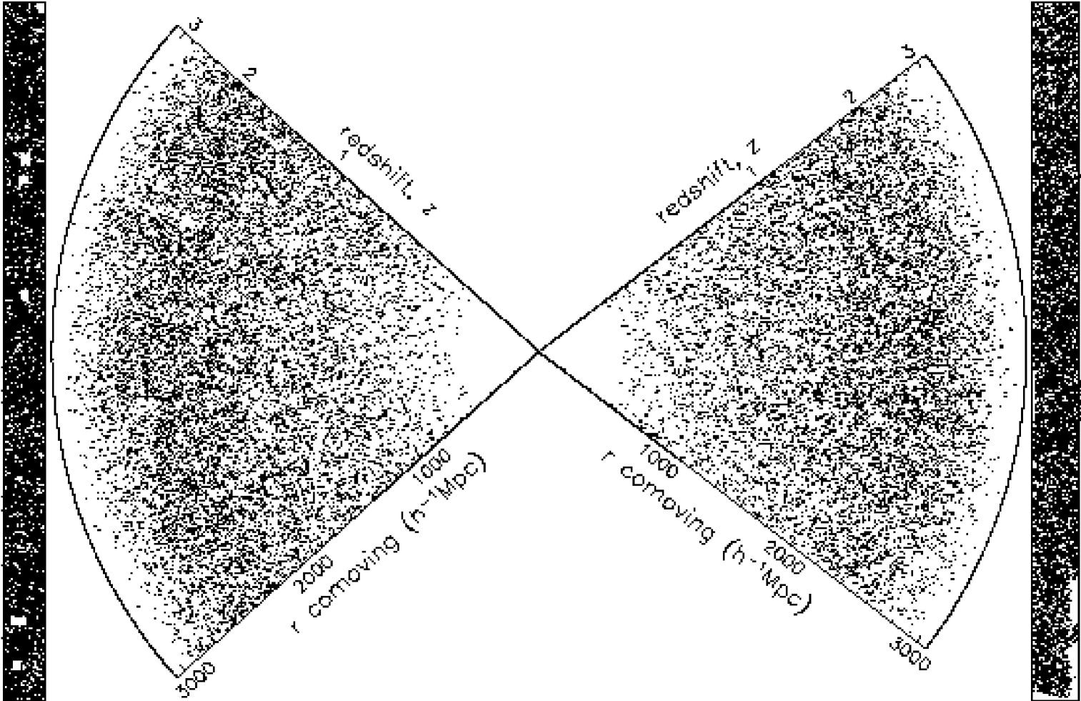
Figure 1: The distribution of 2QZ QSOs from the final catalogue. The SGP strip is on the left, the equatorial strip on the right. The rectangular regions show the distributions projected onto the sky. An EdS cosmology is assumed in calculating the comoving distances to each QSO.

2 Data and Techniques

2.1 The 2dF QSO Redshift Survey

There is a full description of the 2QZ in Paper XII. Briefly, the survey covers two $75^{\circ}\times 5^{\circ}$ strips, one passing across the South Galactic Cap centred on $\delta=-30^{\circ}$ (the SGP strip) and the other across the North Galactic Cap centred on $\delta=0^{\circ}$ (the NGP or equatorial strip). The SGP strip extends from $\alpha$ = 21^h40 to $\alpha$ = 3^h15 and the equatorial strip from $\alpha$ = 9^h50 to $\alpha$ = 14^h50 (B1950). The total survey area is 721.6 deg², when allowance is made for regions of sky excised around bright stars.

2dF spectroscopic observations were carried out on colour selected targets in the magnitude range $18.25<b_{\rm J}<20.85$. This resulted in the discovery of 23338 QSOs at redshifts less than $z\sim 3$. In this paper we restrict our analysis to QSOs with quality 1 identifications (see Paper XII), that is 22655 QSOs. The distribution of QSOs in the final sample is shown in Fig. 1.

2.2 Correlation function estimates

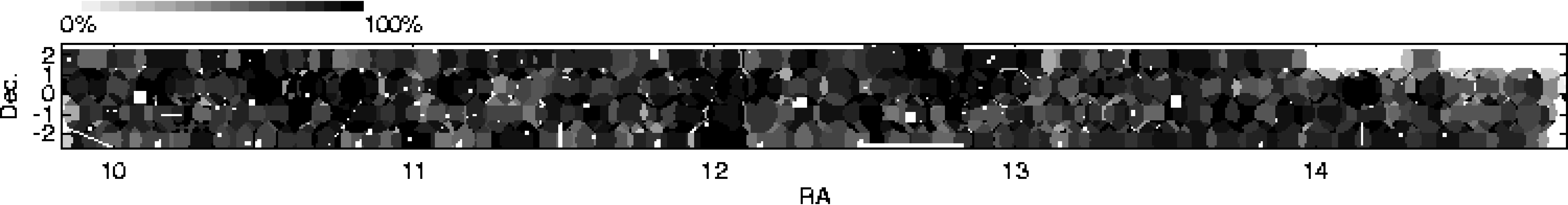
Figure 2: The completeness map of the 2QZ catalogue for the equatorial (top) and SGP (bottom) regions. The grey-scale indicates the percentage of all 2QZ targets that were both observed and positively identified (quality 1) over the two survey strips.

As the QSO correlation function, $\xi(s)$, probes high redshifts and large scales, the measured values are highly dependent on the assumed cosmology. In determining the comoving separation of pairs of QSOs we choose to calculate $\xi(s)$ for two representative cosmological models. The first uses the best fit cosmological parameters derived from WMAP, 2dFGRS and other data [Spergel et al. 2003, Percival et al. 2002] with $(\Omega_{\rm m}$,$\Omega_{\Lambda})=$ $(0.27,0.73)$, which we will call the WMAP/2dF cosmology. The second model assumed an Einstein-de Sitter cosmology with $(\Omega_{\rm m}$,$\Omega_{\Lambda})=$ $(1.0,0.0)$, which we denote as the EdS cosmology. We will quote distances in terms of $~{}h^{-1}~{}{\rm Mpc}$, where $h$ is the dimensionless Hubble constant such that $H_{0}=100h{\rm~{}km~{}s}^{-1}~{}{\rm Mpc}^{-1}$.

We have used the minimum variance estimator suggested by Landy & Szalay (1993) to calculate $\xi(s)$, where $s$ is the redshift-space (or $z$-space) separation of two QSOs (as opposed to $r$, the real-space separation). This estimator is

$$\xi(s)=\frac{QQ(s)-2QR(s)+RR(s)}{RR(s)},$$ (1)

where $QQ$, $QR$ and $RR$ are the number of QSO-QSO, QSO-random and random-random pairs counted at separation $s\pm\Delta s/2$. $QR$ and $RR$ are normalized to the total number of QSOs. The density of random points used was $50$ times the density of QSOs.

We calculate the errors on $\xi(s)$ using the Poisson estimate of

$$\Delta\xi(s)=\frac{1+\xi(s)}{\sqrt{QQ(s)}}.$$ (2)

At small scales, $\lower 3.22916pt\hbox{$\sim$}\hbox to0.0pt{\hss\raise 1.1625pt\hbox{$<$}}50~{}h^{-1}~{}{\rm Mpc}$, this estimate is accurate because each QSO pair is independent (i.e. the QSOs are not generally part of another pair at scales smaller than this). On larger scales the QSO pairs become more correlated and we use the approximation that $\Delta\xi(s)=[1+\xi(s)]/\sqrt{N_{\rm Q}}$, where $N_{\rm Q}$ is the total number of QSOs used in the analysis [Shanks & Boyle 1994, Croom & Shanks 1996]. We also derive field-to-field errors and compare these to the errors found in simulations. On small scales, $\lower 3.22916pt\hbox{$\sim$}\hbox to0.0pt{\hss\raise 1.1625pt\hbox{$<$}}2~{}h^{-1}~{}{\rm Mpc}$, the number of QSO-QSO pairs can be $\lower 3.22916pt\hbox{$\sim$}\hbox to0.0pt{\hss\raise 1.1625pt\hbox{$<$}}10$. In this case simple root-n errors (Eq. 2) do not give the correct upper and lower confidence limits for a Poisson distribution. We use the formulae of Gehrels (1986) to estimate the Poisson confidence intervals for one-sided 84% upper and lower bounds (corresponding to $1\sigma$ for Gaussian statistics). These errors are applied to our data for $QQ(s)<20$. Above this number of pairs root-n errors adequately describe the Poisson distribution.

In our analysis below we will also use the integrated correlation function out to some pre-determined radius as a measure of clustering amplitude. This is commonly denoted by $\bar{\xi}$, where

$$\bar{\xi}(s_{\rm max})=\frac{3}{s_{\rm max}^{3}}\int_{0}^{s_{\rm max}}\xi(x)x^{2}{\rm d}x.$$ (3)

As in Paper II we will generally take $s_{\rm max}=20~{}h^{-1}~{}{\rm Mpc}$ as this is on a large enough scale that linear theory should apply. The effect of $z$-space distortions due to small-scale peculiar velocities or redshift errors is also minimal on this scale.

2.3 Selection functions and incompleteness

The area of the survey is covered by a mosaic of 2dF pointings. These pointings overlap in order to obtain near complete coverage in all areas, including regions of high galaxy and QSO density. In order to take into account the variable completeness between 2dF pointings, due to variations in observational conditions, we use a mask that specifies the completeness of each survey sector, where we define a sector as the unique intersection of a number of circular 2dF fields. These masks are fully discussed in Paper XII. The completeness of each survey strip as a function of angular position on the sky is shown in Fig. 2. The distribution of random points used in our correlation analysis is constructed to have an identical distribution on the sky. In order to minimize the influence of low completeness fields, we restrict the analysis in this paper to sectors for which the spectroscopic completeness is at least 70 per cent. This results in a sample of 20686 QSOs in the redshift range $0.3<z<2.9$.

It is possible that on scales smaller than a 2dF field systematic variations in completeness may exist (e.g. see Paper XII). In order to test the consequence of these, detailed simulations have been carried out (see below). On larger scales small residual calibration errors in the relative magnitude zero-points of the UKST plates could add spurious structure. These are also assessed using simulations.

After generating random points according to the angular distribution specified by the completeness masks, we then assign a random redshift to each point. This random redshift is draw from a distribution defined by a polynomial fit to the observed $n(z)$ distribution (see Fig. 3a and Section 3.2.1 below).

As a direct test of the effectiveness of the above corrections, we also use random distributions generated by taking right ascensions (RAs) and declinations (Decs.) from the QSO catalogue itself. We then assign a redshift based on either the fitted $n(z)$ (as above; this we call the RA-Dec mixing method) or by assigning a random QSO redshift taken from the catalogue (the RA-Dec-z mixing method). These methods will mimic the 2QZ QSO angular distributions exactly, but with the effect of reducing the amount of structure measured (particularly on larger scales). We examine the reduction in large-scale power that these estimates cause below.

These two alternative methods also demonstrate that the QSO correlation function is not affected by the deficit of close ($<1^{\prime}$) pairs in the 2QZ. The deficit is due to the fact that the 2dF instrument cannot position two fibres closer than $\sim 30^{\prime\prime}$. It has in large part been alleviated by the overlapping field arrangement in the 2QZ strips, and the fact that the vast majority of QSO pairs which are close in angular position have very different redshifts. We therefore make no further corrections for this effect in our analysis.

Extinction by galactic dust will also imprint a signal on the angular distribution of the QSOs. Primarily this changes the effective magnitude limit in $b_{\rm J}$ by $A_{\rm b_{\rm J}}=4.035\times E(B-V)$ where we use the dust reddening $E(B-V)$ as a function of position calculated by Schlegel, Finkbeiner & Davis (1998). We then weight the random distribution according to the reduction in number density caused by the extinction such that

$$W_{\rm ext}(\alpha,\delta)=10^{-\beta A_{\rm b_{\rm J}}(\alpha,\delta)},$$ (4)

where $\beta$ is the slope of the QSO number counts at the magnitude limit of the survey. At $b_{\rm J}=20.85$, the magnitude limit of the 2QZ, the QSO number counts are flat, with $\beta\simeq 0.3$. Applying this correction we find that it only makes a significant difference to $\xi(s)$ on scales of $\sim 1000~{}h^{-1}~{}{\rm Mpc}$.

2.4 Making model comparisons to $\xi(s)$

Below we make comparisons of the data to a number of models, both simple functional forms (power laws) and more complex, physically motivated, models (e.g. cold dark matter; CDM). We use the maximum likelihood method to determine the best fit parameters. The likelihood estimator is based on the Poisson probability distribution function, so that

$$L=\prod_{i=1}^{N}\frac{e^{-\mu}\mu^{\nu}}{\nu!}$$ (5)

is the likelihood, where $\nu$ is the observed number of QSO-QSO pairs, $\mu$ is the expectation value for a given model and $N$ is the number of bins fitted. We fit the data with bins $\Delta\log(s)=0.1$, although we note that varying the bin size by a factor of two makes no noticeable difference to the resultant fit. In practice we minimize the function $S=-2{\rm ln}(L)$, and determine the errors from the distribution of $\Delta S$, where $\Delta S$ is assumed to be distributed as $\chi^{2}$. This procedure does not give us an absolute measurement of the goodness-of-fit for a particular model. We therefore also derive a value of $\chi^{2}$ for each model fit in order to confirm that it is a reasonable description of the data. In particular this is appropriate when fitting on moderate to large scales ($\lower 3.22916pt\hbox{$\sim$}\hbox to0.0pt{\hss\raise 1.1625pt\hbox{$>$}}5~{}h^{-1}~{}{\rm Mpc}$), where the pair counts are large enough that the Poisson errors are well described by Gaussian statistics.

3 Correlation function tests using mock QSO catalogues

3.1 Mock QSO catalogues

To test both our correlation function estimation methods and the effect of incompleteness we apply our analysis to mock QSO catalogues produced from the large Hubble Volume simulations of the Virgo Consortium [Frenk et al. 2000, Evrard et al. 2002]. In particular we make use of the $\Lambda$CDM Hubble Volume simulation where data on each particle has been output along the observer’s past light cone to mimic the 2QZ. The simulation contains $10^{9}$ particles in a cube that is $3000~{}h^{-1}~{}{\rm Mpc}$ on a side. The cosmological parameters of the simulation are $\Omega_{\rm b}=0.04$, $\Omega_{\rm CDM}=0.26$, $\Omega_{\Lambda}=0.7$, $H_{0}=70{\rm~{}km~{}s}^{-1}~{}{\rm Mpc}^{-1}$ and $\sigma_{8}=0.9$ (at $z=0$). The light cone data was output in a $75^{\circ}\times 15^{\circ}$ wedge oriented along the maximal diagonal of the cube, allowing the light cone to extend to a scale of $\sim 5000~{}h^{-1}~{}{\rm Mpc}$ ($z\sim 4$). These three slices are then split up into 3 largely independent $75^{\circ}\times 5^{\circ}$ slices, each one mimicing a single 2QZ strip. We note that there will be some correlation between the largest structures in the different simulation strips, however, it was not practical to generate simulations large enough to select many completely independent volumes.

In order to create realistic mock QSO catalogues, the mass particles are then biased to give a similar clustering amplitude to that observed in the 2QZ (based on the results of Croom et al. 2001a). The biasing prescription is based on that of Cole et al. (1998) (their model 2), but varying the parameters as a function of redshift to match the Croom et al. (2001a) results and using a cell size of $20~{}h^{-1}~{}{\rm Mpc}$ to determine the local density (Hoyle 2000). In our analysis below we consider mock catalogues with large numbers of biased particles ($\sim 100000$), almost a factor of 10 more than a single real 2QZ strip. This allows us to test for possible weak systematic affects. Full details of the Hubble Volume simulation are given by Hoyle (2000).

3.2 The effect of different correlation function estimates

Figure 3: QSO and simulation $n(z)$ distributions. a) The $n(z)$ distributions in the two 2QZ slices, SGP (solid line) and NGP (dotted line). The NGP has been renormalized to the number of QSOs in the SGP to aid comparison. Also shown is the 12th order polynomial fit to the combined $n(z)$ (dashed line). b) The $n(z)$ distribution of two Hubble Volume simulation slices each containing 12500 particles.

There are several issues involved with accurately determining the two-point correlation function. We will investigate each of these in turn.

3.2.1 Estimates of the QSO $n(z)$

The redshift distributions, $n(z)$, of the two 2QZ slices are shown in Fig. 3a. In order to directly compare the two, we renormalize the NGP $n(z)$ to contain the same total number as the SGP. The two strips have the same overall shape, however the we note that they appear to have more structure that the $n(z)$ distributions of the Hubble Volume simulations shown in Fig. 3b (note that the simulations have a cut off imposed at $z=2.2$). By examining the spatial distribution of the QSOs it is possible to see that the extra structure in the $n(z)$ is due to a number of weak large-scale structures. For example, the narrow peak in the NGP $n(z)$ at $z=1.5$ is due to a wall-like feature (top right of Fig. 1). We must therefore be careful not to remove any excess large-scale power by fitting the $n(z)$ on too fine a scale. A detailed discussion of structure on very large scales is given by Miller et al. (2004). In Fig. 3a we plot the polynomial fit (12th order) to the QSO $n(z)$ distribution used to generate the random distributions. Tests using higher and lower order polynomial fits (8th – 16th order) showed no significant differences between the resultant $\xi(s)$ estimates. We also found that different methods of fitting the $n(z)$ of the simulations (e.g. spline vs. polynomial) only caused differences at the $\sim 0.1$ per cent level, much smaller than the random errors in the measurements of $\xi(s)$ from the 2QZ.

3.2.2 Masks vs. randomizing

Figure 4: Comparison of masking (filled points) and RA-Dec mixing (open points) methods for the Hubble Volume simulations. Beneath each plot we show the ratio of the two correlation function measures, $\xi(s)_{\rm mask}/\xi(s)_{\rm mixing}$. a) $\xi(s)$ measured over a broad redshift range, $z=0.3-2.2$. There is no significant difference between the two estimates. b) $\xi(s)$ measured over a narrow redshift range, $z=1.35-1.70$. In this case the RA-Dec mixing method produces a correlation function which is $\sim 10-20$ per cent lower than the masking method.

Figure 5: Comparison of simulated correlation functions with (open points) and without (filled points) zero-point errors for a) the full redshift range and b) a narrow redshift range with $z=1.35-1.70$. The ratio of the points with and without zero-point errors, $\xi(s,\sigma_{\rm zp}=0.05)/\xi(s,\sigma_{\rm zp}=0.000)$, is shown below each plot.

Figure 6: Comparison of simulated correlation functions with (open points) and without (filled points) radially dependent incompleteness within 2dF fields for a) the full redshift range and b) a narrow redshift range with $z=1.35-1.70$. The ratio of the points with and without radial dependent incompleteness, $\xi(s)_{\rm rad}/\xi(s)$, is shown below each plot.

We next investigate differences between the methods described above to produce the random distributions. In particular, although the RA-Dec and RA-Dec-z mixing methods are effective at removing any variations in completeness, we also need to assess whether they also remove significant amounts of large-scale structure. To do this we determine the clustering in our simulations using these different methods. In Fig. 4 we show a comparison of the masking and RA-Dec mixing methods for a single Hubble Volume simulation slice. When the redshift range is broad (Fig. 4a) there is no significant difference between the two methods and the ratio of the two (bottom of Fig. 4a) is consistent with 1 at all scales. However if we take a narrower redshift interval, as in Fig. 4b, we do see significant depression of the clustering strength in the RA-Dec mixing method. This is because in a narrow redshift interval, the angular clustering of QSOs will be greater, due to the reduced amount of projection. Therefore we conclude that while the RA-Dec mixing method is a useful check of the clustering amplitude averaged over the full survey, it is not an accurate estimate when measuring QSO clustering evolution in narrow redshift slices. The same results were found for the RA-Dec-z mixing method.

3.3 The effect of the survey selection function and incompleteness

We now assess the effect of errors in the survey selection function on our estimates of $\xi(s)$. All these tests are carried out using the masking method. Errors in the zero-points of the UKST photographic plates are a possible source of excess large-scale power. To mimic this effect we divide the simulated survey strips into 15 $5^{\circ}\times 5^{\circ}$ regions and apply to each a Gaussian random zero-point error $\Delta m$, with a $\sigma=0.05$ mag. We then modulate the density of sources in that region by a factor of $10^{-0.3\Delta m}$, as the faint end slope of the QSO number counts is $\sim 0.3$. This equates to an error in the QSO density of 7 per cent for a zero-point error of 0.1 mag. With $\sigma=0.05$ the full range of zero-point errors used was $\simeq 0.15$ mag. We do not expect there to be real zero-point errors in the survey larger than this. A comparison of simulated correlation functions with and without zero-point errors is shown in Fig. 5. We see no systematic differences caused by the zero-point errors in either the full redshift interval (Fig. 5a), or narrower redshift intervals (Fig. 5b). We note that if the zero-point errors are increased (to values greater than the likely photometric errors in the survey) then significant differences can be seen. With $\sigma=0.1$ mag there are systematic offsets in $\xi(s)$ at the level of $\sim 1$ per cent which become significant on scales greater than $\sim 40~{}h^{-1}~{}{\rm Mpc}$.

Figure 7: The QSO $\xi(s)$ from the 2QZ using the masking method (filled points) and and RA-Dec mixing method (open points). A WMAP/2dF cosmology is assumed. Below we show the ratio of the two, $\xi(s)_{\rm mixing}/\xi(s)_{\rm mask}$.

Figure 8: The QSO $\xi(s)$ from the 2QZ, plotting the results from the SGP (filled points) and NGP (open points) separately. A WMAP/2dF cosmology is assumed. Below we show the ratio of the two, $\xi(s)_{\rm NGP}/\xi(s)_{\rm SGP}$. Note that the scale of the ratio plot is broader than the previous similar plots.

Another possible cause of systematic errors in $\xi(s)$ is the variations in completeness within 2dF fields. These can be caused by systematic errors in astrometry or field rotation which will be worse at the edges of a field, or atmospheric refraction effects, if a field was observed at a different hour angle to that which it was configured for. Paper XII showed that although radially dependent completeness is noticeable when observations of many individual fields are averaged together, if the overlap between fields and repeat observations are taken into account there is no systematic decline in completeness towards the edge of 2dF fields. In order to confirm that completeness variations within 2dF fields will not impact on our clustering analysis we perform detailed tests. We first position our 2dF field centres along the simulation strips, and then apply spectroscopic completenesses selected randomly from the actual field completenesses found in the survey. A mask is also generated to correct for this variable incompleteness. We then modulate the completeness within each simulated 2dF field such that it mimics the radial decrease seen in Paper XII (filled points in their Fig. 18). We then calculated $\xi(s)$ from these simulations, using a completeness mask which corrects for all effects apart from the variation in completeness within the 2dF fields. This is a worst case scenario, as in the simulations we allocate an object to only one field, and then derive the radial completeness variation from the centre of that field. In the actual survey, objects without IDs could be observed in overlapping fields. We compare the results to $\xi(s)$ measured without the radial completeness variations in Fig. 6. We find that the radial completeness variations have no significant impact on $\xi(s)$ for either the whole redshift range or in narrower redshift intervals. We also determine the effect of radial incompleteness on $\bar{\xi}(s)$ in narrow redshift intervals (which is used extensively in Section 5). The radial incompleteness typically only changes $\bar{\xi}(s)$ by $2-5$ per cent, with the worst case being 10 per cent. Given that the radial selection model is a worst case scenario, and that the measurement errors in $\bar{\xi}(s)$ are at least 20 per cent, any radial dependence of completeness within 2dF fields will not impact on our conclusions presented below.

4 The redshift averaged QSO correlation function

Figure 9: The QSO $\xi(s)$ from the 2QZ on scales $0-2000~{}h^{-1}~{}{\rm Mpc}$, plotted on a linear scale. Error bars are derived from the field-to-field variance between six sub-samples of the data set.

The above simulations confirm that our methods of correlation analysis, and any residual systematic errors in the 2QZ should not significantly bias our estimates of $\xi(s)$. We now present the results of applying our correlation analysis to the final 2QZ sample, beginning with $\xi(s)$ averaged over the redshift range $0.3<z<2.2$, for the most part, assuming a WMAP/2dF cosmology. We note that here we restrict the redshift range to regions of high completeness, and do not include QSOs above $z=2.2$. This is because the mean QSO colours move progressively further into the stellar locus above this redshift making the sample increasingly sensitive to small systematic errors in selection. This sample contains 18066 QSOs and has a mean redshift of $\bar{z}=1.35$.

4.1 Results

We first plot a comparison between the masking method and the RA-Dec mixing method for the redshift averaged QSO $\xi(s)$. This is shown in Fig. 7. Note that we only plot $\xi(s)$ on scales greater than $1~{}h^{-1}~{}{\rm Mpc}$ as we find no QSO-QSO pairs on scales smaller than this (in a WMAP/2dF cosmology). Also, for any other bins without QSO-QSO pairs we plot a point on the bottom x-axis without an error bar. We see that on all scales the two estimates are consistent within the Poisson measurement errors. There is some indication that the RA-Dec mixing method is slightly systematically lower than the mask method on scales $>20~{}h^{-1}~{}{\rm Mpc}$, which could be an indication of a weak systematic error in the mask method, but this is not a significant deviation. Given the consistency of the two methods, unless we state so explicitly, we will use the mask method for all of our $\xi(s)$ estimates.

Figure 10: The QSO $\xi(s)$ from the 2QZ (filled points) compared to the best fit power laws over a range of scales: $s=1-100~{}h^{-1}~{}{\rm Mpc}$ (solid line) and a) $s=1-25~{}h^{-1}~{}{\rm Mpc}$ for a WMAP/2dF cosmology or b) $s=1-10~{}h^{-1}~{}{\rm Mpc}$ for an EdS cosmology (dotted lines).

In a second check of the consistency of our results we plot a comparison of the measured $\xi(s)$ in each of the NGP and SGP strips (Fig. 8). Although, the $\xi(s)$ measured from the two strips is in broad agreement, the NGP strip shows slightly stronger clustering on scales $>20~{}h^{-1}~{}{\rm Mpc}$. Comparing the estimates of $\bar{\xi}(s)$ on different scales in the two strips we find that they are consistent ($0.9\sigma$, $1.3\sigma$ and $0.6\sigma$ differences for $s=20$, 30 and $50~{}h^{-1}~{}{\rm Mpc}$ respectively).

The large volume probed by the 2QZ allows $\xi(s)$ to be probed on very large scales, in excess of $\sim 1000~{}h^{-1}~{}{\rm Mpc}$. Most models do not predict any signal in $\xi(s)$ at large scales, however, there have been some claims of features in the QSO $\xi(s)$ (including using data from the 2QZ). E.g. Roukema, Mamon & Bajtlik (2002) claimed to see several features, including a positive feature at the level of $\sim 4$ per cent on a scale of $\sim 240~{}h^{-1}~{}{\rm Mpc}$ in the $\xi(s)$ of $\sim 2300$ QSOs from the initial release of 2QZ catalogue [Croom et al. 2001b]. To test these claims we make an estimate of the 2QZ $\xi(s)$ to the maximum scales probed by the sample. The results of this are shown in Fig. 9 for the WMAP/2dF cosmology (Roukema et al. assume $\Omega_{\rm m}=0.3$ and $\Omega_{\Lambda}=0.7$, but our results are similar for both cosmologies). As Fig. 9 probes very large scales, where QSO pairs could be correlated, we determine errors by measuring the variance between six subs-regions of the full data set (three $5^{\circ}\times 25^{\circ}$ regions in each 2QZ strip). The errors plotted is the measured rms between the six subsamples divided by $\sqrt{6}$ to account for the greater volume of the full sample. We note that on the largest scales even these field-to-field errors will somewhat inaccurate. By comparing the QSO-QSO pair counts for the full region and the six sub-regions we find that at $\sim 200~{}h^{-1}~{}{\rm Mpc}$ $\sim 10$ per cent of pairs come from correlations between different sub-regions. By $\sim 1000~{}h^{-1}~{}{\rm Mpc}$ this number has risen so that approximately half of all QSO-QSO pairs are from QSOs in different sub-regions. This means that on large scales there will be significant correlation between the sub-regions, but the reduction of pairs in each sub-regions will also increase the Poisson noise.

There is little evidence of any strong deviation from zero on any scale larger that $\sim 100~{}h^{-1}~{}{\rm Mpc}$ and the QSO $\xi(s)$ is zero to within 0.5 per cent over a broad range of scales. One point (at $90~{}h^{-1}~{}{\rm Mpc}$) deviates from zero by $\sim 1$ per cent. There is no evidence for a feature at $\sim 240~{}h^{-1}~{}{\rm Mpc}$. At various different scales there are some points that are greater than $1\sigma$ from zero. A $\chi^{2}$ test comparing the data to $\xi(s)=0$ at $s=100-1000~{}h^{-1}~{}{\rm Mpc}$ gives $\chi^{2}=76.1$ with 45 degrees of freedom (dof), which implies significant deviations at the 99.7 per cent level. The rms scatter over this scale range is $\pm 0.002$. The level of deviations away from zero at large scales is so small that we cannot be confident that they are real features and not due to low level residual systematics. However, residual systematic effects at this level will not affect any of our conclusions and we can have confidence that the masks used to define the selection function are removing structure not due to QSO clustering.

4.2 Fitting models to the QSO $\xi(s)$

Table 1: The results of power law fits to the 2QZ $\xi(s)$ averaged over the redshift range $0.3<z<2.2$. Model fits assuming a power law in $z$-space [$(s/s_{0})^{-\gamma}$] and a power law in real-space [$(r/r_{0})^{-\gamma}$] are presented (the second for a WMAP/2dF cosmology only). The real-space power law is corrected for the effects of linear and non-linear $z$-space distortion. We list the cosmology assumed, the scales fit over, the best fit parameters and associated errors, the measured $\chi^{2}$ values, number of dof, $\nu$ and probability of acceptance, $P(<\chi^{2})$.

Model	$\Omega_{\rm m}$,$\Omega_{\Lambda}$	$s_{\rm min}$,$s_{\rm max}$	$s_{0}$/$r_{0}$	$\gamma$	$\chi^{2}$	$\nu$	$P(<\chi^{2})$
$(s/s_{0})^{-\gamma}$	0.27,0.73	1.0,100.0	$5.55_{-0.29}^{+0.29}$	$1.633_{-0.054}^{+0.054}$	37.7	18	4.6e-3
$(s/s_{0})^{-\gamma}$	0.27,0.73	1.0,25.0	$5.48_{-0.48}^{+0.42}$	$1.20_{-0.10}^{+0.10}$	8.1	12	7.8e-1
$(s/s_{0})^{-\gamma}$	1.00,0.00	1.0,100.0	$3.89_{-0.18}^{+0.18}$	$1.713_{-0.052}^{+0.052}$	42.6	18	9.2e-4
$(s/s_{0})^{-\gamma}$	1.00,0.00	1.0,10.0	$3.88_{-0.53}^{+0.43}$	$0.86_{-0.17}^{+0.16}$	5.6	8	7.0e-1
$(r/r_{0})^{-\gamma}$	0.27,0.73	1.0,100.0	$5.81_{-0.29}^{+0.29}$	$1.866_{-0.060}^{+0.060}$	20.4	18	3.1e-1
$(r/r_{0})^{-\gamma}$	0.27,0.73	1.0,25.0	$5.84_{-0.33}^{+0.33}$	$1.647_{-0.047}^{+0.047}$	7.2	12	8.4e-1

We now attempt to fit a variety of models to the data. The simplest model traditionally fitted to correlation function estimates is a power law of the form

$$\xi(s)=\left(\frac{s}{s_{0}}\right)^{-\gamma},$$ (6)

where $s_{0}$ is the comoving correlation length, in units of $~{}h^{-1}~{}{\rm Mpc}$. We first fit a power law over the full range of scales where significant clustering is detected, from 1 to $100~{}h^{-1}~{}{\rm Mpc}$, using the maximum likelihood technique. For the WMAP/2dF cosmology, this resulted in best fit parameters $(s_{0},\gamma)=(5.55\pm 0.29,1.633\pm 0.054)$, however this fit is unacceptable at the 99.5 per cent level (see Table LABEL:tab:fitpowpar). This best fit power law (solid line) is compared to the data in Fig. 10a and it can be seen that the data are flatter on small scales and steeper on large scales than model. We then vary the maximum scale that we fit. Only by reducing this to $\sim 25~{}h^{-1}~{}{\rm Mpc}$ is an acceptable power law fit achieved. Over the range $1-25~{}h^{-1}~{}{\rm Mpc}$ we find best fit values $(s_{0},\gamma)=(5.48_{-0.48}^{+0.42},1.20_{-0.10}^{+0.10})$. The power law slope is significantly flatter when the fit is performed on these smaller scales, but the scale length, $s_{0}$ is largely unaffected. This shows that the shape of the QSO $\xi(s)$ changes with scale and does not follow a single pure power law, but steepens at large scales. We also fit similar power law models to $\xi(s)$ estimated assuming an EdS cosmology. Over the range $s=1-100~{}h^{-1}~{}{\rm Mpc}$ we find $(s_{0},\gamma)=(3.89\pm 0.18,1.713\pm 0.052)$, but as for the WMAP/2dF cosmology, this is clearly rejected (at the 99.9 per cent level) (see Fig. 10b). As above, fitting on a more restricted range of scales allows acceptable fits. We find an acceptable power law fit on scales $s=1-10~{}h^{-1}~{}{\rm Mpc}$ with $(s_{0},\gamma)=(3.88_{-0.53}^{+0.43},0.86_{-0.17}^{+0.16})$ (see Fig. 10b). The apparent break in the QSO $\xi(s)$ is unsurprising given that we generally only expect power law clustering in the regime where clustering is non-linear. Similar breaks have been seen in the clustering of low redshift galaxies (e.g. Hawkins et al. 2003). On scales $\lower 3.22916pt\hbox{$\sim$}\hbox to0.0pt{\hss\raise 1.1625pt\hbox{$>$}}10~{}h^{-1}~{}{\rm Mpc}$ where $\xi(s)<1$ clustering should be close to linear. Other affects, such as $z$-space distortions could also distort the measured $\xi(s)$ away from a power law.

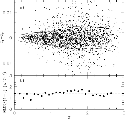
Figure 11: a) The difference between redshift measurements for repeated QSO observations in the 2QZ (using only quality 1 identifications and redshifts) as a function of mean redshift (points), also shown is the calculated rms in $\Delta z=0.1$ bins (solid lines). b) The rms redshift difference divided by $1+z$ as a function of mean redshift. The mean $\sigma_{z}/(1+z)$ is shown by the dashed line.

We assess the impact of $z$-space distortions on a power law. Small scale peculiar velocities will tend to reduce $\xi(s)$ on small scales. Both intrinsic peculiar velocities and redshift measurement errors will generate a similar effect. If due to intrinsic peculiar velocities, this should be best described by an exponential distribution [Ratcliffe et al. 1998, Hoyle et al. 2002, Hawkins et al. 2003] such that

$$f_{\rm exp}(w_{\rm z})=\frac{1}{\sqrt{2}\langle w_{\rm z}^{2}\rangle^{1/2}}\exp\left(-\sqrt{2}\frac{|w_{\rm z}|}{\langle w_{\rm z}^{2}\rangle^{1/2}}\right),$$ (7)

where $\langle w_{\rm z}^{2}\rangle^{1/2}$ is the rms pairwise line-of-sight velocity dispersion. If it is the redshift measurement errors which dominate, then the distribution may be better described by a Gaussian,

$$f_{\rm norm}(w_{\rm z})=\frac{1}{\langle w_{\rm z}^{2}\rangle^{1/2}\sqrt{2\pi}}\exp\left(-\frac{w_{\rm z}^{2}}{2\langle w_{\rm z}^{2}\rangle}\right).$$ (8)

The rms pairwise redshift error measured from repeat observations of 2QZ QSOs is given as $\sigma_{\rm z}=0.0027z$ in Paper XII. We have re-assessed this redshift error using the same data as Paper XII (Fig. 11) and find that a better estimate of the pairwise redshift error is $\sigma_{\rm z}=0.0014(1+z)$ (the dashed line in Fig. 11b). Thus the pairwise velocity error [$\delta v=c\delta z/(1+z)$] corresponding to this redshift error is $\delta v_{\rm z}=416{\rm~{}km~{}s}^{-1}$ largely independent of redshift. To this we need to add the intrinsic velocity dispersion of the QSOs, $\delta v_{\rm i}$. At low redshift the typical intrinsic galaxy pairwise velocity dispersion is $\simeq 500{\rm~{}km~{}s}^{-1}$ (e.g. Hawkins et al. 2003) at $z\simeq 0.15$. We note that Hawkins et al. did not include the factor of $1+z$ in Eq. 11 (see below). Correcting for this, the pairwise velocity is actually $\simeq 430{\rm~{}km~{}s}^{-1}$. It is uncertain whether this will decline with redshift. While the dark matter velocity dispersion should decline, as QSOs are biased tracers of large-scale structure, their pairwise velocity may not decline. Zhao, Jing & Borner (2002) predict that the pairwise velocity dispersion of Lyman-break galaxies at $z\sim 3$ could be $\sim 200-400{\rm~{}km~{}s}^{-1}$. Given the uncertainty in the evolution of $\delta v_{\rm i}$ we will assume a fixed value of $\simeq 430{\rm~{}km~{}s}^{-1}$ at all redshifts, noting that any evolution is likely to reduce this value. A final issue that needs to be considered is the velocity error due to intrinsic emission-line shifts in QSOs, $\delta v_{\rm l}$. The UV emission lines in QSO spectra typically show blue-shifts relative to their systemic velocity, this is particular so of lines such as CIV. Richards et al. (2002) demonstrated that the dispersion between centroids of CIV and MgII lines was $511{\rm~{}km~{}s}^{-1}$, while the dispersion between MgII and [OIII] was a somewhat smaller $269{\rm~{}km~{}s}^{-1}$. This dispersion will cause an extra dispersion in our redshift estimates which is not taken into account by the repeat observations (as they are repeats of the same QSO spectrum). Thus $\delta v_{\rm l}$ should take values in the range $200-450{\rm~{}km~{}s}^{-1}$ allowing for measurement errors [Richards et al. 2002]. Combining the three components of velocity dispersion together in quadrature results in $\langle w_{\rm z}^{2}\rangle^{1/2}\simeq 630-750{\rm~{}km~{}s}^{-1}$. In our analysis below we will assume a value of $690{\rm~{}km~{}s}^{-1}$ which lies in the middle of this range. As a combination of $\delta v_{\rm l}$ and $\delta v_{\rm z}$ dominates the total pairwise velocity dispersion, we use Eq. 8 to model the effects of $z$-space distortions on small scales. We note that other authors (e.g. Outram et al. 2004; Hoyle et al. 2002) used a similar value of $\langle w_{\rm z}^{2}\rangle^{1/2}\simeq 800{\rm~{}km~{}s}^{-1}$ (however they miss the factor of $1+z$ in Eq. 11 below).

Figure 12: a) model power law correlations functions demonstrating the effects of $z$-space distortions, assuming a real space $\xi(r)=(r/5)^{-1.8}$. In each case $\xi$ and $\bar{\xi}$ are plotted with $\bar{\xi}$ being the upper line. We show $\xi(r)$ (solid line), $\xi_{\rm lin}(s)$ (dotted line) and and $\xi_{\rm non-lin}(s)$ (dashed line). For the redshift-space distortion model we assume a WMAP/2dF cosmology, at a mean redshift of 1.35 with $\beta(z)=0.4$ and $\langle w_{\rm z}^{2}\rangle^{1/2}=690{\rm~{}km~{}s}^{-1}$. b) the ratio of different models comparing the ratios of $\xi_{\rm non-lin}(s)/\xi(r)$ (upper dashed line) and $\xi_{\rm non-lin}(s)/\xi_{\rm lin}(s)$ (upper dotted line). The other two dashed and dotted lines are the $\bar{\xi}$ equivalents. The two solid lines are set at 1.0 and at $(1+2\beta/3+\beta^{2}/5)=1.30$ for $\beta=0.4$.

We should also take into account the effect of linear $z$-space distortions. Kaiser (1987) showed that

$$\xi(s)=\xi(r)(1+\frac{2}{3}\beta+\frac{1}{5}\beta^{2}),$$ (9)

where $\xi(r)$ is the real-space correlation function and $\beta\simeq\Omega_{\rm m}^{0.6}/b$. More generally, $\xi(\sigma,\pi)$, the correlation function across (the $\sigma$ direction) and along (the $\pi$ direction) the line of sight is distorted, such that

$$\xi(\sigma,\pi)=\left[1+\frac{2(1-\gamma\mu^{2})}{3-\gamma}\beta+\frac{3-6\gamma\mu^{2}+\gamma(2+\gamma)\mu^{4}}{(3-\gamma)(5-\gamma)}\beta^{2}\right]\xi(r),$$ (10)

assuming that $\xi(r)$ is a power law [Matsubara & Suto 1996]. $\mu$ is the cosine of the angle between $r$ and $\pi$ (the distance along the line of sight), and $\gamma$ is slope of the power law. Then including the effects of non-linear $z$-space distortions, the full model for $\xi(\sigma,\pi)$ is given by

$$\xi(\sigma,\pi)=\int^{\infty}_{-\infty}\xi^{\prime}[\sigma,\pi-(1+z)w_{\rm z}/H(z)]f_{\rm norm}(w_{\rm z})\rm{d}w_{\rm z},$$ (11)

where $\xi^{\prime}[\sigma,\pi-(1+z)w_{\rm z}/H(z)]$ is given by Eq. 10, $f_{\rm norm}(w_{\rm z})$ is given by Eq. 8 and $H(z)$ is Hubble’s constant at a redshift, $z$. Finally, we carry out a spherical integral over the model $\xi(\sigma,\pi)$ to derive the model $\xi(s)$ which we then fit to the data. We note that there is an extra factor of $1+z$ in Eq. 11 compared to previous works (e.g. Hawkins et al. 2003; Hoyle et al. 2002). This is because the velocity dispersions are generally given in proper coordinates, rather than comoving coordinates. At low redshift this has a minimal affect, however, at high redshift this extra term boosts the effective scale corresponding to a given proper velocity by $1+z$ (in fact it approximately cancels out the increase of $H(z)$ with redshift, so that the proper velocity dispersion corresponds to a similar comoving scale at every redshift). It is therefore critical to incorporate this term. In this paper we are not specifically focussing on $\xi(\sigma,\pi)$ and $z$-space distortions, but only wish to determine their affect in shaping the measured $\xi(s)$. Detailed investigation of $\xi(\sigma,\pi)$ is discussed by da Ângela et al. (in preparation).

Figure 13: The QSO $\xi(s)$ from the 2QZ (filled points) compared to the best fit power law model incorporating the affects of linear and non-linear redshift-space distortions. A WMAP/2dF cosmology is assumed. The fits are carried out on scales $s=1-100~{}h^{-1}~{}{\rm Mpc}$ (solid line) and $s=1-25~{}h^{-1}~{}{\rm Mpc}$ (dotted line).

Estimates of the strength of $z$-space distortions via the QSO power spectrum have been made by Outram et al. (2004). They find that at $z=1.4$, the mean redshift of the sample used, $\beta=0.4\pm 0.1$. We assume this value for $\beta$ and a small-scale velocity dispersion of $690{\rm~{}km~{}s}^{-1}$. We then produce a grid of model real-space correlation functions which are adjusted for these $z$-space distortions and fitted to our observed $\xi(s)$ using the maximum likelihood technique.

In Fig. 12a we show a comparison of models with and without $z$-space distortions. Assuming a real-space correlation function of $\xi(r)=(r/5)^{-1.8}$ in a WMAP/2dF cosmology, and the above values of $\beta=0.4$ and $\langle w_{\rm z}^{2}\rangle^{1/2}=690{\rm~{}km~{}s}^{-1}$. The solid lines show the real-space $\xi(r)$ and $\bar{\xi}(r)$ (see Eq. 3). The model $\bar{\xi}(r)$ is a factor of $3/(3-\gamma)=2.5$ above $\xi(r)$. The dotted lines show the model $\xi(s)$ and $\bar{\xi}(s)$ for linear $z$-space distortions only ($\xi_{\rm lin}(s)$ i.e. $\beta=0.4$ and $\langle w_{\rm z}^{2}\rangle^{1/2}=0.0$), while the dashed lines show the full model with linear and non-linear $z$-space distortions ($\xi_{\rm non-lin}(s)$ i.e. $\beta=0.4$ and $\langle w_{\rm z}^{2}\rangle^{1/2}=690{\rm~{}km~{}s}^{-1}$). On scales less than $10~{}h^{-1}~{}{\rm Mpc}$ the non-linear $z$-space distortions cause a significant suppression of $\xi$. In Fig. 12b we plot the ratio of these various models. The dashed lines are $\xi_{\rm non-lin}(s)$ (top) and $\bar{\xi}_{\rm non-lin}(s)$ (bottom) divided by $\xi(r)$ and $\bar{\xi}(r)$ respectively. The dotted lines are $\xi_{\rm non-lin}(s)$ (top) and $\bar{\xi}_{\rm non-lin}(s)$ (bottom) divided by $\xi_{\rm lin}(s)$ and $\bar{\xi}_{\rm lin}(s)$ respectively. The solid lines are set at 1 and at $(1+2\beta/3+\beta^{2}/5)=1.30$ (for $\beta=0.4$). From this it can be seen that on scales $\sim 20-30~{}h^{-1}~{}{\rm Mpc}$ and larger the affect of non-linear $z$-space distortion is small, while the linear term affects $\xi$ on all scales. For the above power law, we find that $\bar{\xi}_{\rm non-lin}(s)/\bar{\xi}_{\rm lin}(s)=0.93$, 0.97 and 0.99 for $s=20$, 30 and $50~{}h^{-1}~{}{\rm Mpc}$ respectively.

To begin with we assume a power law model for $\xi(r)$ (Eq. 6). We generate a grid of models with different power law slopes ($\gamma$), and fit these models to the data using the maximum likelihood technique over the range $s=1-100~{}h^{-1}~{}{\rm Mpc}$. The resulting best fit model with $\beta=0.4$ and $\langle w_{\rm z}^{2}\rangle^{1/2}=690{\rm~{}km~{}s}^{-1}$ is shown by the solid line in Fig. 13. We find a power law slope of $\gamma=1.866\pm 0.060$ and a real-space scale length $r_{0}=5.81\pm 0.29~{}h^{-1}~{}{\rm Mpc}$. This provides an acceptable fit to the data with $\chi^{2}=20.4$ (18 dof) and an acceptance probability of 31 per cent. If we fit over a more restricted range of scales, noting that we expect deviations from a pure power law in real space on large scales, then we find best fit values of $\gamma=1.647\pm 0.047$ and $r_{0}=5.84\pm 0.33~{}h^{-1}~{}{\rm Mpc}$ for $s=1-25~{}h^{-1}~{}{\rm Mpc}$. Both fits are compared to the data in Fig. 13 (see also Table LABEL:tab:fitpowpar). When fitting on smaller scales the power law slope is flatter, however, $r_{0}$ is unchanged. It can be seen that the affect of small scale $z$-space distortions has a significant impact on scales less than $\sim 10~{}h^{-1}~{}{\rm Mpc}$.

Figure 14: The QSO $\xi(s)$ from the 2QZ (filled points) compared to a WMAP/2dF CDM model. The models shown are the linear real-space mass correlation function, $\xi_{\rho}(r)$ (short dashed line), the non-linear $\xi_{\rho}(r)$ (dotted line). The non-linear $\xi_{\rho}(r)$ scaled by the best fit bias value (long dashed line) and the non-linear mass correlation function corrected for $z$-space distortions, $\xi_{\rho}(s)$, scaled by the best fit bias (solid line).

More generally we should fit a model where the shape of $\xi(r)$ is governed by the underlying physics of the dark-matter distribution (e.g. CDM). In particular, Hamilton et al. (1991,1995) provide an analytic description of the generic linear CDM $\xi(r)$. The input parameters for the CDM model are taken from the now standard WMAP/2dF cosmological model [Spergel et al. 2003, Percival et al. 2002] with $\Omega_{\rm m}=0.27$, $\Omega_{\Lambda}=0.73$, $\Omega_{\rm b}=0.04$, $H_{0}=71{\rm~{}km~{}s}^{-1}~{}{\rm Mpc}^{-1}$, $\sigma_{8}=0.84$ (at $z=0$). We calculate the model $\xi(s)$ at the mean redshift of the 2QZ sample ($\bar{z}=1.35$), and correct for the affects of non-linear clustering [Hamilton et al. 1991, Jain et al. 1995]. Linear and non-linear $z$-space effects are accounted for as above, but using the more general prescription of Hamilton (1992) rather than Eq. 10 for the linear distortions. For the $z$-space distortions we assume $\beta=0.4$ and $\langle w_{\rm z}^{2}\rangle^{1/2}=690{\rm~{}km~{}s}^{-1}$. We then perform a maximum likelihood fit for a single parameter, a scale independent QSO bias, over the scale range $s=1-100~{}h^{-1}~{}{\rm Mpc}$. QSO bias is defined as

$$b_{\rm Q}(z)=\sqrt{\frac{\xi_{\rm Q}(r)}{\xi_{\rho}(r)}},$$ (12)

where $\xi_{\rm Q}(r)$ and $\xi_{\rho}(r)$ are the real-space QSO and mass correlation functions respectively. We note that our assumed value of $\beta$ includes an implicit assumption of QSO bias. If we substitute the $\xi_{\rm Q}(r)$ in Eq. 12 with that from Eq. 9 and solve the resultant quadratic in $b_{\rm Q}(z)$ we find that

$$b_{\rm Q}(z)=\sqrt{\frac{\xi_{\rm Q}(s)}{\xi_{\rho}(r)}-\frac{4\Omega_{\rm m}^{1.2}(z)}{45}}-\frac{\Omega_{\rm m}^{0.6}(z)}{3}.$$ (13)

This relation thus directly gives us the QSO bias at a redshift $z$, but is only strictly true if non-linear $z$-space distortions, which affect the shape of $\xi(s)$, are not present. The linear distortions do not affect the shape of $\xi(s)$ (this is exactly the case when there are no non-linear effects, and correct to first order in the presence of non-linear effects), so we fit a model $\xi_{\rho}(s)$ divided by $(1+2\beta/3+\beta^{2}/5)$ (using the same $\beta=0.4$ value used above) to obtain the ratio $\xi_{\rm Q}(s)/\xi_{\rho}(r)$ seen in Eq. 13. Assuming $\Omega_{\rm m}(z=0)=0.27$ [implying $\Omega_{\rm m}(z=1.35)=0.83$] we find a best fit QSO bias of $b_{\rm Q}(z=1.35)=2.02\pm 0.07$. This model is fully consistent with the data, with a $\chi^{2}=14.3$ from 19 dof (acceptable at the 76 per cent level, see the solid line in Fig. 14). The implied values of $\beta$ for this best fit bias is $\beta=0.44\pm 0.02$. This is close to our assumed value of $\beta=0.4$ and within the errors estimated by Outram et al. (2004) of $\pm 0.1$. To test the impact of making the $z$-space corrections to our model, we also fit the non-linear real space model to the data. This results in a best fit bias of $2.12\pm 0.09$ (long dashed line in Fig. 14), however, this is a slightly worse fit with a $\chi^{2}=25.2$ (19 dof) acceptable at the 15 per cent level. From Fig. 14 we see that the real-space model does not have a strong enough break at $\sim 10-20~{}h^{-1}~{}{\rm Mpc}$ to match the data. We conclude that the 2QZ QSO $\xi(s)$ averaged over redshift is fully consistent with the WMAP/2dF cosmology once allowance is made for the affects of $z$-space distortions.

4.3 Comparisons to other results

Figure 15: The QSO $\xi(s)$ from the 2QZ (filled points) compared to the the 2dFGRS $\xi(s)$ of Hawkins et al. (2003) (solid line, with $\pm 1\sigma$ errors shown by the dotted lines).

Figure 16: The QSO $\xi(s)$ from the 2QZ (filled points) compared to that for NVSS detected 2QZ QSOs (open points). The radio detected $\xi(s)$ uses broader bins of $\Delta\log(s)=0.2$.

The redshift averaged QSO $\xi(s)$ from the 2QZ is consistent with the current best fit cosmological model, after allowing for a linear bias $b_{\rm Q}(z=1.35)=2.02\pm 0.07$. We now compare our results to those from other estimates of $\xi(s)$. We find that there is very good agreement between the 2QZ $\xi(s)$ and 2dF Galaxy Redshift Survey (2dFGRS; Hawkins et al. 2003) $\xi(s)$ both in the shape and amplitude (see Fig. 15). We note that the 2QZ $\xi(s)$ may be slightly flatter than that of the 2dFGRS on small scales, as would be expected given the smaller influence of non-linear clustering at high redshift together with the larger impact of non-linear $z$-space distortions. However this is not significant. While the agreement in shape is not particularly surprising, the impressive match in amplitude is more surprising. This was also found in the preliminary 2QZ data release [Croom et al. 2001a]. Considering the evolution of clustering seen (see Section 5 below), this must be considered as something of a coincidence.

A number of authors have measured the spatial clustering of radio galaxies over a range of redshifts. Overzier et al. (2003) finds a real-space clustering scale-length $r_{0}=14\pm 3~{}h^{-1}~{}{\rm Mpc}$ at $z\sim 1$ for powerful radio galaxies, while weaker radio sources appear less clustered, with $r_{0}\sim 4-6~{}h^{-1}~{}{\rm Mpc}$. The clustering of 2QZ QSOs (which are largely radio quiet) is more similar to the radio weak sources. The 2QZ contains a small fraction of sources detected in the radio. There are 428 2QZ QSOs in the redshift range $0.3<z<2.2$ that are detected by the NRAO VLA Radio Survey (NVSS; Condon et al. 1998). The $\xi(s)$ we measure for this radio-detected population is shown in Fig. 16 (open circles). The small number of sources and their low surface density means that there is barely a detection of clustering, with only 2 QSO pairs detected vs. 1.15 expected at $s<20~{}h^{-1}~{}{\rm Mpc}$. The clustering of radio-detected QSOs in the 2QZ does not therefore impact on the clustering measurements of the full sample. There is a clear difference between the clustering of radio-quiet QSOs, as sampled by the 2QZ, and powerful radio galaxies, implying that radio galaxies must exist in more massive dark matter halos that radio-quiet QSOs.

The low redshift galaxy cluster correlation function has a much higher amplitude with $s_{0}$ typically $12-25~{}h^{-1}~{}{\rm Mpc}$ depending on the richness of the clusters [Bahcall et al. 2003]. There are few measurements of the cluster correlation length at high redshift. Gonzalex, Zaritsky & Wechsler (2002) find that approximately velocity dispersion limited samples of clusters at $z=0.35-0.575$ have similar clustering scale lengths to local clusters. For a WMAP/2dF cosmology, linear theory predicts that the amplitude of mass clustering between $z=1.35$ and $z=0$ will increase by a factor of $\simeq 3.4$, which is equivalent to an increase in $s_{0}$ by a factor of 2.0 (assuming $\gamma=-1.8$). Hence, even if QSO clustering at a mean redshift of $z=1.35$ evolved as strongly as linear theory evolution allows (making no allowance for evolution of bias), the descendents of objects that contained QSOs at $z\sim 1.4$ could not be clustered any more strongly than poor clusters at low redshift. Below we make a more detailed analysis of the evolution of QSO clustering to extend this analysis.

5 The evolution of QSO clustering

Table 2: 2QZ clustering results as a function of redshift for a WMAP/2dF cosmology. All fits are on scales $s=1-25~{}h^{-1}~{}{\rm Mpc}$. We list the redshift interval, and mean redshift, apparent magnitude and absolute magnitude (assuming $h=0.71$) for each bin together with the number of QSOs used. The best fit values of $s_{0}$ (in comoving units of $~{}h^{-1}~{}{\rm Mpc}$) and $\gamma$ are given with their $\chi^{2}$ values, number of dof, $\nu$ and probability of acceptance, $P(<\chi^{2})$. Lastly we also list the measured values of $\bar{\xi}(s)$ for $s=20$, 30 and $50~{}h^{-1}~{}{\rm Mpc}$.

$z$ interval	$\overline{z}$	$\overline{b}_{\rm J}$	$\overline{M}_{\rm b_{\rm J}}$	$N_{\rm Q}$	$s_{0}$	$\gamma$	$\chi^{2}$	$\nu$	$P(<\chi^{2})$	$\bar{\xi}(20)$	$\bar{\xi}(30)$	$\bar{\xi}(50)$
0.30,0.68	0.526	19.85	–22.16	2119	$5.73^{+0.79}_{-0.94}$	$-1.49^{+0.25}_{-0.25}$	15.9	10	1.02e-01	$0.263\pm 0.075$	$0.162\pm 0.041$	$0.071\pm 0.023$
0.68,0.92	0.804	19.93	–23.23	2067	$3.94^{+1.00}_{-0.98}$	$-1.15^{+0.24}_{-0.25}$	7.2	9	6.12e-01	$0.332\pm 0.085$	$0.118\pm 0.044$	$0.020\pm 0.022$
0.92,1.13	1.026	19.95	–23.86	2012	$4.76^{+0.97}_{-1.02}$	$-1.23^{+0.25}_{-0.25}$	6.7	9	6.71e-01	$0.353\pm 0.094$	$0.146\pm 0.048$	$0.063\pm 0.024$
1.13,1.32	1.225	19.97	–24.27	2066	$5.52^{+0.98}_{-1.00}$	$-1.04^{+0.25}_{-0.25}$	8.0	8	4.29e-01	$0.511\pm 0.100$	$0.226\pm 0.050$	$0.082\pm 0.024$
1.32,1.50	1.413	20.02	–24.57	2063	$5.28^{+0.98}_{-1.00}$	$-1.04^{+0.25}_{-0.25}$	3.4	7	8.51e-01	$0.452\pm 0.099$	$0.211\pm 0.050$	$0.064\pm 0.023$
1.50,1.66	1.579	20.02	–24.82	2011	$4.87^{+0.95}_{-1.02}$	$-0.94^{+0.25}_{-0.24}$	4.3	7	7.43e-01	$0.379\pm 0.096$	$0.205\pm 0.050$	$0.066\pm 0.024$
1.66,1.83	1.745	20.03	–25.06	2044	$6.25^{+0.83}_{-0.85}$	$-1.80^{+0.24}_{-0.25}$	3.5	10	9.66e-01	$0.321\pm 0.098$	$0.096\pm 0.049$	$0.045\pm 0.023$
1.83,2.02	1.921	20.05	–25.29	2020	$6.39^{+0.98}_{-1.00}$	$-1.09^{+0.25}_{-0.25}$	3.7	9	9.29e-01	$0.483\pm 0.111$	$0.260\pm 0.057$	$0.100\pm 0.026$
2.02,2.25	2.131	20.07	–25.51	2049	$8.00^{+0.99}_{-1.00}$	$-1.17^{+0.25}_{-0.25}$	5.6	9	7.82e-01	$0.607\pm 0.128$	$0.249\pm 0.063$	$0.074\pm 0.028$
2.25,2.90	2.475	20.09	–25.86	2235	$8.81^{+0.98}_{-1.01}$	$-1.24^{+0.25}_{-0.25}$	5.9	7	5.56e-01	$0.701\pm 0.174$	$0.289\pm 0.086$	$0.144\pm 0.039$

Above we have calculated $\xi(s)$ average over a broad redshift range. Under the assumption that QSO bias is largely scale independent (at least compared to the uncertainties in the clustering measurements) this should preserve the correct underlying shape of $\xi(s)$, particularly on large scales. However, according to the standard picture of gravitational growth of structure, the mass distribution should evolve with redshift. Croom et al. (2001a) showed that QSO clustering was constant or slightly increasing with redshift, with $s_{0}\simeq 5~{}h^{-1}~{}{\rm Mpc}$ up to $z\sim 2.5$. This demonstrated that QSOs must be biased tracers of the matter distribution, and that the amount of bias must evolve with redshift. Below we repeat this analysis with the final 2QZ data set, and discuss in detail the implications for QSO formation models. We will assume a WMAP/2dF cosmology unless stated otherwise.

5.1 Measurements of $\xi(s,z)$

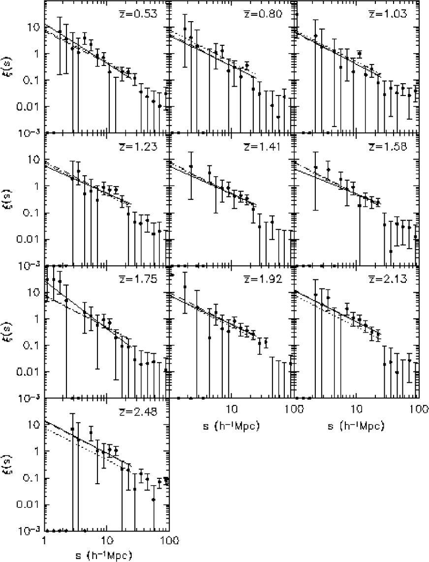
Figure 17: The QSO $\xi(s)$ from the 2QZ (filled points) as a function of redshift in 10 redshift bins containing approximately 2000 QSOs each. The best fit power law is shown in each case (solid line), as well as the best fit fixing $\gamma$ to be 1.20 (dashed lines). We also show the best fit power law for the full redshift range ($0.3<z<2.2$) for comparison (dotted line). A WMAP/2dF cosmology is assumed.

We split the QSOs up into 10 redshift intervals, such that there are approximately equal numbers of QSOs ($\sim 2000$) in each bin. Here we sample the redshift range $0.3<z<2.9$ and note that the final redshift interval $z=2.25-2.90$ could be affected by systematic variations in completeness on large scales. We perform the correlation analysis as described above on each of these sub-samples. In particular we use the mask method to correct for incompleteness, as the RA-Dec mixing method was shown to significantly suppress clustering measurements in narrow redshift intervals (see Section 3.2.2). We do, however, perform tests with the RA-Dec and RA-Dec-z mixing methods to confirm that there are no obvious unaccounted for systematic errors in our analysis. The resulting correlation functions are plotted in Fig. 17.

Figure 18: a) The evolution of $\bar{\xi}(s)$ for three different values of $s=20$, 30 and $50~{}h^{-1}~{}{\rm Mpc}$ (open circles, filled circles and open squares respectively). There is evidence for an increase in $\bar{\xi}$ with increasing redshift in all cases. b) The ratios of $\bar{\xi}$ as a function of redshift for $\bar{\xi}(20)/\bar{\xi}(30)$ (open circles) and $\bar{\xi}(50)/\bar{\xi}(30)$ (filled circles). The redshift averaged mean values for the ratios are indicated by the solid lines. The ratios are consistent with an unchanging shape for $\xi(s)$. The WMAP/2dF cosmology is assumed. Also plotted are the expected ratios for a CDM model with WMAP/2dF parameters (dotted lines).

In order to make quantitative measure of the clustering properties we calculate $\bar{\xi}(20)$ (Eq. 3) for each redshift interval. To test for any evidence of a change in shape of $\xi(s)$ we also calculate $\bar{\xi}$ using radii of $30$ and $50~{}h^{-1}~{}{\rm Mpc}$. The evolution of $\bar{\xi}$ is plotted in Fig. 18a using all three scales (the values are also listed in Table LABEL:tab:fitpar). In each case there is a general trend for $\bar{\xi}$ to increase with redshift. To assess the significance of the evolution we perform a Spearman rank correlation test on the $\bar{\xi}$ values. We find Spearman rank-order correlation coefficients, $\rho=0.721$, $0.648$ and $0.552$ for $\bar{\xi}$ determined at a radius of 20, 30 and $50~{}h^{-1}~{}{\rm Mpc}$ respectively. These correspond to correlation significances of $98.1$, $95.7$ and $90.2$ per cent. We note, of course, that as these are integral measures they are not independent of each other. The above test implies a significant correlation with redshift, however the data are still found to be consistent (via a $\chi^{2}$ test) with a single parameter model which is constant with redshift (only rejected at the 81, 77 and 75 per cent levels for $\bar{\xi}(20)$, $\bar{\xi}(30)$ and $\bar{\xi}(50)$ respectively).

In Fig. 18b we show the ratio of $\bar{\xi}(20)/\bar{\xi}(30)$ and $\bar{\xi}(50)/\bar{\xi}(30)$ to provide a simple test for any evidence of a change in the shape of $\xi(s)$ with redshift. These ratios are consistent with being constant over the full redshift range of the data set, suggesting that the shape of $\xi(s)$ does not change significantly with redshift. We also compare the $\bar{\xi}$ ratios to those assuming a CDM power spectrum in a WMAP/2dF cosmology (dotted lines in Fig. 18b). These are fully consistent with the observed ratios. In Fig. 19 we show the evolution of $\bar{\xi}(s)$ for an EdS cosmology. In this cosmology clustering is completely constant as a function of redshift, a Spearman rank correlation test shows no significant correlation.

Figure 19: The evolution of $\bar{\xi}(s)$ for three different values of $s=20$, 30 and $50~{}h^{-1}~{}{\rm Mpc}$ (open circles, filled circles and open squares respectively) in an EdS cosmology.

We next fit a simple power law model (Eq. 6). In Section 4.2 we find that a power law is an acceptable fit to the redshift averaged QSO $\xi(s)$ on scales $s=1-25~{}h^{-1}~{}{\rm Mpc}$. We therefore fit the data sub-divided into redshift intervals over the same range of scales. The best fit $s_{0}$ and $\gamma$ values are shown in Fig. 20 (and listed in Table LABEL:tab:fitpar). We carry out a Spearman rank test on both $s_{0}$ and $\gamma$ vs. redshift. For $s_{0}$ we find $\rho=0.770$ (99 per cent significant), while for $\gamma$ we find $\rho=-0.030$ (7 per cent significant). The measured values of $s_{0}$ are inconsistent with a constant value at 98 per cent significance. Given the lack of evolution in $\gamma$ we now fix its value and re-perform the fitting. For this we use the best fit power law slope of $\gamma=1.20$. The $s_{0}$ values derived are plotted in Fig. 20 (open points). These are similar to those found when allowing $\gamma$ to vary freely. A Spearman rank correlation test confirms that the correlation is still present with $\rho=0.842$ significant at the 99.8 per cent level.

Figure 20: a) The fitted values of $s_{0}$ with freely varying $\gamma$ (filled points) and fixed $\gamma$ (open points) as a function of redshift. b) The best fit values of $\gamma$ as a function of redshift. The dotted lines indicate the best fit values to the full redshift range. A WMAP/2dF cosmology is assumed.

Examining the highest redshift bin in Fig. 17 we see that there is significant signal at scales $\sim 70-100~{}h^{-1}~{}{\rm Mpc}$. This redshift interval at $2.25<z<2.90$ has a large variation in completeness with redshift, as the absorption due to the Lyman-$\alpha$ forest quickly moves the mean QSO colours into the stellar locus (see Paper XII). We do not need to calculate the absolute completeness in each redshift interval, as we rely on fitting to the observed shape of the QSO $n(z)$ relation. However, if this fit is not accurate enough over a given redshift interval, or there are systematic differences in the $n(z)$ covering different regions of the 2QZ survey, extra spurious large-scale structure could be added. We test for the presence of any such systematic affect by first calculating the $\xi(s,z)$ using RA-Dec-z mixing. This produces estimates of $\xi(s)$ which are systematically biased low (see Section 3.2.2), however any broad trends should still be present. We find that the highest redshift bin still has the largest best fit value of $s_{0}$ using these mixing methods. As a second test we calculate $\xi(s)$ for the $2.25<z<2.90$ interval by normalizing the total number and the redshift distribution of the random points within each UKST field. This would remove the affects of any UKST photometric zero-points errors or the differential affects of variability on completeness in different fields. The results of this analysis are indistinguishable from those using masking and the full 2QZ strips. While it is possible that this excess large-scale structure is still caused by systematic error, its size does not influence any of our main results below. Infact the final redshift bin could be completely ignored without changing our basic conclusions.

5.2 Comparison to simple models

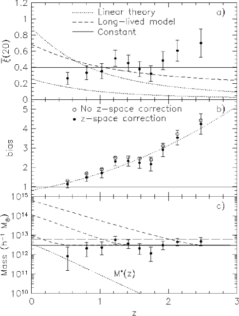
Figure 21: a) Our measurement of $\bar{\xi}(20)$ for 2QZ QSOs as a function of redshift (filled points). The data are compared to linear theory gravitational evolution (dotted lines) for two normalizations, one normalized to a WMAP/2dF cosmology (lower dotted line) and a second normalized to provide a ’best fit’ to the data points (upper dotted line). We also compare to the best fit for a constant $\bar{\xi}(20)$ (solid line) and a long-lived model (short dashed line). b) The QSO bias, $b_{\rm Q}(z)$ as a function of redshift derived from a comparison of $\bar{\xi}(20)$ for QSOs to that expected for the WMAP/2dF cosmology. The open points are the raw bias values [i.e. $\bar{\xi}_{\rm Q}(s)/\bar{\xi}_{\rho}(r)$] while the filled points with error bars are the values after making a consistent correction for $z$-space distortions. A simple empirical model is also shown (dotted line). c) The mean mass of DMHs containing QSOs derived from the measured bias (filled points). We also show the mean mass averaged over redshift (solid line) and the mean plus twice the rms of the points (long dashed line). $M^{*}(z)$, the characteristic mass which is just collapsing at a given redshift is denoted by a dotted line. The short dashed lines show the median expected growth in DMH mass from the mean DMH mass of QSO hosts at $z=0.53$, 1.41 and 2.48.

Following Paper II we test a number of simple models against the observed data. To be conservative we use the $\bar{\xi}(20)$ measurements, rather than the best fit $s_{0}$ values which are dependent on the range of scales fit and assumptions concerning the slope, $\gamma$. We note that removing the highest redshift point does not remove the detected correlation between $\bar{\xi}(20)$ and redshift, although it does reduce its significance ($\rho=0.617$, significant at the 92 per cent level). The significance of the correlations of $\bar{\xi}(30)$ and $\bar{\xi}(50)$ with redshift are also reduced removing when the highest redshift point is removed (to 85 and 69 per cent respectively).

We compare our results to the expected growth in density perturbations from linear theory, which should be applicable on the scales we are probing. For an EdS universe, the linear growth rate, $D(z)$, is given by $D(z)=1/(1+z)$, and for other cosmologies we use the accurate fitting formula of Carroll, Press & Turner (1992). In Fig. 21a we plot the measured $\bar{\xi}(20)$ for QSOs vs. linear theory models (dotted lines). We assume a CDM model with WMAP/2dF parameters. In this model the values of $\bar{\xi}(r,z=0)$ for the mass distribution are 0.254, 0.123 and 0.042 for $r=20$, 30 and $50~{}h^{-1}~{}{\rm Mpc}$ respectively. We plot two linear theory lines, the first (lower dotted line) assumes the above normalization given by WMAP/2dF, which is significantly below the points at all redshifts. The second (upper dotted line) is the linear theory model re-normalized by a constant bias to a ’best fit’ value for the data points. As in Croom et al. (2001a) we find linear theory evolution with a fixed bias to be in clear disagreement with the data (the probability of acceptance is formally $3.6\times 10^{-9}$). Assuming an EdS cosmology, we also get a rejection of QSOs following linear theory evolution (rejected at the 99.98 per cent level). We next fit the long-lived QSO model discussed by Croom et al. (2001a) which has the form

$$b_{\rm Q}(z)=1+[b_{\rm Q}(z=0)-1]/D(z).$$ (14)

This model is equivalent to assuming that QSOs have ages of order the Hubble time, and after formation at some arbitrarily high redshift subsequent evolution is governed by their motion within the gravitational potential [Fry 1996]. It is also equivalent to QSOs forming in density peaks above a constant threshold [Croom & Shanks 1996]. The best fit value of $b_{\rm Q}(z=0)=1.64\pm 0.05$ (short dashed lines in Fig. 21a), however, while Croom et al. (2001a) found this model was marginally acceptable in a cosmology with $\Omega_{\rm m}=0.3$ and $\Omega_{\Lambda}=0.7$ we find that the extra signal in the final 2QZ data set rejects the long-lived model at a significance level of 99.97 per cent in the WMAP/2dF cosmology. Fitting this model in the EdS Universe gives $b_{\rm Q}(z=0)=1.40\pm 0.04$, and is marginally acceptable (rejected at the 89 per cent level).

5.3 Bias, dark matter halo mass and the evolution of QSOs

Figure 22: The ratio of $\bar{\xi}_{\rm non-lin}(s)/\bar{\xi}_{\rm lin}(s)$ ($\bar{\xi}$ including and not including non-linear $z$-space distortions) as a function of redshift for $\langle w_{\rm z}^{2}\rangle^{1/2}=630$, 690 and $750{\rm~{}km~{}s}^{-1}$ (solid, dotted and dashed respectively) at scales $s=20$, 30 and $50~{}h^{-1}~{}{\rm Mpc}$ (bottom to top).

By assuming an underlying cosmological model we are able to convert the measured values of $\bar{\xi}$ to an effective bias by making comparisons to linear theory evolution. This allows us to directly determine QSO bias as a function of redshift. In doing so, we need to account for the affect of $z$-space distortions on the measured values of $\bar{\xi}(s)$. The non-linear $z$-space distortions have a small affect on the scales we are examining here (see Section 4.2). To determine their affect on $\bar{\xi}(s)$ we derive the ratio of $\bar{\xi}(s)$ with linear and non-linear $z$-space distortions to that including only the linear distortions, $\bar{\xi}_{\rm non-lin}(s)/\bar{\xi}_{\rm lin}(s)$. This is plotted for the CDM model with WMAP/2dF parameters as a function of redshift for $\langle w_{\rm z}^{2}\rangle^{1/2}=630$, 690 and $750{\rm~{}km~{}s}^{-1}$ in Fig. 22 (solid, dotted and dashed lines respectively). In constructing the models we assume values of $\beta$ that are consistent with the $\beta(z=1.4)=0.4\pm 0.1$ of Outram et al. (2004) and also account for the evolution of bias we find below. This assumption of $\beta$ only influences the shape of $\xi(\sigma,\pi)$ that is convolved with Eq. 8 to determine the non-linear $z$-space distortions. Varying the assumed $\beta$ within reasonable limits results in negligible difference in the $\bar{\xi}_{\rm non-lin}(s)/\bar{\xi}_{\rm lin}(s)$ ratio (less than 0.5 per cent). We plot the ratio for $s=20$, 30 and $50~{}h^{-1}~{}{\rm Mpc}$ (top to bottom) and see that even at $s=20~{}h^{-1}~{}{\rm Mpc}$ the worst correction is only 12 per cent. Assuming $\langle w_{\rm z}^{2}\rangle^{1/2}=690{\rm~{}km~{}s}^{-1}$, the range of reasonable values for $\langle w_{\rm z}^{2}\rangle^{1/2}$ results in a scatter of only $\sim 2$ per cent at $s=20~{}h^{-1}~{}{\rm Mpc}$ and less at larger scales. This is considerably smaller than the measurement errors in $\bar{\xi}$, and we therefore use the derived ratio for $\langle w_{\rm z}^{2}\rangle^{1/2}=690{\rm~{}km~{}s}^{-1}$ to correct our results for non-linear $z$-space affects (dotted lines in Fig. 22). Linear $z$-space distortions (Eq. 9) have a more significant affect, (e.g. a factor of $\sim 1.3$ at $z\sim 1.4$). We use Eq. 13 to self-consistently determine the QSO bias at a given redshift.

Table 3: The derived QSO bias, $b_{\rm Q}$ and DMH mass, $M_{\rm DH}$ as for 2QZ QSOs at a function of redshift in a WMAP/2dF cosmology. We also list the mean redshift and absolute magnitude of each redshift interval, as well as the value of $M_{\rm b_{\rm J}}^{*}$ derived from the polynomial evolution model of Paper XII and the space density of QSOs, $\Phi$, found by integrating the QSO luminosity function between the apparent magnitude limits of the 2QZ.

$\overline{z}$	$\overline{M}_{\rm b_{\rm J}}$	$M_{\rm b_{\rm J}}^{*}$	$\Phi$ $h^{3}{\rm Mpc}^{-3}$	$b_{\rm Q}$	$M_{\rm DH}$ $h^{-1}M_{\odot}$
0.526	–22.16	–23.24	$9.6\times 10^{-6}$	$1.13\pm 0.18$	$0.82_{-0.67}^{+1.55}\times 10^{12}$
0.804	–23.23	–23.94	$7.6\times 10^{-6}$	$1.49\pm 0.21$	$2.09_{-1.30}^{+2.18}\times 10^{12}$
1.026	–23.86	–24.41	$6.8\times 10^{-6}$	$1.71\pm 0.24$	$2.31_{-1.37}^{+2.23}\times 10^{12}$
1.225	–24.27	–24.78	$6.6\times 10^{-6}$	$2.31\pm 0.23$	$5.76_{-2.21}^{+2.90}\times 10^{12}$
1.413	–24.57	–25.07	$6.3\times 10^{-6}$	$2.32\pm 0.27$	$3.69_{-1.62}^{+2.24}\times 10^{12}$
1.579	–24.82	–25.29	$6.1\times 10^{-6}$	$2.24\pm 0.30$	$2.05_{-1.07}^{+1.61}\times 10^{12}$
1.745	–25.06	–25.47	$5.8\times 10^{-6}$	$2.17\pm 0.35$	$1.15_{-0.72}^{+1.24}\times 10^{12}$
1.921	–25.29	–25.61	$5.3\times 10^{-6}$	$2.91\pm 0.35$	$3.05_{-1.34}^{+1.85}\times 10^{12}$
2.131	–25.51	–25.72	$4.8\times 10^{-6}$	$3.53\pm 0.38$	$4.46_{-1.68}^{+2.20}\times 10^{12}$
2.475	–25.86	–25.76	$3.5\times 10^{-6}$	$4.24\pm 0.53$	$4.78_{-1.99}^{+2.68}\times 10^{12}$

Fig. 21b shows the derived bias of 2QZ QSOs as a function of redshift (filled points). The open points are the values found without accounting for $z$-space distortions. Here we see that QSO bias is strongly evolving with redshift, from $b_{\rm Q}(z=0.53)=1.13\pm 0.18$ to $b_{\rm Q}(z=2.48)=4.24\pm 0.53$ (see Table LABEL:tab:biasmass). A simple empirical description of the bias evolution found is

$$b_{\rm Q}(z)=(0.53\pm 0.19)+(0.289\pm 0.035)(1+z)^{2},$$ (15)

which is shown in Fig. 21b (dotted line). At $z\sim 0.5$ the value of $b_{\rm Q}$ is already close to 1, and a simple extrapolation of the trend observed would predict that the bias would at or below 1 at $z=0$. We note at this point that because of the apparent magnitude limit of the 2QZ, the mean absolute magnitude in each interval increases with redshift (see Table LABEL:tab:fitpar). However, the 2QZ selects QSOs that are close to $\sim L_{\rm Q}^{*}$ (the characteristic luminosity of the QSO optical luminosity function) at every redshift, and the space density of objects in each of the redshift slices is also approximately equal. Table LABEL:tab:biasmass lists the values of $M_{\rm b_{\rm J}}^{*}(z)$ assuming the polynomial evolution model of Paper XII (which is an uncertain extrapolation beyond $z=2.1$). Although the actual values of $M_{\rm b_{\rm J}}^{*}(z)$ should be used with caution as the fitted value of $M_{\rm b_{\rm J}}^{*}(0)$ is correlated with the bright and faint end slopes of the LF, it can be seen that there is little change in the relative difference between $M_{\rm b_{\rm J}}^{*}(z)$ and $\overline{M}_{\rm b_{\rm J}}(z)$ (less than 1 mag at $z<2.2$). Also listed is the space density found by integrating the observed luminosity function over the apparent magnitude range of the 2QZ for each redshift. Between $z=0.5$ and $z=2.1$ there is only a factor of 2 change in space density (increasing to a factor of 2.7 if we include the highest redshift bin). Paper XII found that the extrapolated $M_{\rm b_{\rm J}}^{*}$ (the absolute magnitude equivalent of $L_{\rm Q}^{*}$) at $z=0$ has in the range $-20.5$ to $-21.6$ (where the large range is due to correlation between the value of $M_{\rm b_{\rm J}}^{*}$ and the bright/faint slopes of the QSO LF, and uncertainty in the exact model to extrapolate to zero redshift). Thus we would expect that at these moderate luminosities, QSOs (or more properly AGN) would be close to unbiased at $z=0$. It has been shown [Hawkins et al. 2003, Verdi et al. 2002] that $\sim L_{\rm gal}^{*}$ galaxies at low redshift are largely unbiased. This implies that typical low redshift AGN (which are much less luminous than those at high redshift) are clustered similarly to $\sim L_{\rm gal}^{*}$ galaxies. There is some direct evidence that this is the case, as Croom et al. (2004c) have shown that the cross-correlation between low redshift 2QZ QSOs and 2dFGRS galaxies is equal to the auto-correlation of the galaxies.

Once the bias is derived it is possible to relate this to the mean mass of the DMHs that the QSOs reside in. Halos of a given mass, $M$, are expected to be clustered differently to the underlying mass distribution. Mo & White (1996) developed the formalism for relating mass to bias. This was extended to low mass halos by Jing (1998). Both of these works were based on the spherical collapse model. Sheth, Mo & Tormen (2001) extend the formalism to account for ellipsoidal collapse, to provide an improved relation between bias and mass. It is this relation that we will use in our analysis. The bias is related to the mass via

$$b(M,z) = 1+\left.\frac{1}{\sqrt{a}\delta_{\rm c}(z)}\right[a\nu^{2}\sqrt{a}+0.5\sqrt{a}(a\nu^{2})^{1-c}$$ (16)

$$\left.-\frac{(a\nu^{2})^{c}}{(a\nu^{2})^{c}+0.5(1-c)(1-c/2)}\right],$$

where $\nu=\delta_{\rm c}(z)/\sigma(M,z)$, $a=0.707$ and $c=0.6$. $\delta_{\rm c}$ is the critical overdensity for collapse of a homogeneous spherical perturbation. For an EdS universe $\delta_{\rm c}=0.15(12\pi)^{2/3}\simeq 1.69$. For a general cosmology $\delta_{\rm c}$ has a weak dependence on redshift, which is given by Navarro, Frenk & White (1997). $\sigma(M)$ is the rms fluctuation in the linear density field on a mass scale, $M$, and is given by

$$\sigma^{2}(M)=\frac{1}{2\pi^{2}}\int^{\infty}_{0}k^{2}P(k)w^{2}(kr){\rm d}k,$$ (17)

where $P(k)$ is the power spectrum of density perturbations and

$$w(kr)=\frac{3(kr\sin(kr)-\cos(kr))}{(kr)^{3}},$$ (18)

which is the Fourier transform of a spherical top-hat of size

$$r=\left(\frac{3M}{4\pi\rho_{0}}\right)^{1/3}.$$ (19)

$\rho_{0}$ is the mean density of the universe at $z=0$ and corresponds to $2.78\times 10^{11}\Omega_{\rm m}h^{2}M_{\odot}~{}{\rm Mpc}^{-3}$. $\sigma(M)$ at $z=0$ is related to that at arbitrary redshift by the linear growth factor, $D(z)$, such that

$$\sigma(M,z)=\sigma(M)D(z).$$ (20)

The characteristic mass at any given redshift, $M^{*}(z)$, that is, the mass scale which is just collapsing at a given redshift is defined by

$$\sigma[M^{*}(z)]=\frac{\delta_{\rm c}}{D(z)}.$$ (21)

We apply Eq. 16 to estimate the typical mass of the DMHs containing our QSOs at each redshift. This typical mass is plotted in Fig. 21c. We find that the typical $M_{\rm DH}$ of 2QZ QSO hosts is largely constant as a function of redshift, even though their typical luminosity is increasing at high $z$. There appears a slight tendency for low redshift QSOs to be in lower mass DMHs, but a Spearman rank test shows no significant correlation between redshift and $M_{\rm DH}$ ($\rho=0.467$, significant at only the 83 per cent level). The mean mass corresponds to $M_{\rm DH}=(3.0\pm 1.6)\times 10^{12}h^{-1}M_{\odot}$ (rms error). By comparison, the characteristic mass of the Press-Schechter mass function [Press & Schechter 1974], $M^{*}$, is declining quickly at high redshift (dotted line in Fig. 21c). $M^{*}$ halos are unbiased ($b=1$) at every redshift, with halos more massive than $M^{*}$ becoming progressively more biased. We therefore see that the increasing bias of DMHs hosting 2QZ QSOs towards higher redshift makes them increasingly more massive than $M^{*}$. However, the increase in mass relative to $M^{*}$ is almost exactly cancelled out by the evolution of $M^{*}$ to give an approximately constant $M_{\rm DH}$. We find that $M_{\rm DH}$ for QSO hosts is in fact very similar to $M^{*}(z=0)\simeq 3.5\times 10^{12}h^{-1}M_{\odot}$. This is effectively the same result discussed above, that by extrapolation $\L_{\rm Q}^{*}$ QSOs would be largely unbiased at $z\sim 0$. The actual mass derived is dependent on the exact cosmology used. Varying our assumed $\sigma_{8}(z=0)=0.84$ by $\pm 0.08$ [the $2\sigma$ range from from analysis of WMAP and other data [Spergel et al. 2003]] gives a range in $M_{\rm DH}$ between $(1.52\pm 0.86)\times 10^{12}h^{-1}M_{\odot}$ and $(5.4\pm 2.8)\times 10^{12}h^{-1}M_{\odot}$ for $\sigma_{8}(z=0)=0.76$ and $\sigma_{8}(z=0)=0.92$ respectively. Such changes in normalization will affect all redshift intervals equally, and also scale the value of $M^{*}$ by an equal amount. So although the derived mass might be different our overall conclusions (in terms of constant $M_{\rm DH}$ and $b_{\rm Q}\simeq 1$ at $z=0$) are not affected. Using a different form for the relation between $b_{\rm Q}$ and $M_{\rm DH}$ also slightly affects out results. The relations described by Mo & White (1996) and Jing (1998) give a mean $M_{\rm DH}\simeq(1.9\pm 0.9)\times 10^{12}h^{-1}M_{\odot}$. These show even less dependence of $M_{\rm DH}$ with redshift, as the masses of the highest redshift halos are reduced the most. We confirm that similar results are found using the estimates of $\bar{\xi}(30)$, these give a similar non-evolving $M_{\rm DH}$, with a mean of $(2.2\pm 1.3)\times 10^{12}h^{-1}M_{\odot}$. Our mass estimates are consistent with those derived by Grazian et al. (2004) based on the QSO clustering results of Croom et al. (2001a).

5.3.1 The lifetime of QSOs

Figure 23: The $2\sigma$ upper limits to QSO lifetime as a function of redshift (connected filled circles), based on the growth in mass of DMHs.

The observation that 2QZ QSOs sample the same mass DMHs at every redshift further demonstrates that we cannot be seeing a cosmologically long lived population. As the mass of DMHs grow with time through the process of accretion and merging, the low redshift descendents of high redshift QSOs will inhabit higher mass DMHs, and hence the QSOs we observe at high and low redshift cannot be drawn from the same single coeval population. We use the formalism for DMH evolution developed by Lacey & Cole (1993) to predict the median mass of the descendents of DMHs hosting QSOs at later epochs. Eq. 2.22 of Lacey & Cole gives the cumulative probability that a DMH of mass $M_{1}$ at time $t_{1}$ will merge to form a new DMH of mass greater than $M_{2}$ by time $t_{2}$. By finding the mass, $M_{2}$, that corresponds to a probability of 0.5 at a given time $t_{2}$ we have the median mass of descendent DMHs. In Fig. 21c we plot the evolution of the median DMH mass for a starting mass of $3.0\times 10^{12}h^{-1}M_{\odot}$ (the mean QSO host $M_{\rm DH}$) at $z=0.53$, 1.41 and 2.48 (dashed lines). At low redshift, there is only limited time for growth, and the DMHs of QSO hosts at $z\simeq 0.5$ would only have evolved to a mass of $\simeq 1\times 10^{13}h^{-1}M_{\odot}$ at $z=0$. However, the highest redshift DMHs hosting QSO have more time to evolve and would have typical masses of $\simeq 6\times 10^{14}h^{-1}M_{\odot}$ at $z=0$. It therefore appears that 2QZ QSOs at high redshift ($z\sim 2$) inhabit the progenitors of low redshift galaxy clusters, while 2QZ QSOs at lower redshift are located in the progenitors of galaxy groups. The growth of $M_{\rm DH}$ allows us to place constraints on the allowable lifetime of QSO activity. Low redshift QSOs cannot be the same population of objects as at higher redshift if they have masses which are less than the mass of the high redshift sources, after accounting for their expected growth over time. Therefore calculating the time taken to reach the mean QSO host DMH mass plus twice the measured rms gives a $\sim 2\sigma$ limit on the lifetime of QSO activity (the rms is $1.6\times 10^{12}h^{-1}M_{\odot}$ and the long dashed line in Fig. 21 shows the mean plus twice this rms). The result of this is plotted in Fig. 23 (connected filled circles). At high redshift, halos merge more quickly than at low redshift, therefore we find that the limits on QSO lifetime using this method are smaller at high redshift than at low redshift. At $z=2.48$ the $2\sigma$ upper limit on QSO lifetime is $6\times 10^{8}$ years, while at redshifts below $z=1.7$, the upper limit is $\geq 1\times 10^{9}$ years. At $z=0.53$ the limit is $3\times 10^{9}$ years.

To further constrain QSO lifetimes, a number of authors have produced models for QSO clustering in order to try and constrain the typical lifetime of QSOs. Martini & Weinberg (2001) give fitting functions for their models which relate $r_{1}$, the scale at which the rms fluctuations in the QSO distribution is 1 (i.e. $\sigma_{\rm Q}(r_{1},z)=1$) to typical QSO lifetime. Their model makes some assumptions, including that the brightest QSOs are always in the most massive halos at any given redshift and that the presence of a black hole is the only requirement for QSO activity. This second assumption may be valid at high redshift $z\lower 3.22916pt\hbox{$\sim$}\hbox to0.0pt{\hss\raise 1.1625pt\hbox{$>$}}2$, but may not be at low redshift where fueling must be an issue. We therefore compare their models to our data for $z=2$ only and use our two bins at $z=1.92$ and $z=2.13$ to make the comparisons. To convert from $\bar{\xi}(20)$ to $r_{1}$ we assume an underlying CDM power spectrum with the WMAP/2dF parameters. This results in $r_{1}(z=1.92)=9.35^{+1.51}_{-1.69}~{}h^{-1}~{}{\rm Mpc}$ and $r_{1}(z=2.13)=11.29^{+1.58}_{-1.76}~{}h^{-1}~{}{\rm Mpc}$. We also need to convert between the space density assumed by Martini & Weinberg ($5.27\times 10^{-7}$ h³ Mpc^-3 for $\Omega_{\Lambda}=0.7$ and $\Omega_{\rm m}=0.3$) and the measured space density of the 2QZ at $z=2$ ($5.1\times 10^{-6}$ h³ Mpc^-3 for the same cosmology). This difference increases the estimated lifetimes by a factor of 9.7 compared to those derived by Martini & Weinberg. We then use the Martini & Weinberg fitting function for lifetimes in a $\Lambda$CDM Universe ($\sigma_{8}=0.9$) to find that $t_{\rm Q}=9.7^{+9.7}_{-5.8}\times 10^{6}$ years (for the $z=1.93$ point) and $t_{\rm Q}=2.4^{+2.4}_{-1.4}\times 10^{7}$ years (for the $z=2.13$ point). Thus the full range of lifetimes at $z=2$ in this model is $t_{\rm Q}\simeq 4-50$ Myr. This range is lower than, but consistent with the upper limits derived above.

The above determination of the typical QSO lifetime is the total period of activity for a single BH, which may be split up into several episodes of activity. The short lifetime indicates that there are many generations of QSOs, and that a large fraction of galaxies pass through an AGN phase. The models used by Martini & Weinberg and others generally assume that luminosity is perfectly correlated with host mass, thus more luminous QSOs would be in more massive DMHs and therefore be more strongly clustered. We will investigate this below (see Section 6). A scatter in the relation between DMH mass and QSO luminosity, would tend to increase the effective lifetime, and thus the estimates from the Martini & Weinberg models become lower limits to the QSO lifetime.

5.3.2 Accretion efficiency and the mass of black holes

Figure 24: a) The estimated $M_{\rm BH}$ based on the relations of Ferrarese (2002) (points connected by solid lines) and Wyithe & Loeb (2004) (points connected by dotted lines). We show estimates of $M_{\rm BH}$ based on Eq. 22 (filled circles) Eq. 23 (filled squares) and Eq. 24 (filled triangles) for the Ferrarese (2002) relations and for $\epsilon=\epsilon_{\rm SIS}$ (open circles), $3.7\epsilon_{\rm SIS}$ (open squares) and $25\epsilon_{\rm SIS}$ (open triangles). b) The derived accretion efficiency, $L/L_{\rm Edd}$, from the above $M_{\rm BH}$ estimates, using the same symbols at in the plot of $M_{\rm BH}$.

There is strong evidence for a correlation between bulge velocity dispersion, $\sigma_{\rm c}$ and central BH mass [Gebhardt et al.2000, Ferrarese & Merritt 2000]. This has been extended to a correlation between $M_{\rm BH}$ and $M_{\rm DH}$ by Ferrarese (2002). The exact connection is uncertain, largely due to uncertainty in the DMH density profile. Ferrarese suggests three possible relations, covering the likely range of allowable assumptions:

$$\frac{M_{\rm BH}}{10^{8}M_{\odot}}\sim 0.027\left(\frac{M_{\rm DH}}{10^{12}M_{\odot}}\right)^{1.82}$$ (22)

for an isothermal dark matter profile,

$$\frac{M_{\rm BH}}{10^{8}M_{\odot}}\sim 0.1\left(\frac{M_{\rm DH}}{10^{12}M_{\odot}}\right)^{1.65}$$ (23)

for an NFW profile [Navarro et al. 1997] and

$$\frac{M_{\rm BH}}{10^{8}M_{\odot}}\sim 0.67\left(\frac{M_{\rm DH}}{10^{12}M_{\odot}}\right)^{1.82}$$ (24)

for a profile based on the weak lensing results of Seljak (2002) (henceforth S02). If we assume that these relations do not evolve with redshift, then we can directly estimate the central BH mass of the DMHs hosting the 2QZ QSOs. These BH mass estimates are shown in Fig. 24a (points connected by solid lines). We assume $h=0.71$ in order to convert from $h^{-1}M_{\odot}$ to $M_{\odot}$. As a comparison we also plot estimates of $M_{\rm BH}$ assuming the model of Wyithe & Loeb (2004) in which it is the relation between velocity dispersion (or circular velocity) and $M_{\rm BH}$, $M_{\rm BH}-\sigma_{\rm c}$, which is constant with redshift [Shields et al. 2003]. This results in a relation between $M_{\rm DH}$ and $M_{\rm BH}$ of the form

$$M_{\rm BH}=\epsilon M_{\rm DH}\left(\frac{M_{\rm DH}}{10^{12}M_{\odot}}\right)^{2/3}\left[\frac{\Delta_{\rm c}\Omega_{\rm m}(0)}{18\pi^{2}\Omega_{\rm m}(z)}\right]^{5/6}(1+z)^{5/2},$$ (25)

where $\epsilon$ is a constant and

$$\Delta_{\rm c}=18\pi^{2}+82(\Omega_{\rm m}(z)-1)-39(\Omega_{\rm m}(z)-1)^{2}.$$ (26)

The constant $\epsilon$ depends on the density profile of the DMH and based on the work of Ferrarese (2002) Wyithe & Loeb suggest that for the assumption of a singular isothermal sphere $\epsilon_{\rm SIS}\simeq 10^{-5.1}$. For a NFW profile $\epsilon=3.7\epsilon_{\rm SIS}$ and for an S02 profile $\epsilon=25\epsilon_{\rm SIS}$. These models with, $\epsilon=\epsilon_{\rm SIS}$, $3.7\epsilon_{\rm SIS}$ and $25\epsilon_{\rm SIS}$ (which are direct analogues of Eqs. 22, 23 and 24 for the case of a non-evolving $M_{\rm BH}-\sigma_{\rm c}$) are plotted in Fig. 24a (points connected by dotted lines). Examination of this plot shows that models in which the $M_{\rm BH}-\sigma_{\rm c}$ is independent of redshift predict higher mass BHs, and a significant increase in $M_{\rm BH}$ with redshift for 2QZ QSOs. The masses in this case are a factor $\sim 50-100$ greater at $z=2.5$ than they are at $z=0.5$. In contrast, for the assumption that $M_{\rm BH}-M_{\rm DH}$ is independent of redshift, there is a much weaker trend of increasing $M_{\rm BH}$.

Given the known mean absolute magnitude of each redshift interval, we can then calculate the accretion efficiency, $L/L_{\rm Edd}$, where $L$ is the bolometric luminosity of the QSOs and $L_{\rm Edd}$ is the Eddington luminosity [$L_{\rm Edd}=10^{39.1}(M/10^{8}M_{\odot})$W]. To determine the bolometric luminosity we convert from absolute magnitude in the $b_{\rm J}$ band using the relation derived by McLure & Dunlop (2004) for the $B$ band and correcting by $b_{\rm J}=B-0.06$ for a mean QSO $B-V=0.22$ [Cristiani & Vio 1990]. The relation is then

$$M_{\rm b_{\rm J}}=-2.66\log(L)+79.42$$ (27)

for $L$ in Watts. The resulting accretion efficiencies are shown in Fig. 24b. In some cases the mean efficiency of the population is found to be super-Eddington. If the Eddington limit is a meaningful constraint on the accretion of matter onto super-massive BHs, then the $M_{\rm BH}-M_{\rm DH}$ relations described by Eqs. 22 and 23 are unlikely to hold at high redshift, as they predict that accretion that is significantly super-Eddington. For the relation described by Eq. 24, $L/L_{\rm Edd}$ evolves little and is at $\sim 0.1$ at all redshifts. There is also little evidence of evolution for the cases in which $M_{\rm BH}-\sigma_{\rm c}$ is independent of redshift (connected by dotted lines). The values for $L/L_{\rm Edd}$ range between $L/L_{\rm Edd}\sim 1$ and $\sim 0.01$ depending on the value of $\epsilon$ assumed. The more realistic values of $\epsilon$ ($3.7\epsilon_{\rm SIS}$ and $25\epsilon_{\rm SIS}$) imply a lower accretion efficiency. We note that Wyithe & Loeb (2004) have fit models to the QSO clustering results presented by Croom et al. (2001a). They suggest that a model where $M_{\rm BH}-\sigma_{\rm c}$ is independent of redshift is preferred from this data, however, this assumes that the accretion efficiency is not a function of redshift.

An independent estimate of $M_{\rm BH}$ is available by invoking the virial theorem in the QSO broad line region and using the widths of broad lines as a direct probe of the kinematics. Authors have carried out this analysis on both the 2QZ [Corbett et al. 2003] and SDSS [McLure & Dunlop 2004]. There are a number of assumptions in these analysis. The most crucial of which is the radius-luminosity relation for broad line regions [Kaspi et al. 2000]. This is generally assumed to be independent of redshift, although this has not been demonstrated observationally. These works provide a relatively independent comparison to the present analysis. Corbett et al. (2003) find little evidence of any evolution of $L/L_{\rm Edd}$ in the 2QZ. McLure & Dunlop (2004), also find only weak evolution in $L/L_{\rm Edd}$ for the SDSS. Note that both of these samples are flux limited so that higher luminosity QSOs are at higher redshift, however, it is then still true that QSOs with $L\sim L^{*}_{\rm Q}$ have little evolution in $L/L_{\rm Edd}$.

This implies that the evolution in luminosity of $L^{*}_{\rm Q}$ QSOs is not caused by a decline in fuelling, but rather, by less massive BHs becoming active at lower redshift. It is also possible that the observed break in the QSO LF (see Paper XII) may be due to the difficulty of accreting with an efficiency above some limit (presumably close to the Eddington limit). However, the shape of the QSO LF is likely driven by a combination of accretion rate and $M_{\rm BH}$. Any spread in accretion rate for a given $M_{\rm BH}$ would suppress any luminosity dependence of QSO clustering. We will investigate this issue in the next Section.

6 The luminosity dependence of QSO clustering

Table 4: 2QZ/6QZ clustering results as a function of apparent magnitude, $b_{\rm J}$, for a WMAP/2dF cosmology. All fits are over scales $s=1-25~{}h^{-1}~{}{\rm Mpc}$. We list the $b_{\rm J}$ interval and the mean redshift, apparent magnitude and absolute magnitude for each bin together with the number of QSOs used. We also give the value of $M_{\rm b_{\rm J}}^{*}$ at the mean redshift of each sample derived assuming the polynomial evolution model of Paper XII. The best fit values of $s_{0}$ (in units of $~{}h^{-1}~{}{\rm Mpc}$) and $\gamma$ are given with their $\chi^{2}$ values, number of dof, $\nu$ and probability of acceptance, $P(<\chi^{2})$. Lastly we also list the measured values of $\bar{\xi}(s)$ for $s=20$, 30 and $50~{}h^{-1}~{}{\rm Mpc}$. We do not fit a power law to the brightest magnitude bin (6QZ data) as there are to few QSO-QSO pairs to make a reliable fit, we also don’t list $\bar{\xi}(20)$ for this sample, as there are no pairs found on scales $<20~{}h^{-1}~{}{\rm Mpc}$.

$b_{\rm J}$ interval	$\bar{z}$	$\bar{b}_{\rm J}$	$\bar{M}_{\rm b_{\rm J}}$	$M_{\rm b_{\rm J}}^{*}$	$N_{\rm Q}$	$s_{0}$	$\gamma$	$\chi^{2}$	$\nu$	$P(<\chi^{2})$	$\bar{\xi}(20)$	$\bar{\xi}(30)$	$\bar{\xi}(50)$
16.00,18.25	1.063	17.81	–25.73	–24.48	275	–	–	–	–	–	–	$0.58\pm 0.71$	$-0.01\pm 0.26$
18.25,19.45	1.261	19.02	–25.02	–24.84	3586	$3.14^{+2.86}_{-3.08}$	$-0.83^{+0.62}_{-0.55}$	3.2	6	7.83e-01	$0.378\pm 0.150$	$0.140\pm 0.078$	$0.039\pm 0.036$
19.45,19.90	1.336	19.69	–24.53	–24.96	3521	$8.06^{+1.42}_{-1.53}$	$-1.53^{+0.34}_{-0.32}$	3.2	8	9.23e-01	$0.588\pm 0.175$	$0.209\pm 0.084$	$0.058\pm 0.038$
19.90,20.25	1.369	20.09	–24.22	–25.01	3624	$4.81^{+1.43}_{-1.39}$	$-1.76^{+0.57}_{-1.05}$	5.5	7	6.02e-01	$0.103\pm 0.139$	$0.121\pm 0.078$	$0.042\pm 0.036$
20.25,20.55	1.384	20.40	–23.93	–25.03	3563	$0.90^{+3.91}_{-0.84}$	$-0.52^{+0.32}_{-0.76}$	1.7	6	9.43e-01	$0.303\pm 0.156$	$0.167\pm 0.083$	$0.115\pm 0.039$
20.55,20.85	1.405	20.70	–23.67	–25.06	3772	$4.68^{+2.89}_{-4.62}$	$-0.76^{+0.60}_{-0.46}$	4.4	7	7.34e-01	$0.515\pm 0.158$	$0.167\pm 0.077$	$0.100\pm 0.036$

In this section we investigate whether there is any evidence for QSO clustering being dependent on luminosity. There is evidence that low redshift AGN have nuclear luminosities that are correlated with host galaxy luminosity (e.g. Schade, Boyle & Letawsky 2000), and in particular with the luminosity of the bulge/spheroid component of the host. It has also been shown that galaxy clustering is a strong function of luminosity brighter than $L^{*}_{\rm gal}$ (e.g. Norberg et al. 2001). Thus bright QSOs, which would be expected to inhabit the most massive galaxies, should be clustered more strongly that faint QSOs. Croom et al. (2002) investigated this in the first data release of the 2QZ (Croom et al. 2001b), and found some weak evidence for QSOs with brighter apparent magnitudes (approximately equivalent to luminosity relative to $L_{\rm Q}^{*}$) being more strongly clustered. A range of physical affects could act to cancel any correlation of clustering with luminosity. For example, a broad range of accretion efficiencies.

It is possible to examine the luminosity dependence of QSO clustering in a number of ways. Ideally, we would split the sample up into a number of redshift and luminosity bins and try to separate the luminosity and redshift dependencies. This is hard simply due to the low number density of QSOs, particular in the most luminous intervals. In the analysis below we follow Croom et al. (2002) and measure the clustering of QSOs as a function of apparent magnitude. This has a number of advantages, as it allows us to split the QSOs up into only a small number of sub-samples. Apparent magnitude is also approximately equivalent to a magnitude relative to $L_{\rm Q}^{*}$ over the redshift range we are considering, due to the strong evolution of the QSO LF. This means that in a given apparent magnitude interval, QSOs will have approximately the same space density at every epoch.

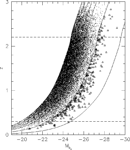
Figure 25: The redshift-absolute magnitude distribution of 2QZ (small points) and 6QZ (triangles) QSOs used in our analysis. The solid lines denote the apparent magnitude limits applied to the data, while the dashed lines show the redshift range used. A WMAP/2dF cosmology is assumed.

6.1 QSO clustering as a function of $b_{\rm J}$

We split the 2QZ QSOs into five sub-samples, on the basis of their apparent magnitude, $b_{\rm J}$. These intervals are listed in Table LABEL:tab:fitparmag. To enhance the dynamic range of this analysis we also include QSOs from the 6dF QSO Redshift Survey (6QZ; Paper XII). This data set contains 275 QSOs at $0.3<z<2.2$ in the magnitude range $16.0<b_{\rm J}<18.25$ selected from the same photometric data as the 2QZ. It forms a bright extension to the 2QZ, in the SGP region only (see Paper XII). All the QSOs in the 6QZ form a sixth magnitude interval. The distribution of QSOs in the $z-M_{\rm b_{\rm J}}$ plane is shown in Fig. 25. Even with the large sample presented here, the steep bright-end slope of the QSO luminosity function means that we can only cover an effective dynamic range of $\simeq 3$ mag in apparent magnitude (or a factor of $\simeq 16$ in luminosity). There is also only a relatively small dynamic range in QSO space density, from a mean $4.5\times 10^{-6}h^{3}{\rm Mpc}^{-3}{\rm mag}^{-1}$ at the faintest magnitudes to $9.2\times 10^{-7}h^{3}{\rm Mpc}^{-3}{\rm mag}^{-1}$. The greatest luminosity dependence might be expected for the brightest QSOs, as these are the rarest sources. This is exactly the point at which the rarity of QSOs makes clustering measurements most difficult. One solution to this problem is to cross-correlate QSOs of a given luminosity with QSOs at all other luminosities. This approach will be discussed by Loaring et al. (in preparation).

The measured $b_{\rm J}$ dependent $\xi(s)$ are shown in Fig. 26. At bright magnitudes (Fig. 26a) the small number and low space density of QSOs means that no significant signal is detected. At fainter magnitudes the data appear reasonably consistent with the best fit power law for the full sample (dotted lines). We also fit power laws to each $b_{\rm J}$ interval, showing the results as the solid lines in Fig. 26. The values are also listed in Table LABEL:tab:fitparmag. The best fit parameters vary considerably, but have large errors. Neither the slopes or amplitudes are particularly well constrained. If instead we fix $\gamma=1.2$ as found above, we find values of $s_{0}$ that are much closer to the mean (dashed lines in Fig. 26). We also note that the faintest magnitude interval (Fig. 26f) shows more structure on large scales than the other samples. It is possible that this is the result of increased incompleteness at the faint limit of the sample, even though we have taken care to correct for magnitude dependent spectroscopic completeness, as described in Paper XII. Estimation of $\xi(s)$ using the RA-Dec and RA-Dec-z mixing methods described above cause some reduction in this excess at large scales but does not completely remove it. This suggests that some, but not all, of this excess power could be due to residual incompleteness affects. Bearing this in mind we have checked whether any of our results above are affected by removing QSOs in the faintest bin from our sample and confirm that they have no significant impact on our conclusions.

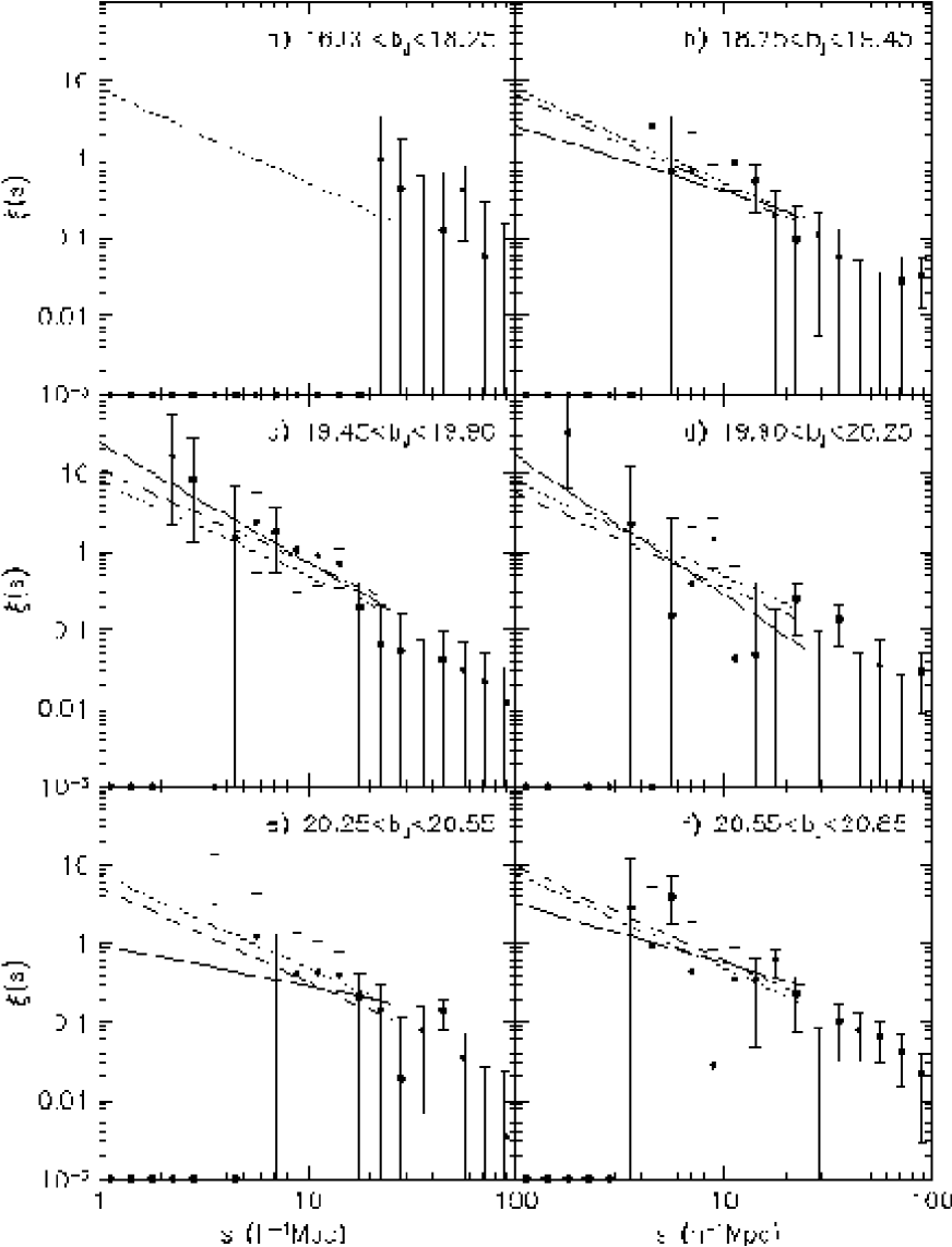
Figure 26: The QSO $\xi(s)$ from the 2QZ/6QZ (filled points) as a function of apparent $b_{\rm J}$ magnitude in 6 intervals from bright (a) to faint (f) magnitudes. The best fit power law is shown in each case (solid line) as is the best fit power law for the full sample for comparison (dotted line). We also show the best fit power law when fixing $\gamma$ to a value of 1.20 (dashed lines). No power law fit is attempted for the 6QZ data (a). A WMAP/2dF cosmology is assumed.

In order to use a robust measure of any luminosity dependence we calculate $\bar{\xi}(s)$ in each of the $b_{\rm J}$ intervals (Table LABEL:tab:fitparmag), which is plotted in Fig. 27. We confirm that the estimates of $\bar{\xi}$ are not significantly changed by using the RA-Dec mixing method to measure $\xi(s)$. We find that there is no significant evidence for any dependence of clustering amplitude with $b_{\rm J}$ (or equivalently luminosity relative to $L_{\rm Q}^{*}$). However, given the relatively large errors found [$\sim 30$ per cent in $\bar{\xi}(20)$] this result does not rule out models for which QSO clustering should be dependent on luminosity. As pointed out above, the mean space density of our brightest and faintest samples only differs by a factor of $\sim 5$. If this decrease in space density was solely due to higher mass (and therefore rarer) halos acting as hosts then this would correspond to a factor of $\sim 2$ increase in $M_{\rm DH}$, but only a $\sim 15$ per cent increase in bias (or $\sim 30$ per cent in clustering amplitude) which is approximately at the level of our measurement errors. This suggests that the increase in sensitivity provided by cross-correlating different QSO samples may provide useful constraints on QSO models (see Loaring et al. in preparation).

Figure 27: The dependence of $\bar{\xi}(s)$ on $b_{\rm J}$ for three different values of $s=20$, 30 and $50~{}h^{-1}~{}{\rm Mpc}$ (open circles, filled circles and open squares respectively). We do not plot a point at $s=20$, for the brightest bin, as there are no QSO pairs found.

7 conclusions

We have performed a detailed analysis of the clustering of 2QZ QSOs in redshift space as described by the two-point correlation function. Here we now discuss our conclusions.

The QSO two-point correlation function, $\xi(s)$, averaged over the redshift range $0.3<z<2.2$, shows a slope which changes as a function of scale, being flatter on small scales and steeper on large scales. A power law is an acceptable fit on scales less than $25~{}h^{-1}~{}{\rm Mpc}$ in a WMAP/2dF cosmology, the best fit parameters are $s_{0}=5.48_{-0.48}^{+0.42}~{}h^{-1}~{}{\rm Mpc}$ and $\gamma=1.20_{-0.10}^{+0.10}$. We demonstrate that QSO clustering on scales $<10~{}h^{-1}~{}{\rm Mpc}$ is strongly affected by non-linear $z$-space distortions, caused by redshift errors, shifts in QSO broad emission lines and intrinsic peculiar velocities, which all contribute similar amounts to the total velocity dispersion, of $\langle w_{\rm z}^{2}\rangle^{1/2}\simeq 690{\rm~{}km~{}s}^{-1}$. A power law model which has been corrected for both linear and non-linear $z$-space distortions is shown to be a good description of the shape of $\xi(s)$. Here we note that in modelling non-linear $z$-space distortions at high redshift it is important to include an extra factor of $1+z$ in Eq. 11 relative to the version normally used.

On large scales power law clustering is not an appropriate model and we therefore compare the 2QZ $\xi(s)$ to a model CDM $\xi(s)$ in a WMAP/2dF cosmology ($\Omega_{\rm m}=0.27$, $\Omega_{\Lambda}=0.73$, $\sigma_{8}=0.84$) accounting for the affects of non-linear clustering on small scales and the affects of $z$-space distortions. This model is well matched to the data after allowing for a linear bias of $b_{\rm Q}=2.02\pm 0.07$ at the mean redshift of the sample ($\bar{z}=1.35$). The 2QZ $\xi(s)$ also agrees remarkably well with that measured from the low redshift galaxies in the 2dFGRS [Hawkins et al. 2003], in both shape and amplitude. While the match in shape is unsurprising given that the physics (at least on large scales) prescribing the shape should be identical, the match in amplitude is impressive. Given that 2dFGRS galaxies are unbiased tracers of the mass distribution at low redshift [Verdi et al. 2002], it appears that the bias of QSOs exactly cancels out the growth of density fluctuations, to give a measured clustering equivalent to an unbiased population at low redshift. As we find evidence for evolution of QSO clustering in a WMAP/2dF cosmology, this agreement must be something of a coincidence. Also, in an EdS Universe the 2QZ $\xi(s)$ is a factor $\sim 2$ below the observed 2dFGRS clustering.

To further investigate these issues, we determine the clustering of 2QZ QSOs as a function of redshift. In a WMAP/2dF cosmology we find a significant (at the 98 per cent level) correlation of clustering amplitude with redshift as measured by the integrated correlation function within $20~{}h^{-1}~{}{\rm Mpc}$, $\bar{\xi}(20)$. Clustering increases with redshift and we find $\bar{\xi}(20)=0.263\pm 0.075$ at $z=0.53$, and $\bar{\xi}(20)=0.701\pm 0.174$ at $z=2.48$. In an EdS cosmology we find no evidence for evolution. By assuming an underlying WMAP/2dF cosmology we are able to directly determine the bias of QSOs, which we find to be a strong function of redshift. Even if there were no evolution in the measured $\bar{\xi}(20)$ with redshift, this would still imply a strongly evolving QSO bias. At low redshift, 2QZ QSOs appear largely unbiased, with $b_{\rm Q}(z=0.53)=1.13\pm 0.18$, while at high redshift we find $b_{\rm Q}(z=2.48)=4.24\pm 0.53$. A complication is that as the 2QZ is a flux limited sample, we are sampling more luminous QSOs at high redshift. However, the strong evolution of the QSO population means that to good approximation we are sampling the QSO population at the same space density at each redshift, and at the same point relative to the evolving break in the luminosity function, $L_{\rm Q}^{*}$. It thus appears that $L_{\rm Q}^{*}$ QSOs at low redshift should be largely unbiased, and clustered similarly to low redshift galaxies. This has indeed been seen by Croom et al. (2004) who cross-correlate low redshift (and therefore low luminosity) 2QZ QSOs with 2dFGRS galaxies and find no difference in the clustering properties of the two populations [see also Wake et al. (2004)].

By using the theoretical relation between $M_{\rm DH}$ and bias derived by Sheth et al. (2001) and others, it is possible for us to take the measured bias values for 2QZ QSOs and calculate the typical masses of their hosts’ DMHs. We find that the mass of DMHs hosting 2QZ QSOs is approximately constant with redshift, with a mean $M_{\rm DH}=(3.0\pm 1.6)\times 10^{12}h^{-1}M_{\odot}$. The fact that the hosts of 2QZ QSOs have the same mass at all redshifts demonstrates that they cannot be cosmologically long lived, as DMHs tend to grow and accumulate mass over time. Based on the formalism of Lacey & Cole (1993) we predict that DMHs hosting QSOs at $z\sim 2.5$ would typically have merged into DMHs of mass $\simeq 6\times 10^{14}h^{-1}M_{\odot}$ by the present, and therefore exist in rich galaxy clusters (although they would not generally be active at low redshift). In contrast, the descendents of lower redshift 2QZ QSOs would not have had time to form more massive halos, and should exist in either massive galaxies or groups. By extrapolation it is suggested that at $z=0$, $\sim L_{\rm Q}^{*}$ QSOs should also sit in $M_{\rm DH}=(3.0\pm 1.6)\times 10^{12}h^{-1}M_{\odot}$ halos, which is very close to the characteristic mass of the Press-Schechter mass function, $M^{*}(z=0)\simeq 3.5\times 10^{12}h^{-1}M_{\odot}$. The predicted growth of DMH mass by accretion/merging allows us to place upper limits on the lifetime of the QSO population. Low redshift QSOs cannot be the same population of objects as at higher redshift if they have masses which are less then the mass of the high redshift sources, after accounting for their expected growth over time. Therefore calculating the time taken to reach the mean QSO host DMH mass plus twice the measured rms gives a $\sim 2\sigma$ limit on the lifetime of QSO activity. We find this limit to be $t_{\rm Q}<6\times 10^{8}$ years at $z=2.48$, but weaker at low redshift ($3\times 10^{9}$ years at $z=0.53$). We note that this limit is not based on the measured number density of QSOs compared to a Press-Schechter mass function (as many other estimates are), but is only constrained by the clustering evolution of QSOs. Various authors have provided more detailed models in order to constrain the lifetime of QSO activity. When applied to our data, the model of Martini & Weinberg (2001) suggests that $z\sim 2$ QSOs will have lifetimes $t_{\rm Q}\simeq 4-50\times 10^{6}$ years. If there is scatter in the relation between $M_{\rm DH}$ and luminosity, then this is an effective lower limit on QSO lifetimes. The e-folding time for the evolution of $L^{*}_{\rm Q}$ is $\sim 2\times 10^{9}$ years (Paper XII), much less than the ages determined from the Martini & Weinberg model, and significantly less than our clustering evolution upper limits at high redshift.

As a next step we determine the central BH mass, $M_{\rm BH}$, of 2QZ QSOs based on their estimated $M_{\rm DH}$. For this we use the relations suggested by Ferrarese (2002) to estimate $M_{\rm BH}$ for different assumptions concerning the density profiles of the DMHs, and the evolution of the correlation [Wyithe & Loeb 2004]. A model in which the correlation between $M_{\rm BH}$ and $M_{\rm DH}$ is unchanging with redshift predicts that BH masses should be slightly increasing with redshift, with $\Delta\log(M_{\rm BH})\simeq 1.3\pm 1.1$ from the lowest to highest redshift. The derived BH masses are in the range $1-20\times 10^{7}M_{\odot}$ for NFW profiles, or $0.9-20\times 10^{8}M_{\odot}$ for S02 profiles. The Eddington ratio, $L/L_{\rm Edd}$, is seen to be approximately constant as a function of redshift when the $M_{\rm BH}-M_{\rm DH}$ relation is independent of redshift. This is found to be significantly greater than 1 if isothermal DMHs are assumed, and approximately 1 for the NFW profile, while the S02 profile gives $L/L_{\rm Edd}\sim 0.1$. A model in which it is the $M_{\rm BH}-\sigma_{\rm c}$ relation which is invariant with redshift gives a much stronger evolution of $M_{\rm BH}$ as DMHs of a given mass have a higher central velocity dispersion when formed at higher redshift. Thus the change in $M_{\rm BH}$ from low to high redshift is more significant with $\Delta\log(M_{\rm BH})\simeq 2.1\pm 1.1$, and BHs of order $\sim 10^{10}M_{\odot}$ being predicted at high redshift. This increase in estimated $M_{\rm BH}$ is greater than (although not significantly) the factor $\sim 30$ increase in mean luminosity from our lowest to highest redshift interval. As a result there is a small (factor of a few) decline in $L/L_{\rm Edd}$ with increasing redshift, although again this is not significant. As the BH masses predicted are higher, the accretion efficiencies are lower, in the range $L/L_{\rm Edd}\sim 0.01-1$ depending on DMH profile assumed.

The above suggests that any model of BH formation in which super-massive BHs form at least as efficiently at high redshift as they do at low redshift, will tend to have $L/L_{\rm Edd}$ constant or decreasing with redshift. This implies that it cannot be a reduction in efficiency which is driving the fading of the QSO population to low redshift. Instead active BHs at high redshift are more massive that those at low redshift, and it is this reduction in the BH mass that causes the population of bright QSOs to disappear in the local universe. Because super-massive BHs cannot be destroyed, the massive BHs active at high redshift must be largely inactive at low redshift, otherwise we would find that low redshift QSOs would show lower accretion efficiency, and be located in more massive DMHs. This argument also implies that at any given redshift, the QSO population must be dominated by objects which are active for the first time. Hence it is likely that each QSO passes through only one bright active epoch (possible at the point of BH formation), although at low redshift massive BHs may accrete at levels well below $L_{\rm Edd}$ without contributing significantly to the total luminosity of the population [see also the discussions in Corbett et al. (2003) and Croom et al. (2004b)].

The above is valid at redshift below $z\sim 2.5$, which is approximately the point at which the space density of luminous QSOs peaks. Clustering measurements of QSOs at $z>2.5$ would help us to understand the build up of QSOs at this epoch. However the low surface density of $z>2.5$ QSOs currently makes any accurate clustering measurements difficult or impossible. The increasing number of high redshift QSOs from the SDSS survey [Fan et al. 2001] may remedy this situation.

Finally, we examine our sample to look for any indication of luminosity dependence in the clustering of 2QZ QSOs, by measuring $\xi(s)$ as a function of apparent magnitude. This shows no indication of any luminosity dependence that might be expected if more luminous QSOs inhabited more massive DMHs, but the errors are large enough that we would not be able to detect reasonable amounts of luminosity dependence. More detailed investigation of this problem will be presented by Loaring et al. (in preparation).

References

- [Adelberger et al. 1998] Adelberger K.L., Steidel C.C., Giavalisco M., Dickinson M., Pettini M., Kellogg M., 1998, ApJ, 505, 18
- [Adelberger et al. 2003] Adelberger K.L., Steidel C.C., Shapley A.E., Pettini M. 2003, ApJ, 584, 45
- [Andreani & Cristiani 1992] Andreani P., Cristiani S., 1992, ApJ, 398, L13
- [Bahcall et al. 2003] Bahcall N.A., Dong F., Hao L., Bode P., Annis J., Gunn J.E., Schneider D.P., 2003, ApJ, 559, 814
- [Carroll et al. 1992] Carroll S.M., Press W.H., Turner E.L., 1992, ARA&A, 30 , 499
- [Condon et al. 1998] Condon J.J., Cotton W.D., Greisen E.W., Yin Q. F., Perley R.A., Taylor G.B., Broderick J.J., 1998, AJ, 115, 1693
- [Cole et al. 1998] Cole S.M., Hatton S., Weinberg D.H., Frenk C.S., 1998, MNRAS, 300, 945
- [Corbett et al. 2003] Corbett E.A. et al., 2003, MNRAS, 343, 705
- [Cristiani & Vio 1990] Cristiani S., Vio R., 1990, A&A, 227, 385
- [Croom et al. 2004a] Croom S.M., Smith R.J., Boyle B.J., Shanks T., Miller L., Outram, P.J., Loaring N.S., 2004a, MNRAS, 349, 1397 (Paper XII)
- [Croom et al. 2004b] Croom S.M., Schade D., Boyle B.J., Shanks T., Miller L., Smith R.J., 2004b, ApJ, 606, 126
- [Croom et al. 2004c] Croom S.M., et al. 2004c, in Richards G.T., Hall P.B., eds., ASP Conf. Ser. Vol. 311, AGN Physics with the Sloan Digital Sky Survey. Astron. Soc. Pac., San Francisco, p. 457 (astro-ph/0310533)
- [Croom et al. 2002] Croom S.M., Boyle B. J., Loaring N.S., Miller L., Outram, P.J., Shanks T., Smith R.J., 2002, MNRAS, 335, 459
- [Croom et al. 2001a] Croom S. M., Shanks T., Boyle B. J., Smith R. J., Miller L., Loaring N. S., Hoyle F., 2001a, MNRAS, 325, 483
- [Croom et al. 2001b] Croom S. M., Smith R. J., Boyle B. J., Shanks T., Loaring N. S., Miller L., Lewis I. J., 2001b, MNRAS, 322, L29
- [Croom & Shanks 1996] Croom S.M., Shanks T., 1996, MNRAS, 281, 893
- [Evrard et al. 2002] Evrard, A.E. et al. 2002, ApJ, 573, 7
- [Fan et al. 2001] Fan X. et al., 2001, AJ, 122, 2833
- [Ferrarese & Merritt 2000] Ferrarese, L. & Merritt, D., ApJ, 539, L9
- [Ferrarese 2002] Ferrarese L., 2002, ApJ, 578, 90
- [Frenk et al. 2000] Frenk C .S. et al. 2000, astro-ph/0007362
- [Foucaud et al. 2003] Foucaud S. et al., 2003, A&A, 409, 835
- [Fry 1996] Fry N.J., 1996, ApJ, 461, L65
- [Grazian et al. 2004] Grazian A. et al., 2004, AJ, 127, 592
- [Gebhardt et al.2000] Gebhardt, K., et al. 2000, ApJ, 539, L13
- [Gehrels 1986] Gehrels N., 1986, ApJ, 303, 336
- [Haiman & Hui 2001] Haiman Z., Hui L., 2001, ApJ, 547, 27
- [Hamilton et al. 1991] Hamilton A.J.S., Kumar P., Lu E., Matthews A., 1991, ApJ, 374, L1
- [Hamilton et al. 1995] Hamilton A.J.S., Kumar P., Lu E., Matthews A., 1995, ApJ, 442, L73
- [Hamilton 1992] Hamilton A. J. S., 1992, ApJ, 385, L5
- [Hawkins et al. 2003] Hawkins E. et al., 2003, MNRAS, 346, 78
- [Hoyle 2000] Hoyle F., 2000, Ph.D. Thesis, University of Durham
- [Hoyle et al. 2002] Hoyle F., Outram P. J., Shanks T., Boyle B. J., Croom S. M., Smith R. J., 2002, MNRAS, 332, 311
- [Iovino & Shaver 1988] Iovino A., Shaver P.A., 1988, ApJ, 330, L13
- [Jain et al. 1995] Jain B., Mo H.J., White S.D.M., 1995, MNRAS, 276, L25
- [Jing 1998] Jing Y.P., 1998, ApJ, 503, L9
- [Kaiser 1987] Kaiser N., 1987, MNRAS, 227, 1
- [Kaspi et al. 2000] Kaspi S., Smith P. S., Netzer, H., Maoz, D., Januzzi, B. T., Giveon, U., 2000, ApJ, 533, 631
- [Kauffmann & Haehnelt 2002] Kauffmann G., Haehnelt M.G., 2002, MNRAS, 332, 529
- [Kukula et al. 2001] Kukula M. J., Dunlop J. S., McLure R. J., Miller L., Percival W. J., Baum S. A., O’Dea C. P. 2001, MNRAS, 326, 1533
- [Lacey & Cole 1993] Lacey C., Cole S., 1993, MNRAS, 262, 627
- [La Franca et al. 1998] La Franca F., Andreani P., Cristiani, S., 1998, ApJ, 497, 529
- [Landy & Szalay 1993] Landy, S.D., Szalay, A.S., 1993, ApJ, 412, 64
- [Matsubara & Suto 1996] Matsubara T., Suto Y., 1996, ApJ, 470, L1
- [Martini & Weinberg 2001] Martini P., Weinberg D.H., 2001, ApJ, 547, 12
- [McLure & Dunlop 2004] McLure R.J., Dunlop J.S., 2004, MNRAS, 352, 1390
- [Miller et al. 2003] Miller C.J., Nichol R.C., Gómez P.L., Hopkins A.M., Bernardi M., 2003, ApJ, 597, 142.
- [Miller et al 2004] Miller L., Croom S.M., Boyle B.J., Loaring N.S., Smith R.J., Shanks T., Outram P.J., 2004, MNRAS submitted (astro-ph/0403065)
- [Mo & Fang 1993] Mo H.J., Fang L.Z., 1993, ApJ, 410, 493
- [Mo & White 1996] Mo H.J., White S.D.M., 1996, MNRAS, 282, 347
- [Navarro et al. 1997] Navarro J.F., Frenk C.S., White S.D.M., 1997, ApJ, 490, 493 (NFW)
- [Norberg et al. 2001] Norberg P. et al., 2001, MNRAS, 328, 64
- [Osmer 1981] Osmer P.S., 1981, ApJ, 247, 762
- [Outram et al. 2004] Outram P.J. et al., 2004, MNRAS, 348, 745
- [Outram et al. 2003] Outram P.J. et al., 2003, MNRAS, 342, 483
- [Overzier et al. 2003] Overzier R.A., Röttgering H.J.A., Rengelink R.B., Wilman R.J., 2003, A&A, 405, 53
- [Percival et al. 2002] Percival W., et al., 2002, MNRAS, 337, 1068
- [Postman et al. 1998] Postman M., Lauer T.R., Szapudi I., Oegerle W., 1998, ApJ, 506 33
- [Press & Schechter 1974] Press W.H., Schechter P., 1974, ApJ, 187, 425
- [Ratcliffe et al. 1998] Ratcliffe A., Shanks T., Parker Q.A., Fong R., 1998, MNRAS, 296, 191
- [Richards et al. 2002] Richards G.T. et al. 2002, AJ, 124, 1
- [Roukema et al 2002] Roukema B. F., Mamon G. A., Bajtlik, S., 2002, A&A, 382, 397
- [Schade et al 2000] Schade D., Boyle B.J., Letawsky M., 2000, MNRAS, 315, 498
- [Schlegel et al. 1998] Schlegel D.J., Finkbeiner D.P., Davis M., 1998, ApJ, 500, 525
- [Seljak 2002] Seljak U., 2002, MNRAS, 334, 797 (S02)
- [Shanks et al. 1987] Shanks T., Fong R., Boyle B.J., Peterson B.A., 1987, MNRAS, 227, 739
- [Shanks & Boyle 1994] Shanks T., Boyle B.J., 1994, MNRAS, 271, 753
- [Shaver 1984] Shaver P.A., 1984, A&A, 136, L9
- [Sheth et al. 2001] Sheth R.K., Mo H.J., Tormen G., 2001, MNRAS, 323, 1
- [Shields et al. 2003] Shields G.A., Gebhardt K., Salviander S., Wills B.J., Xie B., Brotherton M.S., Yuan J., Dietrich M., 2003, ApJ, 583, 124
- [Steidel et al. 1998] Steidel C.C., Adelberger K.L., Dickinson M., Giavalisco M., Pettini M., Kellogg M., 1998, ApJ, 492, 428
- [Spergel et al. 2003] Spergel D. N., et al., 2003, ApJS, 148, 175
- [Ueda et al. 2003] Ueda Y., Akiyama M., Ohta K., Miyaji T., 2003, ApJ, 598, 886
- [Verdi et al. 2002] Verdi L. et al., 2002, MNRAS, 335, 432
- [Wake et al. 2004] Wake D.A. et al., 2004, ApJ, 610, L85
- [Wyithe & Loeb 2004] Wyithe J.S.B., Loeb A., 2004, ApJ submitted (astro-ph/0403714)