The DEEP2 Galaxy Redshift Survey: Probing the Evolution of Dark Matter Halos around Isolated Galaxies from $z\sim 1$ to $z\sim 0$

Abstract

Using the first 25% of DEEP2 Redshift Survey data, we probe the line-of-sight velocity dispersion profile for isolated galaxies with absolute B-band magnitude $-22<M_{B}-5\log(h)<-21$ at $z$=0.7-1.0, using satellite galaxies as luminous tracers of the underlying velocity distribution. Measuring the velocity dispersion beyond a galactocentric radius of $\sim 200h^{-1}$kpc (physical) permits us to determine the total mass, including dark matter, around these bright galaxies. Tests with mock catalogs based on N-body simulations indicate that this mass measurement method is robust to selection effects. We find a line-of-sight velocity dispersion ($\sigma_{los}$) of $162^{+44}_{-30}$ km s^-1 at $\sim 110h^{-1}$ kpc, $136^{+26}_{-20}$ km s^-1 at $\sim 230h^{-1}$ kpc, and $150^{+55}_{-38}$ km s^-1 at $\sim 320h^{-1}$ kpc. Assuming an NFW model for the dark matter density profile, this corresponds to a mass within r₂₀₀ of $M_{200}=5.5^{+2.5}_{-2.0}\times 10^{12}h^{-1}$M_☉ for our sample of satellite hosts with mean luminosity $\sim 2.5L^{\ast}$. Roughly $\sim 60\%$ of these host galaxies have early-type spectra and are red in restframe $(U-B)$ color, consistent with the overall DEEP2 sample in the same luminosity and redshift range. The halo mass determined for DEEP2 host galaxies is consistent with that measured in the Sloan Digital Sky Survey for host galaxies within a similar luminosity range relative to $M^{\ast}_{B}$. This comparison is insensitive to the assumed halo mass profile, and implies an increase in the dynamical mass-to-light ratio ($M_{200}/L_{B}$) of isolated galaxies which host satellites by a factor of $\sim 2.5$ from $z\sim 1$ to $z\sim 0$. Our results can be used to constrain the halo occupation distribution and the conditional luminosity function used to populate dark matter halos with galaxies. In particular, our results are consistent with scenarios in which galaxies populate dark matter halos similarly from $z\sim 0$ to $z\sim 1$, except for $\sim 1$ magnitude of evolution in the luminosity of all galaxies. With the full DEEP2 sample, it will be possible to extend this analysis to multiple luminosity or color bins.

1. Introduction

It has been firmly established that galaxies and clusters form within halos whose mass is dominated by unseen dark matter. Yet until very recently, the outer regions of halos have been very poorly understood due to a lack of visible tracers of the mass distribution. Galaxy-galaxy lensing is able to probe the halo masses of local galaxies, though with some degree of uncertainty, as this method actually probes all of the mass along the line-of-sight (Guzik & Seljak 2002), and has only recently been applied to isolated galaxies (Hoekstra et al. 2005). Recent work (Wilson et al. 2001; Hoekstra, Yee, & Gladders 2004; Kleinheinrich et al. 2005) suggests that the virial mass of $\sim L^{\ast}$ galaxies has remained constant from $z\sim 0.8$ to $z\sim 0.15$. Beyond $z\sim 0.5$ the lensing probability rapidly diminishes, making it very difficult to derive masses of isolated galaxies (with masses $\sim 10^{12}M_{\sun}$) with this method at higher redshift (see e.g., Peacock 1999).

The dynamics of satellite galaxies orbiting larger “host” galaxies provide another way to probe the mass distribution at large radii. Early work by Little & Tremaine (1987); Erickson, Gottesman, & Hunter (1987); Zaritsky et al. (1989) utilized samples of tens of satellites as early confirmation that galaxies are embedded in large dark matter halos. More conclusive evidence was compiled by Zaritsky et al. (1993, 1997) who used the kinematics of a sample of 115 satellite galaxies to probe the outer regions of 69 isolated galaxies. By employing satellites as test particles, they built up a velocity profile for a single representative isolated galaxy by stacking measurements of satellites from many different host galaxies.

More recently, Prada et al. (2003, hereafter P03) use $\sim$250,000 SDSS redshifts to probe the halo masses of isolated galaxies; they detect $>$1000 satellites around $\sim$700 host galaxies. With this large data set they are able to discriminate between various halo mass distributions and find evidence for an NFW-like falloff ($\rho\propto r^{-3}$) at large radii. From these accurate line-of-sight velocity dispersion profile measurements, P03 infer the masses enclosed within 1.5 R_virial for two sets of isolated galaxies. Host galaxies with $-20.5<M_{B}<-19.5$ are found to have an average halo mass of $M_{virial}\approx 1.5\times 10^{12}M_{\sun}$ while hosts with $-21.5<M_{B}<-20.5$ have $M_{virial}\approx 6\times 10^{12}M_{\sun}$ (for $h=0.7$). Other recent work utilizing satellite dynamics includes McKay et al. (2002), who check SDSS weak-lensing scaling laws; van den Bosch et al. (2004a, b), who use mock galaxy catalogs and the 2dF survey to constrain the conditional luminosity function and investigate the levels and effects of contamination in dynamical satellite studies; and Brainerd (2005), who measure velocity dispersion profiles for subsamples of isolated 2dF galaxies.

By extending this type of measurement to high redshift, we can study the evolution of the relationship between galaxies and dark matter halos. There have been few ways to do this until the recent advent of large, high-redshift surveys. The best example to date is Yan, Madgwick, & White (2003), who use the 2dF and DEEP2 two-point correlation functions (Madgwick et al. 2003a; Coil et al. 2004, respectively) to constrain the evolution of the halo occupation distribution, a key ingredient of the halo model. Yan et al. produced a set of $z\sim 1$ mock catalogs using N-body simulations and a halo model whose parameters are set by requiring a fit to $\xi(r)$ from 2dF at $z\sim 0$. They find good agreement between the correlation statistics at $z\sim 0.8$ from DEEP2 and the prediction from these mock catalogs, which populate galaxies in dark matter halos in the same way (as a function of $L/L^{\ast}$ and halo mass) at $z\sim 1$ and $z\sim 0$. Hence their results are consistent with a minimal-evolution hypothesis, in which galaxies with a given luminosity compared to $L^{\ast}$ at $z\sim 1$ live in the same sorts of halos as similar galaxies at $z\sim 0$, though the mass function of dark matter halos and $L^{\ast}$ evolve. Here we address this hypothesis with an independent method.

In this paper we constrain the velocity dispersion profile for a typical isolated DEEP2 galaxy at $z\sim 0.8$ using methods similar to those of P03. We then deduce a representative halo mass for these galaxies and compare our results to recent local measurements from SDSS to test for evolution in a self-consistent way. We use mock catalogs to test the significance and robustness of these results. The paper proceeds as follows. In $\S$ 2 we describe the DEEP2 data set and the properties of satellite galaxies and their hosts. $\S$ 3 outlines our method for reconstructing the mass of isolated galaxies using satellites and in $\S$ 4 we present our results and compare with recent local measurements. We test our methods using mock catalogs in $\S$ 5 and discuss some implications of our results in $\S$ 6. Throughout the paper we assume a standard $\Lambda$CDM cosmology with $\Omega_{m}=0.3$, $\Omega_{\Lambda}=0.7$ and H${}_{0}=100h^{-1}$ km s^-1 Mpc^-1. Absolute magnitudes quoted have been K-corrected and corrected for reddening by galactic dust, and are in the AB system (Willmer et al. 2005).

2. Satellite-Host Systems at $z\sim 1$

In this Section we introduce the data used at $z\sim 1$, describe the algorithm used to identify bright isolated galaxies and their satellites, and highlight several properties of these host-satellite systems.

We use data from the first $\sim 25\%$ of the DEEP2 Galaxy Redshift Survey, a three-year project using the DEIMOS spectrograph at the 10-m Keck II telescope to survey galaxies at $z\sim 1$. DEEP2 will collect spectra of $\sim$50,000 galaxies from $0.7<z<1.4$ to a limiting magnitude of $R_{AB}=24.1$ with redshift errors of $\sim$20 km s^-1. For survey details, see Davis et al. (2004). Photometric data were taken in the $B,R$ and $I$ bands with the CFH12k camera on the 3.6-m Canada-France-Hawaii telescope. We use data taken during the first two seasons of DEEP2 observations, which have yielded $\sim$12,000 secure redshifts over $\sim$0.9 sq. degrees. Our observed R-band limiting magnitude corresponds to a different restframe wavelength with redshift, from $4000\AA$ at $z=0.7$ to $2800\AA$ at $z=1.4$. This results in a different selection function for red and blue galaxies with redshift, such that as we move to fainter magnitudes, red galaxies become undetectable before blue galaxies; this effect increases with increasing redshift (see Willmer et al. 2005, for details). To minimize this effect we consider only bright hosts with $z<1$.

We define an isolated galaxy as having no bright neighbors within a given search cylinder. Once isolated galaxies have been identified, we use another search cylinder to identify faint satellite companions. Specifically, a galaxy is isolated if it has no neighbors in the DEEP2 spectroscopic sample within a physical distance projected on the sky $r_{p}<350h^{-1}$kpc, line-of-sight velocity difference $|\Delta v|<1000$ km s^-1 and absolute magnitude difference $\Delta M_{B}<1.5$. An isolated galaxy furthermore cannot have any neighbors within $350h^{-1}$kpc$<r_{p}<700h^{-1}$kpc and $|\Delta v|<1000$ km s^-1 with $\Delta M_{B}<0.75$; we relax our magnitude cut at large $r_{p}$ because galaxies this far apart will be less dynamically associated. Satellites are similarly defined to be galaxies with $r_{p}<350h^{-1}$ kpc, $|\delta v|<500$ km s^-1 and $\delta M_{B}>1.5$; i.e. satellites must be more than 1.5 magnitudes fainter than the host galaxy they belong to. These parameters define sample 1 in Table 1 which lists the search parameters used in this analysis along with the number of found satellites and several derived host halo parameters. We consider 7 different search criteria and find that the results presented are quite insensitive to variations in these criteria; for convenience we quote results from sample 1 unless otherwise noted. Our choices of parameters ensure that a satellite can be associated with one and only one host galaxy. We put no restriction on morphological or spectral type, but require the isolated host galaxy to have $-22<M_{B}-5\log(h)<-21$ and $0.7<z<1.0$.

Figure 1.— Characteristics of isolated host galaxies. Upper left: absolute B-band magnitude of hosts. Upper right: redshift distribtion. Lower left: first PCA eigenvalue for host galaxy spectra. The dashed line indicates the division between late types ($\eta>-13$) and early types ($\eta<-13$). Lower right: number of satellite galaxies found per host.

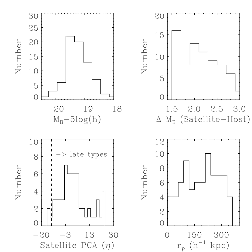
Figure 2.— Characteristics of satellite galaxy properties. Upper left: satellite galaxy absolute B-band magnitude. Upper right: $\Delta M_{B}$ between host and satellite. Lower left: satellite galaxy spectra type. The dashed line indicates the division between late and early type spectra. Lower right: projected separation (physical units) on the sky between satellite and host. Slit collisions reduce the number of satellites found with $r_{p}<50h^{-1}$ kpc.

For our chosen set of search parameters (Sample 1), we have identified 75 satellites around a total of 61 host galaxies at $0.7<z<1.0$ in the DEEP2 data set. Figures 1 and 2 show relevant characteristics of the satellite and host galaxies including distributions in redshift, spectral-type, absolute magnitude, satellite number per host, satellite distance from host, and $\Delta M_{B}$ between the host and satellite. We determine spectral types using the principal component analysis of Madgwick et al. (2003b) and use their definition of $\eta=-13$ to separate early and late-type galaxies. Galaxy morphology and $(U-B)_{0}$ color correlate well with this spectral classification of early and late types (Madgwick 2003)). Satellites are found to have $\sim 90\%$ late-type spectra, but due to the DEEP2 survey selection effects mentioned above, it is difficult to determine if this is an intrinsic property of satellites around bright isolated galaxies, or due to the $R$-band selection of the survey. As we observe fainter galaxies (e.g. satellites), early-type galaxies become undetectable before late-type galaxies.

Figure 3.— Color-Magnitude diagram for all isolated host galaxies from sample 1 (stars) compared to a subsample of the first two seasons of DEEP2 data (points). The subsample was constructed to have the same redshift distribution as the host galaxies, thus reducing any potential redshift dependent selection effects. Dashed lines indicate the magnitude range we have used in computing halo masses. We classify galaxies with $(U-B)_{0}>$1 “red” and $(U-B)_{0}<$1 “blue”.

We find that approximately 60% of host galaxies have early-type spectra. When we select a subsample of the entire available DEEP2 data set such that it has the same redshift and absolute magnitude distributions as the host galaxies, we find that both sets of objects have consistent fractions of early-type galaxies: 58% for isolated hosts and 63% for the subsample. This result is somewhat surprising; one might have naively suspected that the majority of early-type galaxies with $-22<M_{B}-5\log(h)<-21$ would reside in dense environments and hence would not be identified as isolated using our search criteria. To test the robustness of this result, we also use $(U-B)_{0}$ color to test for any differences between isolated galaxies and our reconstructed subsample. Again we find that $\sim 55\%$ of isolated host galaxies are red ($(U-B)_{0}>$1), while $\sim 50\%$ of the subsample is red (see Fig. 3). There thus seems to be a significant population of bright, red, early-type isolated galaxies with satellites at $z\sim 1$. Our host galaxies have approximately the same relative number of early and late spectral types as in P03’s sample; this will allow for robust comparisons between halo masses using SDSS data at $z\sim 0$ and DEEP2 data at $z\sim 1$.

3. Halo Mass Estimation

In this section we describe our method for obtaining dark matter halo masses for isolated galaxies utilizing satellite galaxy kinematics. Our approach is similar to previous work (see e.g. Prada et al. 2003; Brainerd & Specian 2003), except for our maximum-likelihood approach to deriving velocity dispersions which is more robust than previous methods when applied to small numbers of host-satellite pairs.

Schematically, we derive masses in the following way. First we obtain a sample of isolated galaxies with associated satellites. We then measure the line-of-sight velocity dispersion in several radial bins for a “typical” isolated bright galaxy, using satellites as luminous tracers of the velocity field. In our sample, each isolated galaxy has at most three or four satellites, but we can measure dispersions by stacking the satellite-host pairs and thereby treating all satellites as belonging to a single typical host galaxy. In implementing this method we are assuming that similarly bright isolated galaxies reside in similar halos. We create an homogeneous host galaxy sample by searching for satellites around galaxies with $-22<M_{B}-5\log(h)<-21$ and $0.7<z<1.0$. As more data becomes available, it will be possible to limit these criteria even further, yielding results for multiple luminosity, redshift, color, and spectral type bins.

In order to determine line-of-sight velocity dispersions, we build distributions of the projected velocity difference between satellite and host ($\delta v$) in bins of projected radius from the host galaxy and fit for the dispersion in the distribution. To convert the resulting velocity dispersion measurements into a mass, we make several assumptions, including the shape of the underlying dark matter potential. We now describe this procedure in detail.

3.1. Velocity Dispersion Measurement

The difference between the host and satellite galaxy line-of-sight velocity, $\delta v$, has a distribution that is well fit by a Gaussian of zero mean. In the absence of interlopers (see below), the satellite velocity dispersion, $\sigma_{los}$ can simply be obtained from the width of a Gaussian fit to the velocity distribution. In order to be able to detect variation in the velocity profile with radius, we bin the satellites in projected radius, $r_{p}$, from the host galaxy. We have chosen bins such that the number of satellites per bin is roughly constant: $30<r_{p}<180$, $180<r_{p}<280$, and $280<r_{p}<350$, in units of $h^{-1}$ kpc; these choices assure similar errors from bin to bin.

An important aspect of this analysis is the careful rejection of “interlopers”; these are galaxies which meet the criteria for satellite identification, but are in fact not dynamically associated with the host. Interlopers result from peculiar velocities which can, in redshift space, scatter objects into our search cylinder. Recent local studies (e.g. P03, van den Bosch et al. 2004a) have found that about 20-30% of putative satellites fall into this category.

Since interlopers are not physically associated with the host galaxy, we account for them by assuming that they will have a constant $\delta v$ distribution. Thus, we expect the observed $\delta v$ distribution be a combination of flat (interloper) and Gaussian (true satellite) components. We therefore fit a Gaussian plus constant distribution to the velocity measurements within each $r_{p}$ bin. If we ignore clustering effects, which is reasonable since we are only probing isolated systems, then one would expect the number density of interlopers to simply scale with the search volume. Although the interloper fraction should be roughly constant in $\delta v$, that constant should be different in bins of different radii. This is another important motivation for measuring $\sigma_{los}$ in bins of $r_{p}$.

Unlike previous studies which fit Gaussian profiles to velocity histograms, we determine the dispersion of the velocity distribution using a maximum likelihood Gaussian-plus-constant fit to the unbinned $\delta v$ data. Specifically, our likelihood function:

$$L(a,\sigma_{los},i)=a+Be^{-\delta v_{i}^{2}/(2\sigma_{los}^{2})},$$ (1)

has two free parameters, a constant component (in satellites per km/s), $a$, and the width of the Gaussian, $\sigma_{los}$. The parameter $B$ is chosen such that the integral of the probability density function of the relative velocity distribution between host and satellite (given $a$ and $\sigma_{los}$) over the allowed velocity range is one, and $\delta v_{i}$ is the $\delta v$ for the $i$th satellite-host pair. We maximize the summed logarithm of this likelihood function:

$$S(a,\sigma_{los})=\sum_{i}ln(L)$$ (2)

over a dense grid in $\sigma_{los}$ and $a$.

In Monte Carlo tests, this algorithm agrees with method of fitting Gaussian distributions to velocity histograms for well-sampled data, but is much more robust in the limit of small numbers of satellites. This technique also provides an estimate of the error in the velocity dispersion measurement from the width of the likelihood peak.

3.2. Halo Mass Determination

In order to derive a host halo mass, we fit a theoretical velocity dispersion profile to the measured velocity dispersion points. The theoretical profile is obtained via the following procedure. We start by assuming an NFW (Navarro, Frenk, & White 1996, 1997) density distribution

$$\frac{\rho(r)}{\rho^{0}_{c}}=\frac{\delta_{c}}{(r/r_{s})(1+r/r_{s})^{2}}$$ (3)

($\rho\propto r^{-3}$ for large r) where $\rho^{0}_{c}$ is the present critical density, $r_{s}=r_{200}/c$, and

$$\delta_{c}=\frac{200}{3}\frac{c^{3}}{ln(1+c)-c/(1+c)}$$ (4)

where $r_{200}$, defined as the radius where the mean interior density is 200 times the critical density. The concentration, $c$, can be viewed as a free parameter determining the shape of the NFW density profile. In general the concentration is inversely related to the mass of a dark matter halo.

The Jeans equation is then used to relate the radial velocity dispersion, $\sigma_{r}$, to the gravitational potential, $\Phi$,

$$\frac{1}{\rho}\frac{d}{dr}(\rho\sigma_{r}^{2})+2\beta\frac{\sigma_{r}^{2}}{r}=-\frac{d\Phi}{dr}$$ (5)

and then we integrate along the line of sight

$$\sigma_{los}^{2}(r_{p})=\frac{2}{\Sigma_{M}(r_{p})}\int_{r_{p}}^{\infty}(1-\beta\frac{r_{p}^{2}}{r^{2}})\frac{\rho\sigma_{r}^{2}(r,\beta)r}{\sqrt{r^{2}-r_{p}^{2}}}dr$$ (6)

where

$$\Sigma_{M}(r_{p})=2\int_{r_{p}}^{\infty}\frac{r\rho(r)}{\sqrt{r^{2}-r_{p}^{2}}}dr$$ (7)

is the surface mass density (see Łokas & Mamon (2001) for details of these calculations). In the above, $r$ is the radial distance and $r_{p}$ is, as usual, the distance projected on the sky. The velocity anisotropy ($\beta\equiv 1-\sigma_{r}^{2}/\sigma_{\perp}^{2}$, where $\sigma_{r}$ is the radial velocity dispersion and $\sigma_{\perp}$ is the velocity dispersion perpendicular to the line of sight) must be assumed in the conversion of the NFW density profile to a velocity dispersion profile; we use an Osipkov-Merrit anisotropy, $\beta_{OM}=s^{2}/(s^{2}+s_{a}^{2})$, with $s_{a}=4/3$ and $s=r/r_{200}$. van den Bosch et al. (2004a) and (Mamon & Łokas 2005) find that the line-of-sight velocity dispersion profile depends only weakly on $\beta$, at the level of a few percent, and hence we do not explore other parameterizations. We further need to assume the concentration; we use $c=10$, which is consistent with our fit to the mock catalog velocity dispersion profiles (see $\S$ 5), and is in general in agreement with simulations of $\sim 10^{12}M_{\sun}$ halos. In $\S$ 4 we show that our results concerning the evolution of the halo mass of isolated galaxies are insensitive to the assumed concentration. With these assumptions we are left with only one free parameter, the normalization of the velocity dispersion profile, which can be characterized by the circular velocity at $r_{200}$, $V_{200}$. We fit for $V_{200}$ via $\chi^{2}$ minimization using the observed data points. For the same enclosed region, the interior mass ($M_{200}$) can be easily inferred from $V_{200}$ for a given cosmology (see Navarro, Frenk, & White 1996, 1997, for details).

4. Results

Using the maximum likelihood method outlined in $\S$ 3, we measure a velocity dispersion of $162^{+44}_{-30}$ km s^-1 for satellites with $30<r_{p}<180h^{-1}$kpc (median $r_{p}=110h^{-1}$kpc), $136^{+26}_{-20}$ km s^-1 for $180<r_{p}<280h^{-1}$kpc (median $r_{p}=230h^{-1}$kpc), and $150^{+55}_{-38}$ km s^-1 for $280<r_{p}<350h^{-1}$kpc (median $r_{p}=320h^{-1}$kpc) for isolated galaxies with $-22<M_{B}-5\log(h)<-21$ (see Fig. 4). Errors on the velocity dispersion are derived from the maximum-likelihood fit. These results are robust to changes in the search parameters and radial binning; for the 7 different search criteria listed in Table 1, our line-of-sight velocity dispersion measurements vary within 1$\sigma$ of the dispersions quoted above. From Fig. 4 it is clear that the derived dispersion profile is consistent with nearly all popular halo mass density profiles (e.g. isothermal, NFW, Moore (Moore et al. 1998)), though we use an NFW profile to derive masses. What is important for this analysis is the normalization of the velocity dispersion profile, not the slope, as long as the slope at $V_{200}$ is shallow.

Figure 4.— Line-of-sight velocity dispersion profile for a typical isolated bright galaxy in the DEEP2 sample. The line with error bars is the profile derived from the DEEP2 sample; the dotted curve is a best fitting NFW line-of-sight velocity dispersion profile ($c=10$ assumed). The line with errors is very stable over a wide range of search parameters and variation in the radial binning. The individual points are the $\Delta v$ and $r_{p}$ of the satellite-host systems. The best fit NFW profile (dashed line) corresponds to a mass of $M_{200}=5.5\times 10^{12}h^{-1}M_{\sun}$.

As outlined in $\S$ 3, we fit velocity dispersion profiles derived from an NFW model to the measured velocity dispersion profile for DEEP2 by minimizing $\chi^{2}$. Our results imply a total mass, $M_{200}$, of $5.5^{+2.5}_{-2.0}\times 10^{12}h^{-1}M_{\sun}$ for a typical isolated galaxy with $-22<M_{B}-5\log(h)<-21$ and at least one satellite. When we vary the search criteria the measured mass varies by $\pm 1\times 10^{12}h^{-1}M_{\sun}$, within our 1$\sigma$ errors (see Table 1). As mentioned above, interlopers play a key role in this analysis. From our best fitting Gaussian plus constant fit to the satellite $\delta v$ distribution, we find that the interloper fraction increases with increasing $r_{p}$, from $\sim 7$% at $r_{p}\sim 110h^{-1}$ kpc to $\sim 30$% at $r_{p}=320h^{-1}$ kpc. These numbers are in good agreement with previous results from P03 and van den Bosch et al. (2004a).

We can compare this derived mass to recent local measurements to measure evolution in the halo mass of isolated galaxies. Unfortunately, we could not implement the exact same search criteria as in P03 as that yields only 30 satellites in the DEEP2 sample, too few to provide robust results. Thus, in order to make a fruitful comparison, we have taken the raw $\Delta v$ and $r_{p}$ measurements of P03 (F. Prada 2004, private communication) and independently determined the underlying halo mass using our own host galaxy magnitude range and search criteria. We note that our methods accurately recover the masses inferred in P03’s samples (see $\S$ 1) when using their definitions and absolute magnitude intervals.

Figure 5.— As Fig. 4, but for SDSS satellite galaxies from P03 (data provided by F. Prada). The best fitting NFW line-of-sight velocity dispersion profile implies an average halo mass $M_{200}$ of $5.4^{+1.2}_{-1.0}\times 10^{12}h^{-1}M_{\sun}$. The lack of points past $r_{p}=350h^{-1}$kpc is a result of the definition of satellites in the P03 dataset.

Taking $M^{*}_{B}(z\sim 0)-5\log(h)=-19.45\pm 0.07$ (Norberg et al. 2002, this value was converted from the $b_{j}$-band by assuming a median color of $B-V=0.21$) and $M^{*}_{B}(z\sim 1)-5\log(h)=-20.6\pm 0.1$ (Willmer et al. 2005), we use 475 host galaxies in the P03 sample with magnitudes $-21<M_{B}-5\log(h)<-20$ ensuring that the samples at $z\sim 1$ and $z\sim 0$ have similar host galaxy magnitude ranges relative to $M^{*}_{B}$. We find isolated galaxies at $z\sim 0$ with $-21<M_{B}-5\log(h)<-20$ to have an average halo mass of $5.4^{+1.2}_{-1.0}\times 10^{12}h^{-1}M_{\sun}$ when assuming an NFW mass density distribution with $c=10$ (see Fig. 5).

We can cast these results in terms of the dynamical mass to B-band light ratio, $M_{200}/L_{B}$. Using the mean luminosity of host galaxies at $z\sim 1$ of $M_{B}-5\log(h)=-21.5\pm 0.1$ ($L_{B}=5.3\pm 0.5\times 10^{10}h^{2}L_{\sun}$) and at $z\sim 0$ of $M_{B}-5\log(h)=-20.5\pm 0.1$ ($L_{B}=2.1\pm 0.1\times 10^{10}h^{2}L_{\sun}$), we find that the $B$-band mass-to-light ratio ($M_{200}/L_{B}$) is increasing from $M_{200}/L_{B}=104\pm 43$ $hM_{\sun}/L_{\sun,B}$ at $z\sim 1$ to $M_{200}/L_{B}=257\pm 54$ $hM_{\sun}/L_{\sun,B}$ at $z\sim 0$, a factor of 2.5. Total (random and systematic) errors in our absolute magnitude measurements, including uncertainties in K corrections apart from the assumed cosmological parameters, are estimated to be below $0.1$ mag at the redshifts of interest (Willmer et al. 2005); hence errors in luminosities are negligible compared to the statistical uncertainties in the average $M_{200}/L_{B}$.

5. Testing the Method

We use mock galaxy catalogs that have been constructed to match the DEEP2 survey in order to test whether we can accurately recover the halo mass of isolated galaxies using satellites. A complete description of the catalogs are given in Yan et al. (2004); we give the relevant details here. N-body simulations of $512^{3}$ dark matter particles with a particle mass $m_{part}=1.0\times 10^{10}$ h${}^{-1}M_{\sun}$ were run in a $\Lambda$CDM Universe using the TreePM code (White 2002) in a periodic, cubical box of side length $256$ h^-1 Mpc. Dark matter halos were identified by running a “friends-of-friends” halo finder with a minimum size of 8 dark matter particles. Galaxies down to $0.1L^{*}$ are then assigned to individual dark matter particles via a halo model approach, in which both the number of galaxies within a halo and their luminosity function depends upon halo mass (Yang et al. 2003).

We investigate the effects of slitmask target selection (see Davis et al. 2004, for details) on the derived velocity profile, thus testing our ability to recover the true halo mass when these observational effects are included. Target selection may result in a galaxy being identified as isolated which is not truly so, since we only have redshifts for approximately one-half of the galaxies meeting the survey selection criteria. Eventually, photometric redshift estimates of galaxies without spectroscopy will allow us to better constrain the number of truly isolated galaxies in our sample. Earlier work (P03) has investigated interloper contamination using simulations of a single $10^{12}M_{\sun}$ halo; the large cosmological simulations we use also test the effects of higher order clustering on the interloper problem.

Figure 6.— The best fit NFW line-of-sight velocity dispersion profile (dotted line) to the derived profile for 480 satellites from mock catalogs (solid with error bars). The mass associated with this NFW profile is $3.8\times 10^{12}h^{-1}M_{\sun}$, which agrees quite well with the true average halo mass of these galaxies, $4.2\times 10^{12}h^{-1}M_{\sun}$. The dashed profile with error bars was derived from the mock catalogs after including target selection effects. The errors increase due to a smaller sample size and contamination from galaxies falsely identified as isolated. The best-fit NFW curve for this sample corresponds to a mass of $3.9\times 10^{12}h^{-1}M_{\sun}$, and again accurately recovers the true halo mass. Note the different y-axis scales between this and Figs. 4 and 5.

Fig. 6 compares a line-of-sight velocity dispersion profile derived from an NFW density profile to profiles measured for isolated galaxies in the mock catalogs with the same redshift and magnitude range and search criteria as the data. The mock catalogs employed here have total volume that is comparable to the final DEEP2 sample. The solid line is the profile from the mock catalogs before we include the effects of target selection. The best-fit NFW profile (dotted line) is derived as described in $\S$ 3. The halo mass associated with this profile ($M_{200}$) is $3.8^{+1.0}_{-0.87}\times 10^{12}h^{-1}M_{\sun}$. We can derive the true halo mass for these host galaxies by using the simulations, since we know the number of dark matter particles in the halo and hence can directly compute $M_{200}$. The true halo mass distribution for isolated galaxies in the mock catalogs conforms to a log-normal distribution with 1$\sigma$ range $3.0\times 10^{12}h^{-1}M_{\sun}$ to $1.0\times 10^{13}h^{-1}M_{\sun}$ with a peak of $4.2\times 10^{12}h^{-1}M_{\sun}$. The velocity profile fit therefore recovers the true average mass quite accurately, giving us confidence that the algorithm used to fit the profile robustly recovers the underlying halo mass.

The dashed line in Fig. 6 shows the velocity dispersion profile derived from mock catalogs to which the DEEP2 target selection algorithm (which will obtain spectroscopy of only $\sim 65$% of eligible objects) and $70\%$ redshift completeness have been applied. This profile is noisier both because of mistaken identification of galaxies as isolated (due to their neighbors not being included in the sample) and a 50% decrease in the number of satellites due to the combined effects of target selection and redshift incompleteness.

The mass associated with the best-fit NFW profile is $3.9^{+1.8}_{-1.5}\times 10^{12}h^{-1}M_{\sun}$. The true masses of the host halos conform to a log-normal distribution with 1$\sigma$ range $1.7\times 10^{12}h^{-1}M_{\sun}$ to $5.7\times 10^{12}h^{-1}M_{\sun}$ and peak at $2.6\times 10^{12}h^{-1}M_{\sun}$. When we compare the isolated hosts found in the pre-target selection mock catalogs to those found after target selection, we find that $\sim 30$% of hosts in the mock catalogs after target selection are not truly isolated, but only appear isolated because their companions were not targeted for observation. Fortunately, this level of contamination does not seem to limit our ability to accurately recover the underlying halo mass, as to first order it mimics the effects of background interlopers and hence is accounted for by our interloper correction.

6. Discussion

We find that isolated galaxies at $z\sim 1$ have a similar halo mass as isolated galaxies which are 1 magnitude fainter at $z\sim 0$. This implies that there has been little or no evolution in the halo mass of isolated galaxies with magnitudes in the range $\sim M^{\ast}_{B}$-0.5 to $\sim M^{\ast}_{B}$-1.5 even though $M_{B}^{\ast}$ has evolved by $\sim 1$ magnitude over this redshift range. Our results are thus consistent with isolated galaxies of a fixed luminosity relative to $M^{\ast}$ populating their dark matter halos in a similar way from $z\sim 1$ to $z\sim 0$, a result attained with an independent method by Yan, Madgwick, & White (2003). Phrased differently, we find that the dynamical $B$-band mass-to-light ratio ($M_{200}/L_{B}$) is increasing from $M_{200}/L_{B}=104\pm 43$ $hM_{\sun}/L_{\sun,B}$ at $z\sim 1$ to $M_{200}/L_{B}=257\pm 52$ $hM_{\sun}/L_{\sun,B}$ at $z\sim 0$, a factor of 2.5. This increase is attributable solely to the 1 magnitude decrease in the typical satellite host galaxy luminosity from $z\sim 1$ to $z\sim 0$. Assuming that the isolated galaxies found in DEEP2 at $z\sim 1$ passively evolve to the SDSS isolated galaxies at $z\sim 0$, our results imply that the ratio of baryonic mass to dark halo mass in these galaxies has been constant for the last $\sim$8 billion years.

These results are insensitive to the various assumptions used to calculate masses; when we instead assume an isothermal model for the dark matter density distribution, the values of the masses calculated for both the high and low redshift samples change, but the consistency between these two values remains. Specifically, for the isothermal model our isolated galaxy halo mass at $z\sim 1$ within $r_{200}$ becomes $1.9\pm 0.95\times 10^{12}$ $h^{-1}M_{\sun}$ while for isolated galaxies at $z\sim 0$ the mass within $r_{200}$ changes to $2.0\pm 0.56\times 10^{12}$ $h^{-1}M_{\sun}$ (see Bryan & Norman 1998, for the relevant relation between velocity dispersion and mass within $r_{200}$ in an isothermal model). The same can be said for our other assumptions, including the anisotropy required in the Jeans equation and the concentration for the NFW profile. The value of the concentration parameter c is actually expected to be lower at high redshift than $z\sim 0$ (Bullock et al. 2001), but this, too, should not have a strong effect. For instance, if $c=5$ at $z\sim 1$ instead of 10 (following Bullock et al. 2001, who find that $c\propto(1+z)^{-1}$ for halos of the same mass), $M_{200}$ increases by $\sim 1\times 10^{12}$ $h^{-1}M_{\sun}$, well within the quoted errors. It is essential for this comparison that masses at low and high redshift be calculated by the same method and with the same assumptions, but the specific assumptions do not affect our overall conclusions.

Host-satellite kinematics in the local universe have also been studied in the 2dF Galaxy Redshift Survey. Brainerd (2005) measure a velocity dispersion profile for $2L^{\ast}$ isolated galaxies and find that it falls from $\sim 200$ km s^-1 at $100h^{-1}$ kpc to $\sim 160$ km s^-1 at $400h^{-1}$ kpc, in good agreement with what we measure here for SDSS galaxies of similar luminosity.

Importantly, the halo mass derived from the data agrees with the mass derived from the mock catalogs for the same host magnitude range, $-22<M_{B}-5\log(h)<-21$. Requiring such agreement can be used to set constraints on the way in which the number of galaxies in a dark matter halo and their luminosities depend on the underlying halo mass – i.e., the halo occupation distribution and conditional luminosity function, which were used to create these mock catalogs.

Comparison to other methods for determining halo masses, such as galaxy-galaxy lensing, is complicated for a number of reasons. First, to date galaxy-galaxy lensing studies have focused on $\sim L^{\ast}$ galaxies, while here we study a population of galaxies with mean luminosity $\sim 2.5L^{\ast}$. Second, galaxy-galaxy lensing probes all of the mass along the line-of-sight, not just the mass around an isolated galaxy. Third, we require satellites around isolated galaxies in order to determine the halo mass while galaxy-galaxy lensing can probe galaxies without satellites. Halos with luminous satellites could potentially be systematically more massive than halos without luminous satellites. Yet even with these potentially important differences, the evolutionary trend described in this paper is in good agreement with galaxy-galaxy lensing results which show that the halo mass of isolated $\sim L^{\ast}$ galaxies is approximately constant from $z\sim 0.8$ to $z\sim 0.15$ (Wilson et al. 2001; Hoekstra, Yee, & Gladders 2004; Kleinheinrich et al. 2005).

As mentioned in $\S$ 4, our results at $z\sim 0$ are in good agreement with P03 when we use their definitions of host galaxies and masses. This good agreement is encouraging and implies that our mass reconstruction method is robust, as we do not exactly follow the mass estimation method outlined in P03. Mass estimates at $z\sim 0$ for isolated galaxies utilizing satellite kinematics seem to be converging.

It is important to keep in mind that, due to the small number of satellites found, this analysis has been applied to a host sample consisting of both early and late type galaxies, and is therefore mixing two different populations of galaxies. We thus stress that these are initial results requiring more data to untangle these sorts of complications.

Upon completion of the DEEP2 survey we will have a sample $\sim 4\times$ larger than what was used for the present analysis, which will decrease our uncertainties on velocity dispersions by a factor of 2. This will result in a similar decrease in errors on our halo mass estimate, allowing for much tighter constraints on both halo mass evolution and the halo model. With the completed survey, we will be able to separate our host galaxies by spectral type, color, or redshift, allowing for more precise comparisons to local samples.

Table 1search parameters and derived quantities for 7 samples. $\delta$ refers to satellite selection criteria, while $\Delta$ refers to the parameters for host galaxy isolation.

Sample	$\delta M_{B}$	$\delta r_{p}$	$\delta v$	$\Delta M_{B}$	$\Delta r_{p}$	$\Delta v$	$N$	$V_{200}$	M
1	1.5	350	500	0.75	700	1000	75	410${}^{+55}_{-60}$	5.5${}^{+2.5}_{-2.0}$
2	1.0	500	750	0.75	1000	1000	160	410${}^{+55}_{-60}$	5.4${}^{+2.5}_{-2.0}$
3	1.5	500	750	1.0	1000	1000	52	405${}^{+65}_{-70}$	5.3${}^{+3.0}_{-2.3}$
4	1.5	350	700	1.0	700	1000	55	410${}^{+75}_{-75}$	5.5${}^{+3.6}_{-2.5}$
5	1.0	500	700	1.0	1000	1000	11	400${}^{+70}_{-70}$	5.0${}^{+3.1}_{-2.2}$
6	1.5	500	500	1.0	1000	1000	51	425${}^{+65}_{-70}$	6.1${}^{+3.3}_{-2.6}$
7	1.5	350	500	1.0	500	1000	82	425${}^{+60}_{-60}$	6.1${}^{+2.9}_{-2.2}$

References

- Brainerd (2005) Brainerd, T. G. 2005, astro–ph/0409381
- Brainerd & Specian (2003) Brainerd, T. G., & Specian, M. A. 2003, ApJ, 593, L7–L10
- Bryan & Norman (1998) Bryan, G. L., & Norman, M. L. 1998, ApJ, 495, 80
- Bullock et al. (2001) Bullock, J. S., et al. 2001, MNRAS, 321, 559–575
- Coil et al. (2004) Coil, A. L., et al. 2004, ApJ, 609, 525–538
- Davis et al. (2004) Davis, M., et al. 2004, In ”Observing Dark Energy”, Sidney Wolff and Tod Lauer, editors, ASP Conference Series. [astro–ph/0408344]
- Erickson, Gottesman, & Hunter (1987) Erickson, L. K., Gottesman, S. T., & Hunter, J. H. 1987, Nature, 325, 779–782
- Guzik & Seljak (2002) Guzik, J., & Seljak, U. 2002, MNRAS, 335, 311–324
- Hoekstra et al. (2005) Hoekstra, H., et al. 2005, in preparation
- Hoekstra, Yee, & Gladders (2004) Hoekstra, H., Yee, H. K. C., & Gladders, M. D. 2004, ApJ, 606, 67–77
- Kleinheinrich et al. (2005) Kleinheinrich, M., et al. 2005, astro–ph/0412615
- Little & Tremaine (1987) Little, B., & Tremaine, S. 1987, ApJ, 320, 493–501
- Łokas & Mamon (2001) Łokas, E. L., & Mamon, G. A. 2001, MNRAS, 321, 155–166
- Madgwick (2003) Madgwick, D. S. 2003, MNRAS, 338, 197–207
- Madgwick et al. (2003a) Madgwick, D. S., et al. 2003a, MNRAS, 344, 847–856
- Madgwick et al. (2003b) Madgwick, D. S., et al. 2003b, ApJ, 599, 997–1005
- Mamon & Łokas (2005) Mamon, G. A., & Łokas, E. L. 2005, astro–ph/0405491
- McKay et al. (2002) McKay, T. A., et al. 2002, ApJ, 571, L85–L88
- Moore et al. (1998) Moore, B., Governato, F., Quinn, T., Stadel, J., & Lake, G. 1998, ApJ, 499, L5
- Navarro, Frenk, & White (1996) Navarro, J. F., Frenk, C. S., & White, S. D. M. 1996, ApJ, 462, 563
- Navarro, Frenk, & White (1997) Navarro, J. F., Frenk, C. S., & White, S. D. M. 1997, ApJ, 490, 493
- Norberg et al. (2002) Norberg, P., et al. 2002, MNRAS, 336, 907–931
- Peacock (1999) Peacock, J. A. 1999. Cosmological physics, Cosmological physics. Publisher: Cambridge, UK: Cambridge University Press, 1999. ISBN: 0521422701
- Prada et al. (2003) Prada, F., et al. 2003, ApJ, 598, 260–271
- van den Bosch et al. (2004a) van den Bosch, F. C., Norberg, P., Mo, H. J., & Yang, X. 2004a, MNRAS, 352, 1302–1314
- van den Bosch et al. (2004b) van den Bosch, F. C., Yang, X., Mo, H. J., & Norberg, P. 2004b, MNRAS, p. 705
- White (2002) White, M. 2002, ApJS, 143, 241–255
- Willmer et al. (2005) Willmer, C. N. A., et al. 2005, astro–ph/0506041
- Wilson et al. (2001) Wilson, G., Kaiser, N., Luppino, G. A., & Cowie, L. L. 2001, ApJ, 555, 572–584
- Yan et al. (2004) Yan, et al. 2004, ApJ, 607, 739–750
- Yan, Madgwick, & White (2003) Yan, R., Madgwick, D. S., & White, M. 2003, ApJ, 598, 848–857
- Yang et al. (2003) Yang, X., et al. 2003, MNRAS, 339, 1057–1080
- Zaritsky et al. (1989) Zaritsky, D., Olszewski, E. W., Schommer, R. A., Peterson, R. C., & Aaronson, M. 1989, ApJ, 345, 759–769
- Zaritsky et al. (1993) Zaritsky, D., Smith, R., Frenk, C., & White, S. D. M. 1993, ApJ, 405, 464–478
- Zaritsky et al. (1997) Zaritsky, D., Smith, R., Frenk, C., & White, S. D. M. 1997, ApJ, 478, 39