A FAST DIRECTIONAL CONTINUOUS SPHERICAL
WAVELET TRANSFORM

Abstract

A fast algorithm for Antoine and Vandergheynst’s (1998) directional Continuous Spherical Wavelet Transform (CSWT) is presented. Computational requirements are reduced by a factor of $\mathcal{O}(\sqrt{N_{\rm pix}})$, when $N_{\rm pix}$ is the number of pixels on the sphere. The spherical Mexican Hat wavelet Gaussianity analysis of the WMAP 1-year data performed by Vielva et al. (2003) is reproduced and confirmed using the fast CSWT. The proposed extension to directional analysis is inherently afforded by the fast CSWT algorithm.

1 Introduction

A range of primordial processes imprint signatures on the temperature fluctuations of the Cosmic Microwave Backround (CMB). For instance, various cosmic defect and non-standard inflationary models predict non-Gaussian anisotropies. By studying the Gaussianity of the CMB anisotropies evidence may be provided for competing scenarios of the early Universe. In addition, a number of astrophysical processes introduce secondary sources of non-Gaussianity. Measurement systematics or contamination may also be highlighted by Gaussianity analysis.

Wavelets are a powerful tool for probing the Gaussianity of CMB anisotropies. Previous wavelet analysis of the CMB, however, has been restricted to simple spherical Haar and isotropic Mexican Hat wavelets. A directional analysis on the full sky has previously been prohibited by the computational infeasibility of any implementation. We rectify this problem by providing a fast algorithm for Antoine and Vandergheynst’s$\!{}^{{\bf?}}$ Continuous Spherical Wavelet Transform (CSWT), based on the fast spherical convolution proposed by Wandelt and Górski$\!{}^{{\bf?}}$.

The remainder of this paper is organised as follows. The CSWT is presented in Section 2 and the fast implementation in Section 3. In Section 4 the fast CSWT is applied to reproduce the non-Gaussianity CMB analysis performed by Vielva et al.$\!{}^{{\bf?}}$. Concluding remarks are made in Section 5.

2 A directional Continuous Spherical Wavelet Transform

Antoine and Vandergheynst$\!{}^{{\bf?}}$ extend Euclidean wavelet analysis to spherical geometry by constructing a wavelet basis on the sphere. The natural extension of Euclidean motions on the sphere are rotations, defined by $(\mathcal{R}_{\rho}f)(\omega)=f(\rho^{-1}\omega),\,\rho\in SO(3)$, where we parameterise $\rho$ by the Euler angles $(\alpha,\beta,\gamma)$. Dilations on the sphere, denoted $(\mathcal{D}_{a}f)(\omega)=f_{a}(\omega)$, are constructed by first lifting the sphere $S^{2}$ to the plane by a norm preserving stereographic projection from the South pole, performing the usual Euclidean dilation in the plane, before re-projecting back onto $S^{2}$. Mother spherical wavelets are constructed simply by projecting Euclidean planar wavelets onto the sphere by a norm preserving inverse stereographic projection. A wavelet basis on $S^{2}$ may be constructed from rotations and dilations of an admissible mother spherical wavelet. The corresponding wavelet family $\{\psi_{a,\rho}\equiv\mathcal{R}_{\rho}\mathcal{D}_{a}\psi,\,\rho\in SO(3),\,a\in\mathbb{R}_{\ast}^{+}\}$ provides an over-complete set of functions in $L^{2}(S^{2})$. The CSWT is given by the projection onto each wavelet basis function

$$S(a,\alpha,\beta,\gamma)=\int_{S^{2}}(\mathcal{R}_{\alpha,\beta,\gamma}\psi_{a})^{\ast}(\omega)\>s(\omega)\>d\mu(\omega)\>,$$ (1)

where the $\ast$ denotes complex conjugation and $d\mu(\omega)=\sin(\theta)\,d\theta\,d\phi$ is the usual rotation invariant measure on the sphere.

3 Fast algorithm

A direct implementation of the CSWT is simply not computationally feasible for a data set of any practical size; a fast algorithm is essential. At a particular scale the CSWT is essentially a spherical convolution, hence it is possible to apply Wandelt and Górski’s$\!{}^{{\bf?}}$ fast spherical convolution algorithm to rapidly evaluate the transform.

3.1 Fast implementation

There does not exist any finite point set on the sphere that is invariant under rotations, hence it is more natural, and in fact more accurate for numerical purposes, to recast the CSWT in spherical harmonic space. The Wigner rotation matrices (defined by Brink and Satchler$\!{}^{{\bf?}}$, for example) introduced to characterise the rotation of a spherical harmonic may be decomposed as $D_{mm^{\prime}}^{l}(\alpha,\beta,\gamma)=e^{-im\alpha}\>d_{mm^{\prime}}^{l}(\beta)\>e^{-im^{\prime}\gamma}$. This decomposition is exploited by factoring the rotation into two separate rotations, both of which contain a constant $\pm\pi/2$ polar rotation: $\mathcal{R}_{\alpha,\beta,\gamma}=\mathcal{R}_{\alpha-\pi/2,\;-\pi/2,\;\beta}\>\>\mathcal{R}_{0,\;\pi/2,\;\gamma+\pi/2}$. By uniformly sampling and applying some algebra the CSWT may be recast as

$$S[n_{\alpha},n_{\beta},n_{\gamma}]=e^{-i2\pi[\frac{n_{\alpha}l_{max}}{N_{\alpha}}+\frac{n_{\beta}l_{max}}{N_{\beta}}+\frac{n_{\gamma}m_{max}}{N_{\gamma}}]}\sum_{j=0}^{N_{\alpha}-1}\>\sum_{j^{\prime}=0}^{N_{\beta}-1}\>\sum_{j^{\prime\prime}=0}^{N_{\gamma}-1}t_{j,j^{\prime},j^{\prime\prime}}\>e^{i2\pi[\frac{jn_{\alpha}}{N_{\alpha}}+\frac{j^{\prime}n_{\beta}}{N_{\beta}}+\frac{j^{\prime\prime}n_{\gamma}}{N_{\gamma}}]}\>,$$ (2)

where the summation is simply the unnormalised 3D inverse discrete Fourier transform of

$$t_{m+l_{max},m^{\prime}+l_{max},m^{\prime\prime}+m_{max}}=e^{i(m^{\prime\prime}-m)\pi/2}\sum_{l=\max(\mid m\mid,\mid m^{\prime}\mid,\mid m^{\prime\prime}\mid)}^{l_{max}}d_{m^{\prime}m}^{l}(\pi/2)\>d_{m^{\prime}m^{\prime\prime}}^{l}(\pi/2)\>\widehat{\psi}_{lm^{\prime\prime}}{}^{\ast}\>\widehat{s}_{lm}\>,$$ (3)

where $\widehat{\cdot}_{lm}$ denote spherical harmonic coefficients, $l_{max}$ and $m_{max}$ define the general and azimuthal band limits of the wavelet respectively and the shifted indices show the conversion between the harmonic and Fourier conventions. The CSWT may be performed very rapidly in spherical harmonic space by using fast Fourier techniques to rapidly and simultaneously evaluate (2), once (3) is precomputed.

3.2 Comparison with other algorithms

Direct and semi-fast (where only one rotation is performed in Fourier space) implementations of the CSWT are also possible. A comparison of the theoretical complexity and typical execution times of each algorithm is presented in Table 1. The fast CSWT algorithm provides a saving of $\mathcal{O}(\sqrt{N_{\rm pix}})$ for $N_{\rm pix}$ pixels on the sphere.

Table 1: CSWT algorithm comparisons

		Algorithm	Complexity
		Direct	$\mathcal{O}(L^{4}N_{\gamma})$
		Semi-fast	$\mathcal{O}(L^{3}\log_{2}(L)N_{\gamma})$
		Fast	$\mathcal{O}(L^{3}N_{\gamma})$

(a) Complexity: Let the number of samples of each parameter be of order $L$, except $N_{\gamma}$ which typically may be much lower.

		$\mathbf{N_{\rm pix}}$	Execution time
			(min:sec)
			Direct	Semi-fast	Fast
		768	00:01.19	00:01.12	00:00.01
		3,072	00:18.60	00:17.38	00:00.04
		12,288	05:01.48	04:43.06	00:00.21
		786,432	-	-	01:54.15

(b) Typical execution times: Tests performed on a dual 900MHz processor system with 4GB of memory.

4 CMB non-Gaussianity analysis

We reproduce the Gaussianity analysis of Vielva et al.$\!{}^{{\bf?}}$, preprocessing the WMAP data in the same manner. The resolution of the co-added map defined by Komatsu et al.$\!{}^{{\bf?}}$ is down-sampled by a factor or 4, before the Kp0 exclusion mask is applied to remove emissions due to the Galactic plane and known point sources.

4.1 Spherical wavelet analysis

The CSWT is a linear operation, hence the wavelet coefficients of a Gaussian map will also obey a Gaussian distribution. To test for deviations from Gaussianity, skewness and kurtosis statistics are calculated for each wavelet coefficient map at each scale. Monte Carlo simulations are performed to construct confidence bounds on the test statistics.

The application of the Kp0 mask distorts coefficients corresponding to wavelets that overlap with the mask exclusion region. These wavelet coefficients must be removed from any subsequent analysis. Our construction of an extended coefficient exclusion mask differs to that of Vielva et al.$\!{}^{{\bf?}}$ and inherently accounts for the dominant distortion (either point-source or Galactic plane) at each scale. The only non-zero coefficients in a CSWT of the original mask are those that are distorted (due to the zero-mean property of spherical wavelets). These may be easily detected and the coefficient exclusion mask extended accordingly.

4.2 Results

We reproduce the results of Vielva et al.$\!{}^{{\bf?}}$ for the spherical Mexican Hat wavelet analysis of the co-added WMAP data. The Mexican Hat wavelet scales $\{a_{i}\}_{i=1}^{11}=\{14,25,50,75,100,150,200,\linebreak 250,300,400,500\}_{i=1}^{11}$ acrmin are considered, corresponding to an effective size of the sky of $\zeta_{i}=4\tan^{-1}(a_{i}/\sqrt{2})\approx 2\sqrt{2}\,a_{i}$ (defined as the angular separation between opposite zero-crossings). Figure 1 shows the skewness and kurtosis of the coefficients at each scale. The wavelet analysis inherently allows one to localise signal components on the sky, as illustrated in Figure 2. We make similar observations to Vielva et al.$\!{}^{{\bf?}}$, although the different coefficient exclusion masks produce slight discrepancies. These discrepancies do not alter the general findings of the analysis.

 

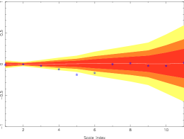
(c) Skewness

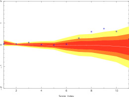
(d) Kurtosis

Figure 1: Spherical Mexican Hat wavelet coefficient statistics: Confidence regions derived from Monte Carlo simulations are shown for 68% (red), 95% (orange) and 99% (yellow) levels, as is the mean (solid white line).

 

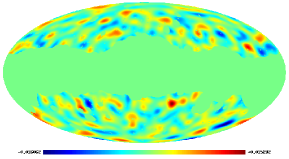
(a) Original coefficient map

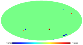
(b) Thresholded coefficient map

Figure 2: Spherical Mexican Hat wavelet coefficients at scale $a_{8}=250^{\prime}$: Those coefficients below $3\,\sigma(a_{8})$ are thresholded to zero so that likely deviations from Gaussianity may be localised on the CMB sky.

5 Conclusions and future work

A fast algorithm is presented and evaluated for performing a directional CSWT on the sphere. The fast implementation reduces the complexity of the CSWT by $\mathcal{O}(\sqrt{N_{\rm pix}})$, where $N_{\rm pix}$ is the number of pixels on the sphere. Furthermore, the numerical accuracy of the CSWT is improved by elegantly representing rotations in harmonic space.

The Gaussianity analysis of the WMAP 1-year data performed by Vielva et al.$\!{}^{{\bf?}}$ has been reproduced and confirmed using the fast CSWT. We consider the extension to a full directional analysis in an upcoming publication by McEwen et al.$\!{}^{{\bf?}}$; preliminary findings indicate deviations from Gaussianity outside of the 99% confidence level.

References

References

- [1] J.-P. Antoine and P. Vandergheynst, J. Math. Phys., 39, 8, 3987–4008. (1998).
- [2] D.M. Brink and G.R. Satchler, Angular Momentum (3rd Ed.), Clarendon Press, Oxford, (1993).
- [3] E. Komatsu et al., ApJ, 148, 119, (2003).
- [4] J.D. McEwen, M.P. Hobson, A.N. Lasenby and D.J. Mortlock, Preprint (astro-ph/0406604), submitted to MNRAS, (2004).
- [5] P. Vielva, E. Martinez-González, R.B. Barreiro, J.L. Sanz and L. Cayón, Preprint (astro-ph/0310273), submitted to ApJ, (2003).
- [6] B.D. Wandelt and K.M. Górski, Phys. Rev., 63, 123002, 1–6, (2001).