Searching for a holographic connection between dark energy and the low-$l$ CMB multipoles

Abstract

We consider the angular power spectrum in a finite universe with different boundary conditions and perform a fit to the CMB, LSS and supernova data. A finite universe could be the consequence of a holographic constraint, giving rise to an effective IR cutoff at the future event horizon. In such a model there is a cosmic duality relating the dark energy equation of state and the power spectrum, which shows a suppression and oscillatory behaviour that is found to describe the low $l$ features extremely well. However, much of the discussion here will also apply if we actually live inside an expanding bubble that describes our universe. The best fit to the CMB and LSS data turns out to be better than in the standard $\Lambda$CDM model, but when combined with the supernova data, the holographic model becomes disfavored. We speculate on the possible implications.

1 Introduction

The spatial geometry of the universe is known to be flat with $\Omega=1.02\pm 0.02$ [1, 2] so that even if the geometry is closed, one would argue that its radius should be much larger than the present Hubble scale. However, it is still possible that the universe is relatively small and finite. The simplest example is provided by a geometry which is not simply connected, such as a torus. In such a case the universe is effectively a box with periodic boundary conditions, resulting in suppression of power at large angular distances as well as in multiple images of the same sources in different directions. The present CMB data constrains the fundamental domain to be larger than 1.2 to 1.7 times the distance to the decoupling surface, depending on model assumptions [3].

A more subtle and potentially more far-reaching possibility is related to holography [4]. The holographic principle emerged first in the context of black holes, where it was noted that a local quantum field theory can not fully describe black holes while preserving unitarity; for a sufficiently large volume the entropy of an effective field theory will violate the Bekenstein bound [5]. This indicates that a local field theory overcounts the true dynamical degrees of freedom of a gravitating system. Therefore, an effective field theory which correctly accounts for the coarse grained interactions of the true dynamical degrees (e.g. strings), should be subject to global constraints that remove the overcounting. This should hold true also for a field theoretical description of the universe as a whole.

The issue then is, how would the holographic constraints manifest themselves in cosmology? At present no rigorous answer exists, but there are several phenomenological ideas [6]. For instance, it has been suggested that the effective field theory should exclude those degrees of freedom that will never be observed, giving rise to an IR cutoff $\tilde{L}$ at the future event horizon [7, 9, 10, 11, 12]. In a universe dominated by dark energy, the size of the future event horizon will tend to a constant which, given the WMAP results on dark energy, is of the order of $H^{-1}_{0}$, the present Hubble radius. Therefore, the consequences of such a cutoff could well be visible at the largest observable scales and in particular in the low CMB multipoles, where instead of continuous wave numbers one should deal with discrete ones even though, strictly speaking, the universe need not be finite.

In the case of topologically finite universes, the size of the universe correspond to a constant comoving size, which would be less that the Hubble radius during the inflationary epoch. This problem is also avoided if the effective cutoff is associated with the future event horizon which corresponds to an almost constant physical size and is never less than the Hubble radius.

The appearance of an IR cutoff may not be the only consequence of holography. An effective field theory that can saturate the Bekenstein bound will in general include states with a Schwarzschild radius much larger than the size of the cutoff volume. It seems reasonable that one should require [13, 14] that the energy in a given volume should not to exceed the energy of a black hole, which results in a constraint on the size of the zero point fluctuation, i.e. an effective UV cutoff. In that case the observations should reveal a correlation between dark energy and the power spectrum [12].

The universe constrained by holography is finite only in an effective, field theoretical sense. Therefore it is not obvious what sort of boundary conditions one should impose. In fact, periodic boundary conditions would appear to be the least natural. Instead, one could consider Dirichlet boundary conditions with quantum fields vanishing at the cutoff scale, or Neumann boundary conditions with vanishing derivatives ensuring that no currents flow beyond the cutoff. This bears some resembles to the “brick wall” model [15] or the “stretched horizon” model [16] of black holes, where one imposes a boundary condition for the fields on a plane close to the horizon. Also in the case where we actually live inside an expanding bubble, these choices of boundary conditions appear more natural. The choice of the boundary condition is important because it determines the way the wave numbers are discretized, which in turn makes a difference when fitting the actual data. Note also that many of the signatures of a finite universe considered in the literature, such as circles-in-the-sky, are specific to periodic boundary conditions.

No matter what the boundary conditions, the observable consequences of a holographic constraint would be likely to show up at the largest observable scales. Intriguingly enough, there are a number of features in the large angle CMB power spectrum, the most notorious being the suppression of the quadrupole and the octupole [1, 2]. In addition, there are some hints of an oscillatory behaviour of the power spectrum at low $l$ [17]. There has been attempts to explain these glitches by trans-Planckian physics [18, 19] and by models of multiple inflation [20]. While the suppressed quadrupole and octupoles can be explained by such models with modified primordial power spectra, the temperature-polarization power spectrum measured by WMAP is higher than expected and in general the fit to data cannot be significantly improved by modifying the primordial power spectrum [21]. The features seen at higher $l$ are even more difficult to fit by modifying the underlying power spectrum because they are very localized in $l$-space. It is therefore an interesting question whether the low $l$ features could actually tell us something about holography.

The purpose of the present paper is to consider a discrete power spectrum with different boundary conditions and make a fit to the CMB, the large scale structure (LSS) and supernova (SN) data. We pay a particular attention to the features in the power spectrum at low $l$. These considerations do not as such require holography but simply test the possible varieties of discreteness of the data as dictated by different boundary conditions. To relate this to the holographic ideas, we focus on a simple toy model [12] that links the equation of state of the dark energy to the features at low multipoles in the CMB power spectrum through an IR/UV cosmic duality.

The paper is organized as follows. In Sect. II we discuss the various boundary conditions and the procedure of discretization of the power spectrum. We deal primarily with Dirichlet and Neumann boundary conditions. In Sect. III we present the results of fits to the data, keeping the dark equation of state and the IR cutoff independent. In this way the results apply more generally, also to the case where we actually live inside a slowly expanding bubble. As an application to holography, in Sect. IV we consider a toy model of cosmic IR/UV duality [12] which predicts the equation of state for dark energy as a function of IR cutoff [8, 9]. Sect. V contains a discussion of the results.

2 Boundary Conditions

Let us start by assuming that the field theory contains an IR cutoff $\tilde{L}$, which we wish to translate into a cutoff at physical wavelengths. We will assume an isotropic universe so that the system is spherically symmetric. As a consequence of the IR cutoff the momenta $k$ will be discrete, but the allowed wave numbers will depend on the boundary conditions. However, if the discretization is due to a holographic constraint, there is no obvious way to choose one particular boundary condition over another. In the holographic case the cutoff $\tilde{L}$ is only effective: we do not live in any actual physical cavity and space can well be infinite, even if the effects are very similar to the effects of living inside a bubble. Rather, the nature of the boundary condition would be a manifestation of the holographic constraint itself and hence at the present phenomenological level undetermined. Therefore it makes sense to consider several likely possibilities.

Let us therefore consider quantization in a spherical potential well with infinitely high potential walls. The radial solutions for the wave functions are spherical Bessel functions with the ground state $j_{0}\propto\sin(kr)/kr$ with $r<r_{B}$, where $r_{B}$ is the radius of the spherical potential and is related to the IR cutoff. Imposing different boundary conditions on these solutions result in differences than can have observable consequences.

Periodic boundary conditions have been extensively discussed in the literature in the context of non-simply connected spaces. In general they lead to geometric patterns in the sky that are highly constrained by data [3]. For Cauchy boundary conditions, we would need to make model dependent assumptions about physics beyond the IR cutoff $\tilde{L}$, such as that the fields are exponentially suppressed for $r>\tilde{L}$. Therefore we prefer to focus on the unambiguous cases of the Dirichlet and Neumann boundary conditions.

2.1 Dirichlet

Requiring that the solution vanishes at $r=r_{B}$ one finds that the wavelength of the ground state is $\lambda_{c}=2r_{B}$. Thus the IR cutoff $\tilde{L}$ corresponds to a physical cutoff given by $\lambda_{c}=2\tilde{L}$.

For $x\gg 1$ we may write the Bessel function as $j_{l}(x)=\frac{1}{x}\sin\left(x-\frac{l\pi}{2}\right)$. Thus the allowed wavenumbers, $k_{nl}$, are determined by

$$j_{l}(k_{nl}r_{B})=\frac{1}{k_{nl}r_{B}}\sin\left(k_{nl}r_{B}-\frac{l\pi}{2}\right)=0~{},$$ (1)

which implies $k_{nl}r_{B}=\frac{l\pi}{2}+2\pi n$ for $n,l\in\mathcal{N}$, or

$$k_{nl}=\frac{1}{r_{B}}\left(\frac{l\pi}{2}+\pi n\right)~{}.$$ (2)

We emphasize that for each choice of the angular variable $l$, there is a different discrete set of the allowed momenta $k$.

2.2 Neumann

In this case we require the derivative of the allowed solutions vanish on the wall of the effective cavity defined by the IR cutoff so that there is no current flow out of the observable universe. The radial dependent part of the solutions is given by the spherical Bessel functions, so it amounts to requiring that the derivative of the spherical Bessel function vanishes on the wall of the bubble. Using the recurrence formulae for Bessel functions, one finds

$$\frac{d}{dx}j_{l}(x)=lx^{-1}j_{l}(x)-j_{l+1}(x)$$ (3)

so that the allowed momenta are defined by the condition

$$l(kr_{B})^{-1}j_{l}(kr_{B})-j_{l+1}(kr_{B})=0~{}.$$ (4)

for all $l,n\in\mathcal{N}$.

3 Discretization of the power spectrum

3.1 Preliminaries

In our case the discretization of the power spectrum differs from the more usual case of toroidal universes. Let us therefore repeat some of the basic steps involved in the discretization procedure.

We need to determine what is the proper relation between the discrete power spectrum and the usual continuous one. In a finite volume we can always expand a wave function $\psi(x)$ in terms of a complete set of orthonormal solutions to the equation of motion $u_{k}(x)$ so that $\psi(x)=\sum_{n}\psi_{n}u_{k_{n}}(x)$ with $\int|u_{k_{n}}(x)|^{2}dx=1~{}$ and $\psi_{n}=\int\psi(x)u_{k_{n}}^{*}(x)dx~{}.$ The probability of finding the state $\psi$ with momentum $k_{n}$ is then given by

$$P(k_{n})=|\psi_{n}|^{2}~{}.$$ (5)

The continuous limit is taken by letting the volume to go to infinity. The probability of finding the state $\psi$ with momentum in the interval between $k$ and $k+dk$ is then given by $P(k)dk=|\psi(k)|^{2}dk$ and

$$\psi(k)=\psi_{k}\sqrt{\frac{dN}{dk}}~{}$$ (6)

where $dN/dk$ is the density of states. By renormalizing $u_{k_{n}}(x)$ we may write $\psi(k)=\int\psi(x)u^{*}(k,x)dk$ where

$$u(k,x)=u_{k}(x)\sqrt{\frac{dN}{dk}}~{}.$$ (7)

Hence the continuous limit is reached by the replacement

$$\sum_{n}\to\int dN=\int dk\frac{dN}{dk}~{}.$$ (8)

In a spherically symmetric cavity, it is convenient to write the orthonormal solutions in the form

$$u_{nlm}(\vec{x})=A_{n}N_{l}j_{l}(kr)Y_{lm}(\theta,\phi)~{},$$ (9)

where $A_{n}^{2}$ is the density of states, $N_{l}$ is an $l$-dependent normalization factor; $r=|\vec{x}|$ and $\Omega_{x}=(\theta,\phi)$ is the angular direction of the coordinate $\vec{x}$. The normalization is chosen such that

$$\int_{0}^{L}drr^{2}\left[A_{n}N_{l}j_{l}(k_{n}r)\right]\left[A_{m}N_{l}j_{l}(k_{m}r)\right]=\delta_{nm}~{}.$$ (10)

According to the previous subsection, the continuous limit is taken by letting

$$\sum_{N}=\sum_{nlm}\to\int_{0}^{\infty}dk\frac{dn}{dk}\sum_{l}\sum_{m}~{}.$$ (11)

Using the convention

$$A_{n}^{2}=\frac{1}{2\pi}\frac{dk}{dn}~{},\qquad\delta_{nm}=2\pi A_{n}^{2}\delta(k_{n}-k_{m})~{},$$ (12)

then

$$\sum_{nlm}A_{n}^{2}\to\int_{0}^{\infty}\frac{dk}{2\pi}\sum_{l}\sum_{m}~{},$$ (13)

and the normalization factor becomes $N_{l}(k)=2k$. The expansion in terms of the eigenmode functions now reads

$$g(\vec{x})=\sum_{nlm}g_{nlm}u_{nlm}(\vec{x})=\sum_{nlm}g_{nlm}A_{n}N_{l}j_{l}(k_{n}r)Y_{lm}(\theta,\phi)~{},$$ (14)

where $u_{nlm}(\vec{x})$ is a solution to the equation of motion under the given boundary condition and the set $k_{n}$ is determined by the boundary condition.

As an example, consider the Dirichlet boundary condition which yields the constraint

$$u_{nlm}(\vec{x}_{B})=A_{n}N_{l}j_{l}(k_{n}r_{B})Y_{lm}(\theta,\phi)=0~{}.$$ (15)

It is clear that the allowed $k_{n}$’s depend on $l$ through the condition $j_{l}(k_{n}r_{B})=0$. Thus, instead of Eq. (14) we should write

$$g(\vec{x})=\sum_{nlm}g_{nlm}A_{nl}N_{l}j_{l}(k_{nl}r)Y_{lm}(\theta,\phi)~{},$$ (16)

where $k_{nl}$ is now the physical momentum depending on both $n$ and $l$. Note that in principle the amplitude $A$ can also depend on $l$. From Eq. (2) we find

$$A_{nl}^{2}=\frac{1}{2\pi}\frac{dk_{nl}}{dn}=\frac{1}{r_{B}}~{}.$$ (17)

Thus, very conveniently, for the Dirichlet boundary condition $A$ is actually independent of $l$ and $n$ in the large argument limit.

3.2 The discrete power spectrum

The power spectrum is defined as the power per log $k$ interval of the variance $\sigma_{g}^{2}$, given by

$$\sigma_{g}^{2}(\vec{x}) \equiv \left<g^{2}(\vec{x})\right>=\int d^{3}x~{}g^{2}(\vec{x})$$ (18)

$$= \int d^{3}x~{}\sum_{nlm}\sum_{n^{\prime}l^{\prime}m^{\prime}}\left<g^{*}_{nlm}g_{n^{\prime}l^{\prime}m^{\prime}}\right>u^{*}_{nlm}(\vec{x})u_{n^{\prime}l^{\prime}m^{\prime}}(\vec{x})=\sum_{nlm}\left<|g_{nlm}|^{2}\right>~{}.$$

Using the relation

$$g_{nlm}\equiv A_{nl}g_{lm}(k_{nl})=\frac{A_{nl}}{{\pi}N_{l}}k^{2}_{nl}i^{l}\int g(\vec{k}_{nl})Y_{lm}(\hat{k}_{nl})d\Omega_{k}~{},$$ (19)

in the continuum limit one finds that

$$\sigma_{g}^{2}(\vec{x})=\sum_{nlm}\left<|g_{nlm}|^{2}\right>$$

$$\to \int_{0}^{\infty}dk\sum_{lm}\frac{dn}{dk}A_{nl}^{2}\left<|g_{lm}(k)|^{2}\right>=\int_{0}^{\infty}\frac{dk}{2\pi}\sum_{lm}\left<|g_{lm}(k)|^{2}\right>$$

$$= \int_{0}^{\infty}\frac{dk}{2\pi}\sum_{lm}\frac{k^{4}}{\pi^{2}N^{2}_{l}}\int\int\left<|g(\vec{k})|^{2}\right>Y_{lm}^{*}(\hat{k}^{\prime})Y_{lm}(\hat{k})d\Omega_{k}d\Omega_{k^{\prime}}~{}.$$

Using the orthonormality relation $\sum_{lm}Y_{lm}(\theta,\phi)Y_{lm}^{*}(\theta^{\prime},\phi^{\prime})=\delta(\cos(\theta)-\cos(\theta^{\prime}))\delta(\phi-\phi^{\prime})$ and using $N_{l}(k)=2k$, we obtain the correct continuum expressions

$$\sigma_{g}^{2}(\vec{x})=\int_{0}^{\infty}\frac{dk}{(2\pi)^{3}}k^{2}\int d\Omega_{k}\left<|g(\vec{k})|^{2}\right>=\int_{0}^{\infty}\frac{dk}{k}\mathcal{P}_{g}(k)$$ (20)

with

$$\left<g^{*}(\vec{k})g(\vec{k}^{\prime})\right>=(2\pi)^{3}\delta^{3}(\vec{k}-\vec{k}^{\prime})\frac{2\pi^{2}}{k^{3}}\mathcal{P}_{g}(k)~{}.$$ (21)

3.3 The Sachs-Wolfe effect

The usual multipole expansion of the temperature anisotropies reads

$$\frac{\delta T}{T_{0}}(\theta,\phi)=\sum a_{lm}Y_{lm}(\theta,\phi)~{},$$ (22)

and the angular power spectrum is given by

$$C_{l}\equiv\frac{1}{2l+1}\sum_{m}<|a_{lm}|^{2}>~{}.$$ (23)

In a matter dominated universe, the Sachs-Wolfe effect $\delta T/T=-(1/5)\mathcal{R}$, implies

$$a_{lm}=\int d\Omega Y_{lm}^{*}(\theta,\phi)\frac{\delta T}{T_{0}}(\theta,\phi)=-\frac{1}{5}\int d\Omega_{x}Y_{lm}^{*}(\hat{x})\mathcal{R}(x_{dec}\hat{x})~{}.$$ (24)

Using

$$\mathcal{R}(\vec{x}_{dec})=\sum_{nlm}\mathcal{R}_{nlm}A_{nl}N_{l}j_{l}(k_{nl}r)Y_{lm}(\theta,\phi)~{},$$ (25)

and the definition

$$\left<R^{*}_{n^{\prime}l^{\prime}m^{\prime}}R_{nlm}\right>=\frac{2\pi^{2}}{k^{3}}\mathcal{P_{R}}(k)\delta_{nn^{\prime}}\delta_{ll^{\prime}}\delta_{mm^{\prime}}~{},$$ (26)

we obtain by a straightforward standard calculation the discrete version of the angular power spectrum as

$$C_{l}=\frac{1}{25}\sum_{n}A_{nl}^{2}\frac{2\pi^{2}}{k_{nl}^{3}}\mathcal{P_{R}}(k_{nl})N_{l}^{2}j^{2}_{l}(k_{nl}r)~{}.$$ (27)

Inserting $N_{l}^{2}=4k^{2}$ one obtains the usual continuum result $C_{l}=\frac{4\pi}{25}\frac{1}{2\pi^{2}}\int\frac{dk}{k}j_{l}^{2}(kr)\mathcal{P_{R}}(k)~{}.$ with $A_{nl}^{2}=\frac{1}{2\pi}dk/dn$.

Note that the set of the allowed momenta $k$ in the discrete version of the Sachs-Wolfe effect depends on $l$.

4 A toy model with IR/UV cosmic duality

In this section we outline the toy model of a cosmic CMB/dark energy duality put forward in [12]. In a universe dominated by dark energy in the asymptotic future we actually live inside a finite box, the so-called ”causal diamond” of the static de Sitter coordinates, which is bounded by the past and future event horizons [7]. In cosmic coordinates the finiteness could manifest itself as an effective IR regulator of the same order of magnitude as the future event horizon, which in a pure de Sitter space determines also the magnitude of the effective cosmological constant. If an IR/UV duality is at work in the theory at some fundamental level, the IR regulator might in some (complicated) way relate the dark energy and the IR cutoff of the CMB perturbation modes. The model of [12], that we explore here, might be considered as a simple toy model for such a connection

Let us now assume that the size of the IR cutoff is related to the the future event horizon $R_{H}=a\int_{t}^{\infty}{dt}/{a}$, i.e. the effective size of the universe is the one that we can ever hope to observe [7, 9, 10, 11, 12]. In other words, a local field theory should describe only the degrees of freedom that can ever be observed by a given observer. In a universe dominated by dark energy $R_{H}$ is of the order of the present Hubble radius $H_{0}^{-1}$ but the actual value depends on the equation of state of dark energy. We write the IR cutoff $\tilde{L}$ as

$$R_{H}\equiv c\tilde{L}~{},$$ (28)

where $c\sim{\cal O}(1)$ is a free parameter that will be related to dark energy. The connection comes about by requiring that he total energy in a region of spatial size $\tilde{L}$ should not exceed the mass of a black hole of the same size, or $\frac{4\pi}{3}\tilde{L}^{3}\rho_{\Lambda}\leq 4\pi\tilde{L}M_{P}^{2}$, where $\Lambda$ is the UV cutoff. The largest IR cutoff $\tilde{L}$ is obtained by saturating the inequality so that we write

$$\rho_{\Lambda}=3M_{P}^{2}\tilde{L}^{-2}=3c^{2}M_{P}^{2}R_{H}^{-2}~{}.$$ (29)

We adopt a flat universe with $\Omega=1$. Then from the Friedmann equation and Eq. (29) it follows that

$$R_{H}=a^{3/2}c\frac{1}{\sqrt{\Omega_{m}^{0}}H_{0}}\left(\frac{1-\Omega_{\Lambda}}{\Omega_{\Lambda}}\right)^{1/2}~{},$$ (30)

which implies that today the value of the future event horizon would be

$$R_{H}=\frac{c}{\sqrt{\Omega_{\Lambda}^{0}}}H_{0}^{-1}~{},$$ (31)

where the superscripts refer to the present values.

In flat space the multipole $l$ is given by $l=k_{l}(\eta_{0}-\eta_{*})$ where $\eta_{0}-\eta_{*}$ is the comoving distance to the last-scattering surface and $k_{l}$ is the corresponding comoving wave number. The comoving distance to last scattering is given by

$$\eta_{0}-\eta_{*}=\int_{0}^{z_{*}}dz^{\prime}\frac{1}{H(z^{\prime})}$$ (32)

and if the dominant energy components are dark energy and matter, then $H^{2}(z)=H_{0}^{2}\left[\Omega_{\Lambda}^{0}(1+z)^{(3+3w)}+(1-\Omega_{\Lambda}^{0})(1+z)^{3}\right]~{},$ where $w$ is given by the equation of state of dark energy $p_{\Lambda}=w\rho_{\Lambda}$. Here $w$ is not a free parameter but is related to the constant $c$ through [9]

$$w=-\frac{1}{3}-\frac{2}{3c}\sqrt{\Omega_{\Lambda}}~{}.$$ (33)

This equation also holds at the present so that

$$w_{0}=-\frac{1}{3}-\frac{2}{3c}\sqrt{\Omega_{\Lambda}^{0}}~{}.$$ (34)

Thus, the distance to last scattering is a function of $w$ which can be found by fixing the free parameter $c$. Since $\tilde{L}$ does not depend on $c$, one finds with Dirichlet boundary condition [12] $\tilde{L}=1.2\times H_{0}^{-1}$ or $k_{c}\equiv\lambda_{c}/(2\pi)=1.2/\pi\times H_{0}^{-1}$, where $k_{c}$ defines the smallest allowed wave number. But because the distance to last scattering depends on $w$, the relative position of the cutoff in the CMB spectrum depends on $w$.

Testing this model means fitting simultaneously the power spectrum and $w$, using different boundary conditions. This yields the value of $c$, which is the only free parameter here: the shape of the power spectrum is fixed once $c$ (and the boundary condition) is fixed. Note that because the space is effectively finite, there will be oscillations at low $l$ in the power spectrum. These oscillations are however not freely adjustable but depend on the equation of state of dark energy, making the holographic toy model highly constrained and predictive.

However, given that we do not know exactly how the boundary condition should be imposed, we allow for more freedom in our fits to data. Instead of fixing the infrared cut-off at $k_{c}\equiv\lambda_{c}/(2\pi)=1.2/\pi\times H_{0}^{-1}$ we take it to be a free parameter $k_{\rm cut}$. As it turns out the best fit is at $k_{\rm cut}\sim 0.5-0.6k_{c}$, and given our ignorance of how to impose the boundary condition this is an approximation at the same level as choosing different types of boundaries (Neumann, Dirichlet, etc.). This leaves us with two parameters for any given model (in addition to the choice of boundary condition): $c$ and $k_{\rm cut}$. In the following section we present a likelihood analysis of the model using CMB, LSS, and SNI-a data.

5 Data analysis

5.1 The procedure

In order to test the discrete models against data we employ the following procedure: First a boundary condition (Dirichlet or Neumann in our case) is chosen. Next we calculate $\chi^{2}$ for each set of $c$ and $k_{\rm cut}$, while marginalizing over all other cosmological parameters. As our framework we choose the minimum standard model with 6 parameters: $\Omega_{m}$, the matter density, $\Omega_{b}$, the baryon density, $H_{0}$, the Hubble parameter, and $\tau$, the optical depth to reionization. The normalization of both CMB and LSS spectra are taken to be free and unrelated parameters. The priors we use are given in Table 1.

Table 1: Priors on cosmological parameters used in the likelihood analysis.

Parameter	Prior	Distribution
$\Omega=\Omega_{m}+\Omega_{X}$	1	Fixed
$h$	$0.72\pm 0.08$	Gaussian [23]
$\Omega_{b}h^{2}$	0.014–0.040	Top hat
$n_{s}$	0.6–1.4	Top hat
$\tau$	0–1	Top hat
$Q$	—	Free
$b$	—	Free

Likelihoods are calculated from $\chi^{2}$ so that for 1 parameter estimates, 68% confidence regions are determined by $\Delta\chi^{2}=\chi^{2}-\chi_{0}^{2}=1$, and 95% region by $\Delta\chi^{2}=4$. $\chi_{0}^{2}$ is $\chi^{2}$ for the best fit model found. In 2-dimensional plots the 68% and 95% regions are formally defined by $\Delta\chi^{2}=2.30$ and 6.17 respectively. Note that this means that the 68% and 95% contours are not necessarily equivalent to the same confidence level for single parameter estimates.

5.2 Description of the data sets

• Supernova luminosity distances

  We perform our likelihood analysis using the “gold” dataset compiled and described in Riess et al [31] consisting of 157 SNe Ia using a modified version of the SNOC package [32].

• Large Scale Structure (LSS).

  At present there are two large galaxy surveys of comparable size, the Sloan Digital Sky Survey (SDSS) [26, 25] and the 2dFGRS (2 degree Field Galaxy Redshift Survey) [24]. Once the SDSS is completed in 2005 it will be significantly larger and more accurate than the 2dFGRS. In the present analysis we use data from SDSS, but the results would be almost identical had we used 2dF data instead. In the data analysis we use only data points on scales larger than $k=0.15h$/Mpc in order to avoid problems with non-linearity.

• Cosmic Microwave Background.

  The CMB temperature fluctuations are conveniently described in terms of the spherical harmonics power spectrum $C_{l}^{TT}\equiv\langle|a_{lm}|^{2}\rangle$, where $\frac{\Delta T}{T}(\theta,\phi)=\sum_{lm}a_{lm}Y_{lm}(\theta,\phi)$. Since Thomson scattering polarizes light, there are also power spectra coming from the polarization. The polarization can be divided into a curl-free $(E)$ and a curl $(B)$ component, yielding four independent power spectra: $C_{l}^{TT}$, $C_{l}^{EE}$, $C_{l}^{BB}$, and the $T$-$E$ cross-correlation $C_{l}^{TE}$.

  The WMAP experiment has reported data only on $C_{l}^{TT}$ and $C_{l}^{TE}$ as described in Refs. [1, 2, 27, 28, 29]. We have performed our likelihood analysis using the prescription given by the WMAP collaboration [2, 27, 28, 29] which includes the correlation between different $C_{l}$’s. Foreground contamination has already been subtracted from their published data.

5.3 Results

First, we perform the likelihood analysis separately for the CMB+LSS data and the SNIa data. In Fig. 1 we show the likelihood in $c,k_{\rm cut}$ space for the Dirichlet boundary condition. The best fit model has $\chi^{2}=1444.8$ as opposed to the best fit $\Lambda$CDM model which has $\chi^{2}=1447.5$.

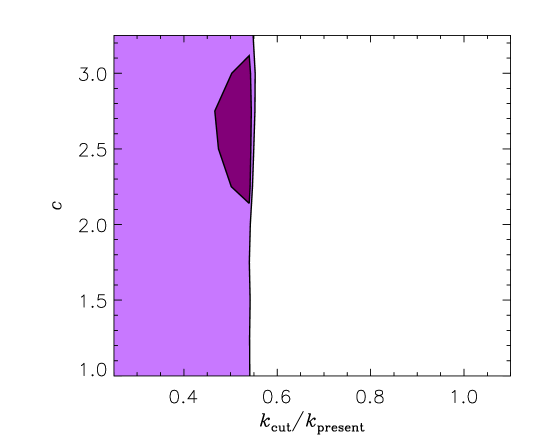
Figure 1: 68% (dark) and 95% (light) likelihood contours for WMAP and SDSS data using the Dirichlet boundary condition.

In Fig. 2 we show the same analysis, but for the Neumann boundary condition. Here, the best fit is $\chi^{2}=1441.4$, somewhat better than for the previous case.

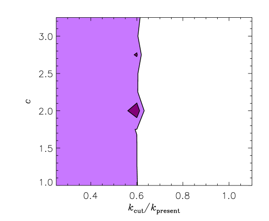
Figure 2: 68% (dark) and 95% (light) likelihood contours for WMAP and SDSS data using the Neumann boundary condition.

In Fig. 3 we show CMB temperature power spectra for the two best fit models [30]. Interestingly, the curve with Neumann boundary conditions is able to fit the small $l$ spectrum oscillations almost perfectly, including the $l\sim 20$ feature. However, the $l\sim 40$ feature is not reproduced. In both cases the power spectrum suppression at small $l$ is reproduced nicely because of the large scale cut-off in the spectrum.

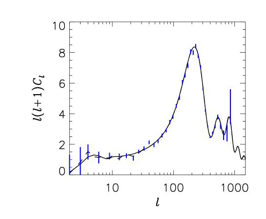
Figure 3: Temperature power spectra for the two best fit models, the full line is with Dirichlet boundary conditions and the dashed with Neumann boundary conditions. The data shown is the binned WMAP data.

Fig. 4 show the same analysis performed for the SNIa data. In this case there is no dependency on the cut-off scale, only on $c$, because that parameter modifies the dark energy behaviour. The best fit is at $\chi^{2}=177.1$ which is almost identical to that of the best fit $\Lambda$CDM model.

However, as can be seen, the best fits of CMB+LSS and SNIA are incompatible. This is illustrated in Fig. 5 which shows a combined CMB+LSS+SNIa fit for the Dirichlet boundary condition. Here, the best fit is at $\chi^{2}=1636.8$, as opposed to the best fit $\Lambda$CDM model which has $\chi^{2}=1626.4$. The fundamental reason for the discrepancy is just the well-known degeneracy between the matter density and the dark energy equation of state, $w$. If only CMB and LSS data is considered, then having $w>-1$ generally requires a higher matter density, whereas for SNIa data the reverse is true. This means that the combination in general rules out any model with a $w$ which is too high. For a constant $w$ the present bound is $w\leq-0.79$ at 95% C.L. [22].

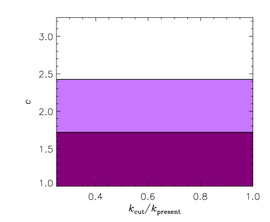
Figure 4: 68% (dark) and 95% (light) likelihood contours for SNIa data.

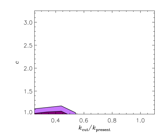
Figure 5: 68% (dark) and 95% (light) likelihood contours for WMAP, SDSS and SNIa data.

6 Discussion

It is intriguing that with the holographic toy model of Sect. 4 the power spectrum and in particular the low $l$ features are automatically fitted almost perfectly, as can be gathered from Fig. 3. The CMB and LSS data, on its own, would indeed be consistent with an IR/UV cosmic duality with an IR cutoff. However, from the analysis that combined CMB and LSS with the supernova data the conclusion clearly seems to be that in its present form the toy model of cosmic duality is strongly disfavored.

In fact, it would have been a great surprise if such a simple toy model would have worked perfectly as the actual holographic constraint is expected to be rather complicated. It is even conceivable that it manifests itself in different ways at different length scales. From a holographic point of view, supernova luminosity effects represent ordinary local physics and therefore have a different status from dark energy measured by CMB, which is a more global concept. It is also possible that the apparent decrease in the distant supernova luminosities is not due to accelerated expansion but to some other physical process. An example would be the recently suggested axion-photon mixing [33].

That said, one should note that if we use, for the cutoff on the large scale CMB anisotropies, the future event horizon at last scattering [12], then with $c=2$ and $\Omega_{\Lambda}^{0}=0.7$ corresponding to $w_{0}=-0.61$, the toy model with CMB/dark energy duality implies $k_{cut}/k_{present}=0.6$. Curiously that is in the maximum likelihood region with Neumann boundary conditions (see Fig. 2).

The present holographic model presents one possibility of how new physics might effect present day cosmology; some others have been discussed in light of observational data in [19]. Although no firm conclusions can be drawn at this stage, it is nevertheless encouraging that data is good enough for testing these ideas. Signals for a discrete power spectrum and a holographic connection between the ultraviolet and the infrared remain interesting possibilities linked to fundamental physics that are worth searching for also in the forthcoming cosmological data.

References

References

- [1] C. L. Bennett et ll., Astrophys. J. Suppl. 148, 1 (2003) [arXiv:astro-ph/0302207];
- [2] D. N. Spergel et al. [WMAP Collaboration], Astrophys. J. Suppl. 148, 175 (2003) [arXiv:astro-ph/0302209].
- [3] N. J. Cornish, D. N. Spergel, G. D. Starkman and E. Komatsu, Phys. Rev. Lett. 92, 201302 (2004) [arXiv:astro-ph/0310233]; N. G. Phillips and A. Kogut, arXiv:astro-ph/0404400.
- [4] G. ’t Hooft, gr-qc/9310026. L. Susskind, J. Math. Phys. 36, 6377 (1995) [hep-th/9409089]; R. Bousso, Rev. Mod. Phys. 74, 825 (2002) [hep-th/0203101].
- [5] J. D. Bekenstein, Phys. Rev. D 7 (1973) 2333.
- [6] A. Strominger, JHEP 0111, 049 (2001) [hep-th/0110087]; V. Balasubramanian, J. de Boer and D. Minic, Phys. Rev. D 65, 123508 (2002) [hep-th/0110108]; T. Banks and W. Fischler, hep-th/0111142; C. J. Hogan, Phys. Rev. D 66, 023521 (2002) [astro-ph/0201020]; F. Larsen, J. P. van der Schaar and R. G. Leigh, JHEP 0204, 047 (2002) [hep-th/0202127]; A. Albrecht, N. Kaloper and Y. S. Song, hep-th/0211221; U. H. Danielsson, JCAP 0303, 002 (2003) [hep-th/0301182]; E. Keski-Vakkuri and M. S. Sloth, JCAP 0308, 001 (2003) [hep-th/0306070]; J. P. van der Schaar, JHEP 0401, 070 (2004) [hep-th/0307271]; T. Banks and W. Fischler, hep-th/0310288; C. J. Hogan, astro-ph/0310532; F. Larsen and R. McNees, hep-th/0402050.
- [7] T. Banks, hep-th/0007146; R. Bousso, JHEP 0011, 038 (2000) [hep-th/0010252]; T. Banks and W. Fischler, hep-th/0102077; L. Dyson, M. Kleban and L. Susskind, JHEP 0210, 011 (2002) [hep-th/0208013]; M. K. Parikh, I. Savonije and E. Verlinde, Phys. Rev. D 67, 064005 (2003) [hep-th/0209120]; N. Kaloper, M. Kleban, A. Lawrence, S. Shenker and L. Susskind, JHEP 0211, 037 (2002) [hep-th/0209231]; T. Banks, W. Fischler and S. Paban, JHEP 0212, 062 (2002) [hep-th/0210160]; U. H. Danielsson, D. Domert and M. Olsson, Phys. Rev. D 68, 083508 (2003) [hep-th/0210198]; A. Albrecht and L. Sorbo, hep-th/0405270; B. Freivogel and L. Susskind, arXiv:hep-th/0408133.
- [8] S. D. H. Hsu, hep-th/0403052.
- [9] M. Li, hep-th/0403127.
- [10] Q. G. Huang and M. Li, astro-ph/0404229.
- [11] Q. G. Huang and Y. G. Gong, astro-ph/0403590.
- [12] K. Enqvist and M. S. Sloth, Phys. Rev. Lett. 93, 221302 (2004) [hep-th/0406019].
- [13] A. G. Cohen, D. B. Kaplan and A. E. Nelson, Phys. Rev. Lett. 82, 4971 (1999) [hep-th/9803132].
- [14] S. Thomas, Phys. Rev. Lett. 89, 081301 (2002).
- [15] G. ’t Hooft, Nucl. Phys. B 256, 727 (1985).
- [16] L. Susskind, L. Thorlacius and J. Uglum, Phys. Rev. D 48, 3743 (1993) [arXiv:hep-th/9306069].
- [17] D. Tocchini-Valentini, M. Douspis and J. Silk, arXiv:astro-ph/0402583.
- [18] J. Martin and C. Ringeval, Phys. Rev. D 69, 083515 (2004) [arXiv:astro-ph/0310382]; J. Martin and C. Ringeval, Phys. Rev. D 69, 127303 (2004) [arXiv:astro-ph/0402609].
- [19] S. Hannestad and L. Mersini-Houghton, hep-ph/0405218 (to appear in Phys. Rev. D).
- [20] P. Hunt and S. Sarkar, arXiv:astro-ph/0408138.
- [21] S. Hannestad, JCAP 0404, 002 (2004) [astro-ph/0311491].
- [22] S. Hannestad and E. Mortsell, JCAP 0409, 001 (2004) [astro-ph/0407259].
- [23] W. L. Freedman et al., Astrophys. J. 553, 47 (2001) [arXiv:astro-ph/0012376].
- [24] M. Colless et al., astro-ph/0306581.
- [25] M. Tegmark et al. [SDSS Collaboration], astro-ph/0310723.
- [26] M. Tegmark et al. [SDSS Collaboration], astro-ph/0310725.
- [27] L. Verde et al., Astrophys. J. Suppl. 148 (2003) 195 [astro-ph/0302218].
- [28] A. Kogut et al., Astrophys. J. Suppl. 148 (2003) 161 [astro-ph/0302213].
- [29] G. Hinshaw et al., Astrophys. J. Suppl. 148 (2003) 135 [astro-ph/0302217].
- [30] U. Seljak and M. Zaldarriaga, Astrophys. J. 469 (1996) 437 [astro-ph/9603033]. See also the CMBFAST website at http://www.cmbfast.org
- [31] A. G. Riess et al. [Supernova Search Team Collaboration], Astrophys. J. 607, 665 (2004) [arXiv:astro-ph/0402512].
- [32] Goobar, A., Mörtsell, E., Amanullah, R., Goliath, M., Bergström, L. and Dahlén, T., 2002, Astron. Astrophys., 392, 757 [astro-ph/0206409]. Code available at http://www.physto.se/ariel/snoc/
- [33] C. Csaki, N. Kaloper and J. Terning, Phys. Rev. Lett. 88, 161302 (2002) [hep-ph/0111311]; C. Deffayet, D. Harari, J. P. Uzan and M. Zaldarriaga, Phys. Rev. D 66, 043517 (2002) [arXiv:hep-ph/0112118]; C. Csaki, N. Kaloper and J. Terning, Phys. Lett. B 535, 33 (2002) [arXiv:hep-ph/0112212]; E. Mortsell, L. Bergstrom and A. Goobar, Phys. Rev. D 66, 047702 (2002) [arXiv:astro-ph/0202153]; M. Christensson and M. Fairbairn, Phys. Lett. B 565, 10 (2003) [arXiv:astro-ph/0207525]; E. Mortsell and A. Goobar, JCAP 0304, 003 (2003) [arXiv:astro-ph/0303081].