Bayesian Statistics and Parameter Constraints on the
Generalized Chaplygin Gas Model using SNe Ia Data

Abstract

The type Ia supernovae (SNe Ia) observational data are used to estimate the parameters of a cosmological model with cold dark matter and the generalized Chaplygin gas model (GCGM). The GCGM depends essentially on five parameters: the Hubble constant, the parameter $\bar{A}$ related to the velocity of the sound, the equation of state parameter $\alpha$, the curvature of the Universe and the fraction density of the generalized Chaplygin gas (or the cold dark matter). The parameter $\alpha$ is allowed to take negative values and to be greater than $1$. The Bayesian parameter estimation yields $\alpha=-0.86^{+6.01}_{-0.15}$, $H_{0}=62.0^{+1.32}_{-1.42}\,km/Mpc.s$, $\Omega_{k0}=-1.26_{-1.42}^{+1.32}$, $\Omega_{m0}=0.00^{+0.86}_{-0.00}$, $\Omega_{c0}=1.39^{+1.21}_{-1.25}$, $\bar{A}=1.00^{+0.00}_{-0.39}$, $t_{0}=15.3^{+4.2}_{-3.2}$ and $q_{0}=-0.80^{+0.86}_{-0.62}$, where $t_{0}$ is the age of the Universe and $q_{0}$ is the value of the deceleration parameter today. Our results indicate that a Universe completely dominated by the generalized Chaplygin gas is favoured, what reinforces the idea that the this gas may unify the description for dark matter and dark energy, at least as the SNe Ia data is concerned. A closed and accelerating Universe is also favoured. The traditional Chaplygin gas model (CGM), $\alpha=1$ is not ruled out, even if it does not give the best-fitting. Particular cases with four or three independent free parameters are also analysed.

PACS number(s): 98.80.Bp, 98.80.Es, 04.60.Gw

1 Introduction

One of the most important problems today in cosmology is the nature of dark matter and dark energy that must dominate the matter content of the Universe [1]. The existence of dark matter is suggested by the anomalies in the dynamics of galaxies and clusters of galaxies [2]. Dark energy seems to be an inevitable consequence of the present acceleration of the Universe as indicated by the type Ia supernovae (SNe Ia) data, which asks for a fluid of negative pressure which does not agglomerate at small scales [3, 4]. While in general the nature of dark matter can be connected with relics of fundamental theories, like axions [5], there are two main candidates to represent dark energy: cosmological constant [6] and quintessence which is a self interacting scalar field [7]–[9]. Both models suffers of many drawbacks, mainly linked with fine tuning of parameters, as in the quintessence model [10], or disagreement with the theoretically predicted values, like in the cosmological constant case [11].

The traditional Chaplygin gas model (CGM) and the generalized Chaplygin gas model (GCGM) have been widely considered as alternatives to the cosmological constant and to quintessence as the dark energy that drives the present acceleration of the Universe [12]–[15]. The appealing of the GCGM comes from, among other reasons, the fact that it can unify the description of dark matter and dark energy. The generalized Chaplygin gas (GCG) is characterized by the equation of state

$$p=-\frac{A}{\rho^{\alpha}}\quad,$$ (1)

where $A$ and $\alpha$ are constants that in general are considered as positive numbers. The conservation equation leads to the relation

$$\rho=\biggr{\{}A+\frac{B}{a^{3(1+\alpha)}}\biggl{\}}^{1/(1+\alpha)}\quad.$$ (2)

Some of the main interesting features of eq. (2) are the following. Initially, the GCGM behaves as a dust fluid, with $\rho\propto a^{-3}$, while at late times the GCGM behaves as a cosmological constant term, $\rho\propto A^{1/(1+\alpha)}$. Hence, the GCGM interpolates a matter dominated phase (where the formation of structure can happen) and a de Sitter phase. At the same time, the sound velocity of the GCGM is positive which assures that, in spite of exhibiting a negative pressure, it is stable against perturbations of the background configuration [16].

A lot of effort has been done in order to constrain the free parameters of the GCGM. Type Ia supernovae data [17]–[26], the spectra of anisotropy of cosmic microwave background radiation [27], the mass power spectrum [28, 29, 30], gravitational lenses [31], X-ray data [32] and age estimates of high-$z$ objects [33] have extensively been used in this sense. This is essential for many obvious reasons. One of them is that if the parameter $\alpha$ is close to zero, the GCGM reduces essentially to the cosmological constant model. If observations indicate that this is the preferred value, the appealing for the cosmological constant as dark energy is reinforced. In a previous work [17], we have analysed the case of the traditional Chaplygin gas model, where $\alpha=1$, using the SNe Ia data. One important aspect of this analysis is the use of the Bayesian statistics, for one side, and also the fact that all free parameters (Hubble constant, the curvature term, the value of the sound velocity and the proportion of ordinary matter and Chaplygin gas) of the model were taken into account in the treatment of the problem. This contrasts with most of the analyses previously found in the literature in the sense that they employ a more simplified statistical analysis or some input parameters were fixed a priori [18]–[26]. In that work [17], it was concluded that the unification scenario (i.e., without pressureless matter), and a sound velocity near (but not equal) to the velocity of light were preferred. Moreover, a closed Universe was clearly favoured.

The aim of the present work is to apply the same analysis, using the Bayesian statistics and taking into account all free parameters, to the GCGM. In order to keep contact with the previous work, we will use the same supernovae sample. This sample is much smaller than those available today (see, for example, ref. [34]–[36]). But, the quality of the data is extremely good, which leads to a smaller value of $\chi_{\nu}^{2}$ (the quantity that measures the quality of the fitting): with this restricted sample the best-fitting gives $\chi_{\nu}^{2}$ around $0.74$, while for the complete “gold” sample [34], the value mounts to unity. In the GCGM there are five free parameters instead of the four free parameters of the traditional Chaplygin gas model ($\alpha=1$): the Hubble constant $H_{0}$, the parameter $\bar{A}$ related to the sound velocity of the Chaplygin gas, the curvature density parameter $\Omega_{k0}$, the ordinary matter parameter $\Omega_{m0}$ (or alternatively, the Chaplygin gas parameter $\Omega_{c0}$) and the equation of state parameter $\alpha$.

One important point in performing this generalized analysis is the range of validity of the parameter $\alpha$. Usually, it has been assumed that $0\leq\alpha\leq 1$. The reason is twofold: $\alpha$ greater than one could lead, even if in the future, to a sound velocity greater than the velocity of the light; $\alpha$ negative should lead to an imaginary sound velocity, that is, instability. However, an analysis of the supernovae data may taken into account values of $\alpha$ greater than one or negative. In particular, in reference [25], using a different statistical approach with respect to the method employed here, a value of $\alpha$ near $2$ was favoured. In fact, values of $\alpha$ outside that limited range can be considered. The reason lies in the fact that the GCGM with the equation of state (1) may be a phenomenological manifestation of a theory expressed in terms, for example, of scalar field with a potential, or even of tachyon condensate model [37, 38]. In this case, the notion of sound velocity can not be identified with the ordinary expression used in the perfect fluid approach, and no violation of causality or instability may occur if $\alpha$ is greater than one or negative.

Hence, in our analysis the parameter $\alpha$ will vary from negative to highly positive values. The prediction for each parameter ($\alpha$, $H_{0}$, $\Omega_{k0}$, $\Omega_{m0}$, $\Omega_{c0}$ and $\bar{A}$) is taken marginalizing, i.e., integrating over the other parameters. We stress that such marginalization procedure gives predictions that can be quite different from a two dimensional analysis, for example, where one searches for the simultaneous preferred values for any two parameters. This marginalization is in fact essential in order to have the correct prediction for a given free parameter. We will consider the following cases: all five parameters free; spatial curvature zero (four free parameters); pressureless matter given only by the barionic component (four free parameters); pressureless matter absent (four free parameters); spatial curvature zero and no pressureless matter component (three free parameters); spatial curvature zero and pressureless matter component given by the barionic component (three free parameteres). For the more general case with five free parameters the predictions we obtain are the following: $\alpha=-0.86_{-0.15}^{+6.01}$, $H_{0}=62.0_{-1.42}^{+1.32}\,km/Mpc.s$, $\Omega_{k0}=-1.26_{-1.42}^{+1.32}$, $\Omega_{m0}=0.00_{-0.00}^{+0.86}$, $\Omega_{c0}=1.39_{-1.25}^{+1.21}$, $\bar{A}=1.00_{-0.39}^{+0.00}$. Moreover the predicted age of the Universe and the value of de deceleration parameter today are $t_{0}=15.3_{-3.2}^{+4.2}$ and $q_{0}=-0.80_{-0.62}^{+0.86}$, respectively. The results are consistent with, for example, the age of globular clusters [39]. Two crucial parameters are $\alpha$ and $\bar{A}$, since if $\alpha=0$ and/or $\bar{A}=1$ are favoured, the GCGM becomes equivalent to the cosmological constant model ($\Lambda$CDM). The value of the parameter $\bar{A}$ is in fact peaked at unity. But for reasons discussed later, this does not imply that this is the most favoured value; indeed it is just expected to be near unity. On the other hand, the parameter $\alpha$ is peaked in a negative value, but the spread is very large. In particular, the traditional Chaplygin gas with $\alpha=1$ can not be excluded or even disfavoured: in most of the cases this value of $\alpha$ is favoured with a probability around $50\%$. Hence, our analysis does not exclude the traditional Chaplygin gas model.

This paper is organized as follows. In next section, the basic equations and quantities are exhibited. Section $3$ explains the type Ia supernovae fitting. In section $4$, we display the results of the Bayesian analysis of type Ia supernovae data with the GCGM. We present our conclusions in section $5$.

2 Description of the GCG model

Regardless the possibility of unification of dark matter and dark energy using the GCGM, we will consider a model for the Universe today with two fluids: pressureless matter and the GCG. In doing so, our aim is to verify whether the unified model is the case favoured by observations. Moreover, even if in the GCGM there is no need of a dark matter component, there is baryonic matter in the Universe which is represented also by a pressureless matter. Hence, the dynamics of the Universe is driven by the Friedmann’s equation

$$\biggr{(}\frac{\dot{a}}{a}\biggl{)}^{2}+\frac{k}{a^{2}} = \frac{8\pi G}{3}\biggr{(}\rho_{m}+\rho_{c}\biggl{)}\quad,$$ (3)

$$\dot{\rho}_{m}+3\frac{\dot{a}}{a}\rho_{m} = 0\quad,$$ (4)

$$\dot{\rho}_{c}+3\frac{\dot{a}}{a}\biggr{(}\rho_{c}-\frac{A}{\rho_{c}^{\alpha}}\biggl{)} = 0\quad,$$ (5)

where $\rho_{m}$ and $\rho_{c}$ stand for the pressureless matter and generalized Chaplygin gas component. Dot means derivative with respect to the cosmic time $t$. As usual, $k=0,1,-1$ indicates a flat, closed and open spatial section. In the conservation equation for the generalized Chaplygin gas component (5), the equation of state (1) has been introduced.

The equations expressing the conservation law for each fluid (4)-(5) lead to

$$\rho_{m}=\frac{\rho_{m0}}{a^{3}}\quad,\quad\rho_{c}=\biggr{\{}A+\frac{B}{a^{3(1+\alpha)}}\biggl{\}}^{1/(1+\alpha)}\quad,$$ (6)

Henceforth, we will parametrize the scale factor such that its value today is equal to unity, $a_{0}=1$. Hence, $\rho_{m0}$ and $\rho_{c0}=\biggr{\{}A+B\biggl{\}}^{1/(1+\alpha)}$ are the pressureless matter and GCG densities today. Eliminating from the last relation the parameter $B$, the GCG density at any time can be reexpressed as

$$\rho_{c}=\rho_{c0}\biggr{\{}\bar{A}+\frac{1-\bar{A}}{a^{3(1+\alpha)}}\biggl{\}}^{1/(1+\alpha)}\quad,$$ (7)

where $\bar{A}=A/\rho_{c0}$. This parameter $\bar{A}$ is connected with the sound velocity for the GCG today by the relation $v_{s}^{2}=\alpha\bar{A}$.

The luminosity distance is given by the expression

$$D_{L}=\frac{a_{0}^{2}}{a}r_{1}\quad,$$ (8)

$r_{1}$ being the co-moving coordinate of the source. Using the expression for the propagation of light

$$ds^{2}=0=dt^{2}-\frac{a^{2}dr^{2}}{1-kr^{2}}\quad,$$ (9)

and the Friedmann’s equation (3), we can reexpress the luminosity distance as

$$D_{L}=(1+z)S[f(z)]\quad,$$ (10)

where

$$S(x)=x\quad(k=0),\quad S(x)=\sin x\quad(k=1),\quad S(x)=\sinh x\quad(k=-1)\quad,$$ (11)

and

$$f(z)=\frac{1}{H_{0}}\int_{0}^{z}\frac{d\,z^{\prime}}{\{\Omega_{m0}(z^{\prime}+1)^{3}+\Omega_{c0}[\bar{A}+(z^{\prime}+1)^{3(1+\alpha)}(1-\bar{A})]^{1/(1+\alpha)}-\Omega_{k0}(z^{\prime}+1)^{2}\}^{1/2}}\quad,$$ (12)

with the definitions

$$\Omega_{m0}=\frac{8\pi G}{3}\frac{\rho_{m0}}{H_{0}^{2}}\quad,\quad\Omega_{c0}=\frac{8\pi G}{3}\frac{\rho_{c0}}{H_{0}^{2}}\quad,\quad\Omega_{k0}=-\frac{k}{H_{0}^{2}}\quad,$$ (13)

where $\Omega_{m0}+\Omega_{c0}+\Omega_{k0}=1$. The final equations have been also expressed in terms of the redshift $z=-1+\frac{1}{a}$.

The age of the Universe today can be expressed as

$$\frac{t_{0}}{T}=\int_{0}^{z}\frac{d\,z^{\prime}}{(1+z^{\prime})\{\Omega_{m0}(z^{\prime}+1)^{3}+\Omega_{c0}[\bar{A}+(z^{\prime}+1)^{3(1+\alpha)}(1-\bar{A})]^{1/(1+\alpha)}-\Omega_{k0}(z^{\prime}+1)^{2}\}^{1/2}}\quad,$$ (14)

where $T=(100/H_{0})\times 10^{10}$, so $t_{0}$ has units of years.

The value of the decelerated parameter today, $q_{0}=-\frac{a\ddot{a}}{\dot{a}^{2}}$, is given by

$$q_{0}=\frac{\Omega_{m0}+\Omega_{c0}(1-3\bar{A})}{2}\quad.$$ (15)

The value $a_{i}$ of the scale factor that shows the beginning of the recent accelerating phase of the Universe is given by the roots of the equation

$$\ddot{a}=a(\dot{H}+H^{2})\quad,$$ (16)

and is related to the redshift value $z_{i}$ such that $\frac{a_{i}}{a_{0}}=\frac{1}{1+z_{i}}$ or $z_{i}=-1+\frac{a_{0}}{a_{i}}$.

3 Supernovae fitting

We proceed by fitting the SNe Ia data using the GCG model described above. Essentially, we compute the quantity distance moduli,

$$\mu_{0}=5\log\left(\frac{D_{L}}{M\!pc}\right)+25\quad,$$ (17)

and compare the same distance moduli as obtained from observations. The quality of the fitting is characterized by the $\chi^{2}$ parameter of the least-squares statistic, as defined in Ref. [3],

$$\chi^{2}=\sum_{i}\frac{\left(\mu_{0,i}^{o}-\mu_{0,i}^{t}\right)^{2}}{\sigma_{\mu_{0},i}^{2}+\sigma_{mz,i}^{2}}\quad.$$ (18)

In this expression, $\mu_{0,i}^{o}$ is the measured value, $\mu_{0,i}^{t}$ is the value calculated through the model described above, $\sigma_{\mu_{0},i}^{2}$ is the measurement error, $\sigma_{mz,i}^{2}$ is the dispersion in the distance modulus due to the dispersion in galaxy redshift due to peculiar velocities. This quantity we will taken as

$$\sigma_{mz}=\frac{\partial\log D_{L}}{\partial z}\sigma_{z}\quad,$$ (19)

where, following Ref. [3, 40], $\sigma_{z}=200\,km/s$.

In this article, we have used the same $26$ type Ia supernovae in table $1$ of ref. [17], so we do not need to analyse and  compare again the CGM with the $\Lambda$CDM (this work has been done in ref. [17]), but instead we can concentrate our efforts on the GCGM. Although nowadays there are approximately $200$ SNe Ia available, the choice of these $26$ are confirmed to be of excellent quality by analysing the low values of $\chi_{\nu}^{2}$ (the estimated errors for degree of freedom, i.e., $\chi^{2}$ divided by $26$, the number of SNe Ia), shown in table 1. $\chi_{\nu}^{2}$ values range between $0.738$ to $0.748$, while other larger SNe Ia samples have been used in many cosmological models [34, 35, 41], typically resulting $\chi_{\nu}^{2}$ near the unity.

	GCGM	GCGM :	GCGM :	GCGM :	GCGM : $k=0$,	GCGM : $k=0$,
		$k=0$	$\Omega_{m0}=0$	$\Omega_{m0}=0.04$	$\Omega_{m0}=0$	$\Omega_{m0}=0.04$
$\chi_{\nu}^{2}$	$0.7383$	$0.7386$	$0.7429$	$0.7412$	$0.7475$	$0.7441$
$\alpha$	$42.04$	$42.98$	$50.36$	$46.63$	$13.00$	$27.00$
$H_{0}$	$62.4$	$62.3$	$62.4$	$62.4$	$62.8$	$62.7$
$\Omega_{k0}$	$-0.08$	$0$	$0.18$	$0.13$	$0$	$0$
$\Omega_{m0}$	$0.167$	$0.131$	$0$	$0.04$	$0$	$0.04$
$\Omega_{c0}$	$0.91$	$0.87$	$0.82$	$0.83$	$1$	$0.96$
$1-\bar{A}$	$2.2\times 10^{-16}$	$2.2\times 10^{-16}$	$3.3\times 10^{-16}$	$5.5\times 10^{-16}$	$1.3\times 10^{-4}$	$5.5\times 10^{-9}$
$t_{0}$	$14.0$	$14.1$	$14.4$	$14.3$	$14.0$	$14.0$
$q_{0}$	$-0.83$	$-0.80$	$-0.82$	$-0.82$	$-1.00$	$-0.94$
$a_{i}$	$0.756$	$0.760$	$0.790$	$0.779$	$0.795$	$0.792$
$m$	$-0.36$	$-0.36$	$-0.30$	$-0.32$	$-0.27$	$-0.29$
$n$	$-0.34$	$-0.21$	$-0.14$	$-0.23$	$-0.29$	$-0.26$

Table 1: The best-fitting parameters, i.e., when $\chi_{\nu}^{2}$ is minimum, for each type of spatial section and matter content of the generalized Chaplygin gas model. $H_{0}$ is given in $km/M\!pc.s$, $\bar{A}$ in units of $c$, $t_{0}$ in $Gy$ and $a_{i}$ in units of $a_{0}$. $m$ and $n$ are the constants of the relation $log(1-\bar{A})=m\,\alpha+n$.

The best-fitting independent parameters and other dependent parameters (functions of the independent parameters) for the generalized Chaplygin gas model (GCGM) are given by table 1, for six different cases of spatial section and matter content. The first case (GCGM) has five free independent parameters $(\alpha,H_{0},\Omega_{m0},\Omega_{c0},\bar{A})$, the second case ($GCGM:k=0$) has four free independent parameters $(\alpha,H_{0},\Omega_{m0},\bar{A})$, the third ($GCGM:\Omega_{m0}=0$) and fourth cases ($GCGM:\Omega_{m0}=0.04$) have four free independent parameters $(\alpha,H_{0},\Omega_{c0},\bar{A})$, the fifth ($GCGM:k=0,\ \Omega_{m0}=0$) and sixth ($GCGM:k=0,\ \Omega_{m0}=0.04$) cases have three free independent parameters $(\alpha,H_{0},\bar{A})$.

It is important to emphasize that, for each case, all free independent parameters are considered simultaneously to obtain the minimum of $\chi_{\nu}^{2}$. So, for example assuming the GCGM with $k=0$ and $\Omega_{m0}=0$, if we ask for the best simultaneous values of $(\alpha,H_{0},\bar{A})$ then the answer is given by last column of table 1. However, in this example, asking for the best value of $\alpha$ by weighing (marginalizing or integrating) all possible values of $(H_{0},\bar{A})$ is another issue which is answered by the Bayesian estimations of the next section, not by best-fitting in $n$-dimensional parameter space whose results are listed in table 1.

It is remarkable that all independent and dependent parameters are physically acceptable : the cold dark matter density parameter range is $0.13<\Omega_{m0}<0.17$ (when it is not fixed a priori), the age of Universe today sits between $14.0\,Gy$ and $14.4\,Gy$, the value $a_{i}$ of the scale factor that marks the beginning of the recent accelerating phase of the Universe goes from $0.76\,a_{0}$ to $0.80\,a_{0}$, etc.

But the values of $\alpha$ and $\bar{A}$ are somewhat a surprise : $\alpha$ is extremely large and $\bar{A}$ is as close to $1$ as $\alpha$ is large. The minimization of $\chi_{\nu}^{2}$ was obtained in the following way : starting with an initial global minimum taken from the $n$-dimensional discrete parameter space (see next section), usually around $(\alpha,\bar{A})\approx(3.0,0.95)$, we increment $\alpha$ slowly at each step, the new step uses the last step parameter values as initial values to search the local minimum of $\chi_{\nu}^{2}$ (by using the function FindMinimum of the software Mathematica [42]) and so forth. So, for each value of $\alpha$ there is a value of $\bar{A}$, the relation between $\bar{A}$ and $\alpha$ is simple indeed : $\bar{A}=1-10^{m\,\alpha+n}$ or $log(1-\bar{A})=m\,\alpha+n$, with $m\approx-0.3$ and $n\approx-0.25$, or see the table 1 for each case of spatial section and matter content.

The minima of $\chi_{\nu}^{2}$ as function of $\alpha$ change very slowly. For example, the first case (GCG) has the minimum of $\chi_{\nu}^{2}$ starting with $0.750$ (when $\alpha=3.5$), decreasing to $0.744$ (when $\alpha=7$) and reaching the best minimum $0.738$ (when $\alpha=42.04$). Through all the evolution of $\alpha$, the independent and dependent parameters have physically acceptable values, so low values of $\alpha$ are only barely worse than large values of $\alpha$ with respect to $\chi_{\nu}^{2}$ minimization.

Slightly smaller values of $\chi_{\nu}^{2}$ favour the GCGM over the CGM (compare with table $3$ of [17]), independent of the spatial section type and matter content. The next section employs the Bayesian statistics to obtain a better comparison between these models and a more robust estimation of parameters.

The Mathematica package used for the Bayesian analyses, developed by one of the authors (R. C. Jr.), is due to be publicly released. It comprises functions for calculation, marginalization, credible/confidence regions and intervals, maximization and visualization.

4 Bayesian analyses of the cosmological parameters

The same Bayesian statistics approach presented in section $3$ of ref. [17] was employed here to obtain the parameter estimations and answers for some hypothesis about the generalized Chaplygin gas model (GCGM) with up to five free parameters $(\alpha,H_{0},\Omega_{m0},\Omega_{c0},\bar{A})$, the age of the Universe $t_{0}$, the deceleration parameter $q_{0}$ and the value $a_{i}$ of the scale factor that shows the beginning of the recent accelerating phase of the Universe. The estimations have a central value where the one-dimensional PDF (Probability Distribution Function) is maximum and the positive and negative uncertainties are defined at a $2\sigma$ ($95.45\%$) credible (or confidence) level, see more details in section $3$ of ref. [17].

Each independent parameter estimation used an one-dimensional PDF obtained by marginalization, i.e., where ($n-1)$-dimensional integrals are computed for each value of the parameter in the case of a $n$-dimensional parameter space. For example, in the $5$-parameters case (without any restriction on $\Omega_{k0}$ and $\Omega_{m0}$), the $p(\alpha\mid\mu_{0})$ is obtained through marginalization process described by $4$-dimensional integrals of $p(\alpha,H_{0},\Omega_{m0},\Omega_{c0},\bar{A}\mid\mu_{0})$ over a $4$-dimensional parameter space.

Figure 1: The graphics of the joint PDF as function of $(\alpha,H_{0},\bar{A})$ for the generalized Chaplygin gas model when fixing $k=0$ and $\Omega_{m0}=0.04$. It is a $3D$ density plot where the function (here the PDF) is rendered as semi-transparent colourful gas, or we can say that the plot is made by voxels (volume elements) analogous to pixels (picture elements). Where the PDF is minimum, the transparency is total and the colour is red, where the PDF is maximum then the voxel is opaque and the colour is violet; mid-range values are semi-transparent and coloured between red and violet (red, orange, yellow, green, blue, violet). The parameter ranges are $-1<\alpha\leqslant 7$, $55\leqslant H_{0}\leqslant 70$ and $0\leqslant\bar{A}\leqslant 1$, with resolutions $0.2\times 1\times 0.05$, respectively. The joint PDF of $(\alpha,H_{0},\bar{A})$ for other cases ($5$ free parameters, $4$ free parameters, etc.) show a similar $3D$ shape.

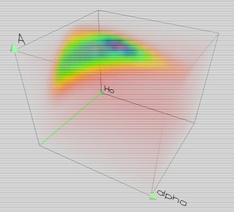
An ideal calculation to compute the $n$-dimensional integrals would include an infinite number of samples of parameter space points with infinite volume, but in practical estimations we are limited to choose a finite region of the parameter space (such that outside it the probabilities are almost null) and a finite number of samples. With this criteria, we have chosen $-1<\alpha\leqslant 7$ with resolution from $0.2$ to $0.5$. The lower resolution of $0.5$ is employed in the regions where the PDF changes slowly with respect to $\alpha$, which is interpolated to generate a higher resolution of $0.2$ for two and one-dimensional PDFs. Analogously, $55\leqslant H_{0}\leqslant 70$ with resolution of $1$, $0\leqslant\Omega_{m0}\leqslant 1$ with resolution of $0.05$, $0\leqslant\Omega_{c0}\leqslant 3.4$ with resolution of $0.17$ and $0\leqslant\bar{A}\leqslant 1$ with resolution of $0.05$. So there is a $5$-dimensional discrete space of $23\times 16\times 21\times 21\times 21$ points (total of $3,408,048$ points whose PDF values were calculated) as well as lower dimensional discrete spaces (fixing $\Omega_{m0}$, etc.), and the continuous PDFs in three, two and one-dimensional spaces are obtained by marginalizing interpolated functions built from the discrete points. We obviously discard the parameter space regions where the PDFs are not real numbers, as well as $t_{0}$ is not a positive real number.

Figure 1 illustrates the $3$-dimensional PDF of $(\alpha,H_{0},\bar{A})$, using a $3D$ density plot composed by voxels (volume elements) with transparency and colour attributes, specific to the $3$ free parameter case of the generalized Chaplygin gas model with $k=0$ and $\Omega_{m0}=0.04$ (the other five cases with $3$, $4$ and $5$ free parameters have similar $3D$ shapes). It is clearly visible the non-Gaussian behaviour of the $3$-dimensional PDF, with the orange and green $3D$ credible surfaces sharpening as $\alpha$ increases. Table 1 tells us that the maximum is located at $(\alpha,H_{0},\bar{A})=(27.0,62.7,1-5.5\times 10^{-9})$ but it is located at a very narrow region ($H_{0}$ is extremely peaked and $1-1\times 10^{-8}<\bar{A}<1$ with non-negligible PDF) therefore it would be invisible even if the graphics had the range $-1<\alpha\leqslant 28$ (because the needed resolution in the $\bar{A}$ axis would require approximately $10^{8}$ voxels in this dimension and only one voxel would be opaque and violet among them). Instead, in figure 1 we see a opaque violet region indicating a maximum near $(\alpha,H_{0},\bar{A})=(3.0,62,0.95)$ because there is non-negligible volume with high PDF values. The conclusion is simple: as $\alpha$ increases the high PDF regions narrow in width until becoming invisible, like the blue, green and yellow credible surfaces (corresponding to constant PDF levels) do in sequence as shown by figure 1.

The above behaviour is important to understand the results of the marginalization processes. For example, when the marginalization is applied to figure 1, i.e, resulting the bottom-right plot of figures 2. The integration of $p(\alpha,H_{0},\bar{A}\mid\mu_{0})$ over the $H_{0}$ parameter space yields $p(\alpha,\bar{A}\mid\mu_{0})$, the PDF maximum moves to lower values of $\alpha$, $(\alpha,\bar{A})=(2.75,0.95)$, because the high PDF regions for higher values of $\alpha$ have a small width with respect to $H_{0}$ and weight less than larger regions due to the integration over $H_{0}$. Taking the marginalization process even further, i.e., marginalizing $p(\alpha,\bar{A}\mid\mu_{0})$ over the $\bar{A}$ space to produce $p(\alpha\mid\mu_{0})$ illustrated by the bottom-right plot in figure 3, the PDF maximum is once again at lower $\alpha$, $\alpha=-0.30$, because the high PDF regions for higher values of $\alpha$ have a small width now with respect to $\bar{A}$ and weight less than larger regions due to the integration over $\bar{A}$.

	GCGM	GCGM :	GCGM :	GCGM :	GCGM : $k=0$,	GCGM : $k=0$,
		$k=0$	$\Omega_{m0}=0$	$\Omega_{m0}=0.04$	$\Omega_{m0}=0$	$\Omega_{m0}=0.04$
$\alpha$	$-0.85_{-0.15}^{+6.01}$	$-1.00_{-0.00}^{+6.48}$	$-0.51_{-0.49}^{+6.39}$	$-0.54_{-0.46}^{+6.04}$	$0.14_{-1.14}^{+4.85}$	$-0.30_{-0.70}^{+4.99}$
$H_{0}$	$62.0_{-3.4}^{+3.3}$	$61.3_{-2.8}^{+2.9}$	$61.6_{-3.4}^{+3.4}$	$61.8_{-3.5}^{+3.3}$	$61.9_{-2.9}^{+2.7}$	$61.8_{-2.8}^{+2.7}$
$\Omega_{k0}$	$-1.26_{-1.42}^{+1.32}$	$0$	$0.21_{-1.68}^{+0.79}$	$0.08_{-1.61}^{+0.88}$	$0$	$0$
$\Omega_{m0}$	$0.00_{-0.00}^{+0.86}$	$0.00_{-0.00}^{+0.36}$	$0$	$0.04$	$0$	$0.04$
$\Omega_{c0}$	$1.39_{-1.25}^{+1.21}$	$1.00_{-0.36}^{+0.0}$	$0.79_{-0.79}^{+1.68}$	$0.88_{-0.88}^{+1.61}$	$1$	$0.96$
$\bar{A}$	$1.00_{-0.39}^{+0.00}$	$1.00_{-0.34}^{+0.00}$	$0.94_{-0.46}^{+0.06}$	$0.95_{-0.43}^{+0.05}$	$0.94_{-0.35}^{+0.06}$	$0.94_{-0.33}^{+0.06}$
$t_{0}$	$15.3_{-3.2}^{+4.2}$	$14.9_{-2.2}^{+4.8}$	$14.3_{-2.4}^{+7.1}$	$14.2_{-2.0}^{+6.6}$	$14.2_{-1.8}^{+6.9}$	$14.2_{-1.7}^{+7.5}$
$q_{0}$	$-0.80_{-0.62}^{+0.86}$	$-0.59_{-0.37}^{+0.31}$	$-0.67_{-0.86}^{+0.84}$	$-0.61_{-0.93}^{+0.78}$	$-0.80_{-0.18}^{+0.43}$	$-0.89_{-0.10}^{+0.52}$
$a_{i}$	$0.67_{-0.37}^{+0.25}$	$0.57_{-0.25}^{+0.33}$	$0.77_{-0.77}^{+0.12}$	$0.77_{-0.54}^{+0.16}$	$0.75_{-0.64}^{+0.14}$	$0.74_{-0.49}^{+0.13}$
$p(\alpha>0)$	$0.92\,\sigma$	$1.05\,\sigma$	$1.18\,\sigma$	$1.12\,\sigma$	$1.25\,\sigma$	$1.18\,\sigma$
$p(\Omega_{k0}<0)$	$2.20\,\sigma$	$-$	$0.71\,\sigma$	$0.80\,\sigma$	$-$	$-$
$p(q_{0}<0)$	$2.21\,\sigma$	$3.31\,\sigma$	$1.66\,\sigma$	$1.75\,\sigma$	$3.65\,\sigma$	$3.72\,\sigma$
$p(a_{i}<1)$	$2.22\,\sigma$	$3.35\,\sigma$	$1.66\,\sigma$	$1.75\,\sigma$	$3.77\,\sigma$	$3.71\,\sigma$
$p(\dot{a}>0)$	$5.83\,\sigma$	$\infty\,\sigma$	$5.88\,\sigma$	$5.92\,\sigma$	$\infty\,\sigma$	$\infty\,\sigma$

Table 2: The estimated parameters for the generalized Chaplygin gas model (GCGM) and some specific cases of spatial section and matter content. We use the Bayesian analysis to obtain the peak of the one-dimensional marginal probability and the $2\,\sigma$ credible region for each parameter. $H_{0}$ is given in $km/M\!pc.s$, $\bar{A}$ in units of $c$, $t_{0}$ in $Gy$ and $a_{i}$ in units of $a_{0}$.

Table 2 is very comprehensive and resumes our results, listing all the Bayesian parameter estimations for six different cases of spatial section and matter content within the context of generalized Chaplygin gas model. The following sub-sections will analyse in detail this table and accompanying figures. More emphasis is spent into the analyses of the generalized Chaplygin gas parameter $\alpha$, because it is the subject of constant debate.

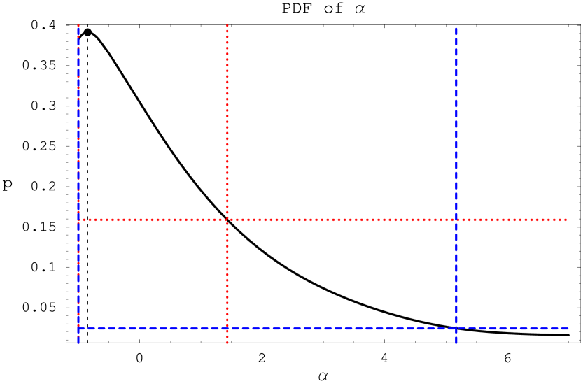
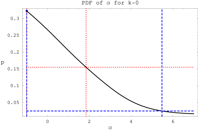
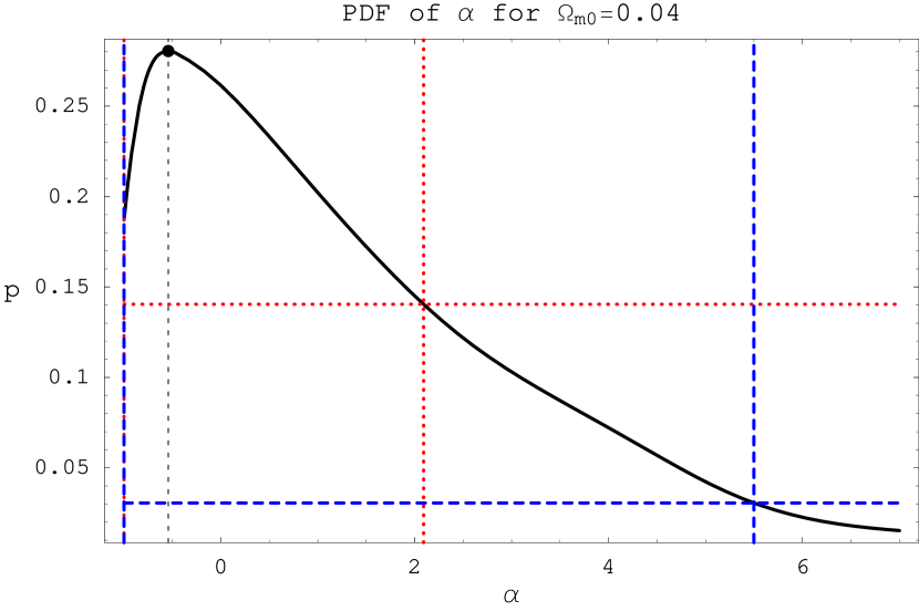
In figures 3, 4 and 6, the one-dimensional PDF shapes are matched against half-Gaussians to estimate the probabilities outside the left and right edges, in this way increasing the precision of the parameter estimations without excessively enlarging the parameter space.

4.1 $\alpha$ – the generalized Chaplygin gas parameter

The parameter estimation of $\alpha$ is strongly related to the $\bar{A}$ parameter, i.e., the joint PDFs for the parameter space of $(\alpha,\bar{A})$ do not have a Gaussian shape, so the marginalization process changes the peak values and credible regions. Table 2, figures 2 and 3 are carefully analysed below with respect to $\alpha$. In brief, the estimations for $\alpha$ are quite spread (i.e., they have large credible regions) and they differ a lot depending on if two or one-dimensional parameter space is used.

Figure 2: The graphics of the joint PDF as function of $(\alpha,\bar{A})$ for the generalized Chaplygin gas model. The joint PDF peak is shown by the large dot, the credible regions of $1\,\sigma$ ($68,27\%$) by the red dotted line, the $2\,\sigma$ ($95,45\%$) in blue dashed line and the $3\,\sigma$ ($99,73\%$) in green dashed-dotted line. The cases for $\Omega_{m0}=0$ are not shown here because they are similar to the ones with $\Omega_{m0}=0.04$.

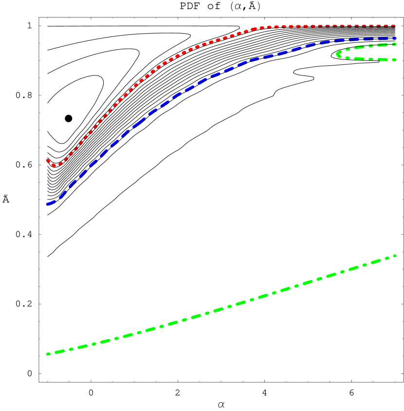
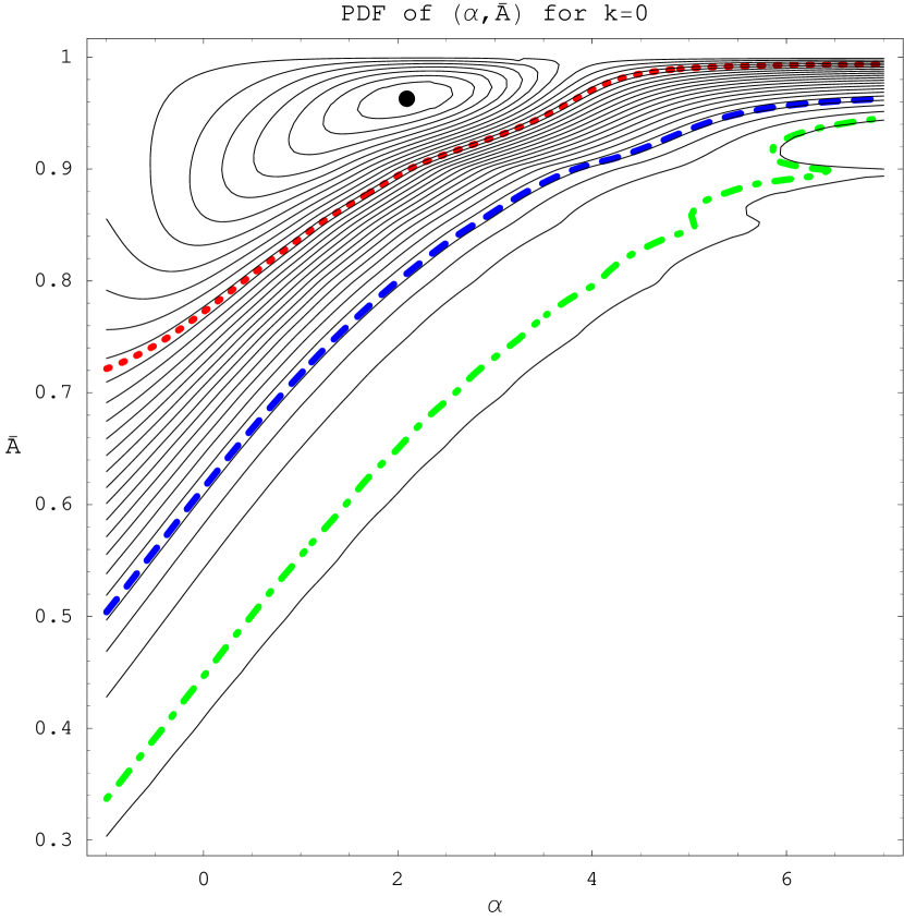
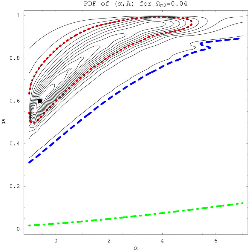
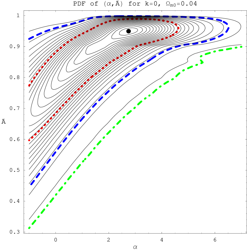
4.1.1 Generalized Chaplygin gas model with $5$ free parameters

In figures 2, the GCGM with $5$ free parameters has a joint PDF peak of $0.948$ at $(\alpha,\bar{A})=(-0.52,0.73)$ with $1\,\sigma$ ($68,27\,\%$), $2\,\sigma$ ($95,45\,\%$) and $3\sigma$ ($99,73\,\%$) credible region contours with PDF values of $0.717$, $0.123$ and $0.002$, respectively. The two-dimensional credible regions are not Gaussian-shaped, and their extremes give the estimations $(\alpha,\bar{A})=(-0.52_{-0.48}^{>+7.52},0.73_{-0.13}^{+0.27})$ at $1\,\sigma$, $(\alpha,\bar{A})=(-0.52_{-0.48}^{>+7.52},0.73_{-0.24}^{+0.27})$ at $2\,\sigma$, and $(\alpha,\bar{A})=(-0.52_{-0.48}^{>+7.52},0.73_{-0.67}^{+0.27})$ at $3\,\sigma$ confidence levels. The symbol ($>$) in the upper credible value for $\alpha$ is due to the fact that the graphics is limited to $-1<\alpha\leqslant 7$.

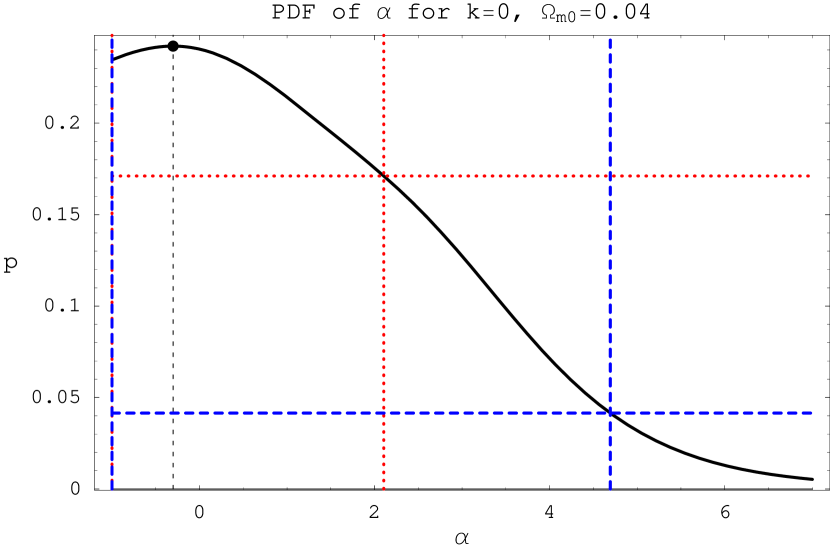
The marginalization (integration) of $p(\alpha,\bar{A}\mid\mu_{0})$ over the $\bar{A}$ space yields $p(\alpha\mid\mu_{0})$, shown in figure 3, where the credible intervals are $\alpha=-0.85_{-0.15}^{+2.28}$ at $1\,\sigma$ and $\alpha=-0.85_{-0.15}^{+6.01}$ at $2\,\sigma$ (the $3\,\sigma$ PDF level cannot be seen with $\alpha\leqslant 7$). The PDF peak of $0.383$ at $\alpha=-0.85$ is greater than the PDF value of $0.195$ for $\alpha=1$ (ordinary Chaplygin gas model), so the region with PDF greater than $0.195$ has a CDF of $0.607$, i.e., we can say that $\alpha=1$ is ruled out at a $60.7\,\%$ ($0.85\,\sigma$) confidence level (or it is preferred at $39.3\,\%$). Table 2 shows that positive values of $\alpha$ are more likely at a $64.1\,\%$ ($0.92\,\sigma$) confidence level.

4.1.2 GCGM with $4$ free parameters and $k=0$

The $4$-parameter case with $k=0$ has a joint PDF peak of $1.165$ at $(\alpha,\bar{A})=(2.09,0.96)$ with $1\,\sigma$, $2\,\sigma$ and $3\sigma$ credible region contour levels of $0.695$, $0.141$ and $0.007$, respectively. The two-dimensional credible regions give the estimations $(\alpha,\bar{A})=(2.09_{-3.09}^{>+4.91},0.96_{-0.24}^{+0.04})$ at $1\,\sigma$, $(\alpha,\bar{A})=(2.09_{-3.09}^{>+4.91},0.96_{-0.44}^{+0.04})$ at $2\,\sigma$, and $(\alpha,\bar{A})=(2.09_{-3.09}^{>+4.91},0.96_{-0.62}^{+0.04})$ at $3\,\sigma$ confidence levels.

The estimation based on $p(\alpha\mid\mu_{0})$ yields $\alpha=-1.00_{-0.00}^{+2.84}$ at $1\,\sigma$ and $\alpha=-1.00_{-0.00}^{+6.48}$ at $2\,\sigma$ confidence levels. The PDF peak of $0.323$ at $\alpha=-1.00$ is greater than the PDF value of $0.205$ for $\alpha=1$ such that $\alpha=1$ is ruled out at a $53.1\,\%$ ($0.72\,\sigma$) confidence level. Positive values of $\alpha$ are preferred at a $70.5\,\%$ ($1.05\,\sigma$) confidence level.

Figure 3: The PDF of $\alpha$ for the generalized Chaplygin gas model. The solid lines are the PDF, the $1\sigma$ ($68.27\%$) regions are delimited by red dotted lines and the $2\sigma$ ($95.45\%$) credible regions are given by blue dashed lines. The cases for $\Omega_{m0}=0$ are not shown here because they are similar to the ones with $\Omega_{m0}=0.04$.

4.1.3 GCGM with $4$ free parameters and $\Omega_{m0}=0$

The joint PDF has a peak value of $1.239$ at $(\alpha,\bar{A})=(-0.51,0.60)$ with $1\,\sigma$, $2\,\sigma$ and $3\sigma$ credible region contour levels of $0.378$, $0.017$ and $0.007$, respectively. These levels indicate that the joint two-dimensional PDF is strongly peaked. The two-dimensional credible regions give the estimations $(\alpha,\bar{A})=(-0.51_{-0.45}^{+4.97},0.60_{-0.12}^{+0.40})$ at $1\,\sigma$, $(\alpha,\bar{A})=(-0.51_{-0.49}^{>+7.51},0.60_{-0.35}^{+0.40})$ at $2\,\sigma$, and $(\alpha,\bar{A})=(-0.51_{-0.49}^{>+7.51},0.60_{-0.58}^{+0.40})$ at $3\,\sigma$ confidence levels.

The estimations based on one-dimensional PDF yield the same peak value (due to the highly peaked joint PDF), with $\alpha=-0.51_{-0.46}^{+2.86}$ at $1\,\sigma$ and $\alpha=-0.51_{-0.49}^{+6.39}$ at $2\,\sigma$ confidence levels. The PDF peak of $0.263$ at $\alpha=-0.51$ is greater than the PDF value of $0.200$ for $\alpha=1$, and we can say that $\alpha=1$ is preferred at a $55.9\,\%$ ($0.77\,\sigma$) confidence level. Positive values of $\alpha$ are preferred at a $76.2\,\%$ ($1.18\,\sigma$) confidence level.

4.1.4 GCGM with $4$ free parameters and $\Omega_{m0}=0.04$

The joint PDF has a peak value of $1.257$ at $(\alpha,\bar{A})=(-0.56,0.60)$ with $1\,\sigma$, $2\,\sigma$ and $3\sigma$ credible region contour levels of $0.428$, $0.020$ and $0.005$, respectively, which show a highly peaked behaviour. The two-dimensional credible regions give the estimations $(\alpha,\bar{A})=(-0.56_{-0.44}^{+5.69},0.60_{-0.10}^{+0.40})$ at $1\,\sigma$, $(\alpha,\bar{A})=(-0.56_{-0.44}^{>+7.56},0.60_{-0.29}^{+0.40})$ at $2\,\sigma$, and $(\alpha,\bar{A})=(-0.56_{-0.44}^{>+7.56},0.60_{-0.58}^{+0.40})$ at $3\,\sigma$ confidence levels.

The estimations based on one-dimensional PDF give $\alpha=-0.54_{-0.46}^{+2.63}$ at $1\,\sigma$ and $\alpha=-0.54_{-0.46}^{+6.04}$ at $2\,\sigma$ confidence levels. The PDF peak of $0.280$ at $\alpha=-0.54$ is greater than the PDF value of $0.202$ for $\alpha=1$, and we can say that $\alpha=1$ is preferred at a $50.9\,\%$ ($0.69\,\sigma$) confidence level. Positive values of $\alpha$ are preferred at a $73.6\,\%$ ($1.12\,\sigma$) confidence level.

4.1.5 GCGM with $3$ free parameters and $k=0$, $\Omega_{m0}=0$

The joint PDF has a peak value of $1.336$ at $(\alpha,\bar{A})=(3.11,0.95)$ with $1\,\sigma$, $2\,\sigma$ and $3\sigma$ credible region contour levels of $0.583$, $0.115$ and $0.007$, respectively. The two-dimensional credible regions give the estimations $(\alpha,\bar{A})=(3.11_{-4.11}^{+1.86},0.95_{-0.38}^{+0.04})$ at $1\,\sigma$, $(\alpha,\bar{A})=(3.11_{-4.11}^{+3.72},0.95_{-0.52}^{+0.05})$ at $2\,\sigma$, and $(\alpha,\bar{A})=(3.11_{-4.11}^{>+3.89},0.95_{-0.65}^{+0.05})$ at $3\,\sigma$ confidence levels.

The estimations based on one-dimensional PDF give $\alpha=0.14_{-1.14}^{+2.22}$ at $1\,\sigma$ and $\alpha=0.14_{-1.14}^{+4.85}$ at $2\,\sigma$ confidence levels. The PDF peak of $0.222$ at $\alpha=0.14$ is greater than the PDF value of $0.208$ for $\alpha=1$, and we can say that $\alpha=1$ is preferred at a $63.2\,\%$ ($0.90\,\sigma$) confidence level. Positive values of $\alpha$ are preferred at a $78.8\,\%$ ($1.25\,\sigma$) confidence level.

4.1.6 GCGM with $3$ free parameters and $k=0$, $\Omega_{m0}=0.04$

The joint PDF has a peak value of $1.367$ at $(\alpha,\bar{A})=(2.75,0.95)$ with $1\,\sigma$, $2\,\sigma$ and $3\sigma$ credible region contour levels of $0.595$, $0.113$ and $0.007$, respectively. The two-dimensional credible regions give the estimations $(\alpha,\bar{A})=(2.75_{-4.75}^{+1.88},0.95_{-0.35}^{+0.04})$ at $1\,\sigma$, $(\alpha,\bar{A})=(2.75_{-4.75}^{+3.77},0.95_{-0.50}^{+0.05})$ at $2\,\sigma$, and $(\alpha,\bar{A})=(2.75_{-4.75}^{>+4.25},0.95_{-0.63}^{+0.05})$ at $3\,\sigma$ confidence levels.

The estimations based on one-dimensional PDF give $\alpha=-0.30_{-0.70}^{+2.41}$ at $1\,\sigma$ and $\alpha=-0.30_{-0.70}^{+4.99}$ at $2\,\sigma$ confidence levels. The PDF peak of $0.242$ at $\alpha=-0.30$ is greater than the PDF value of $0.214$ for $\alpha=1$, and we can say that $\alpha=1$ is preferred at a $53.1\,\%$ ($0.72\,\sigma$) confidence level. Positive values of $\alpha$ are preferred at a $76.0\,\%$ ($1.18\,\sigma$) confidence level.

The non-Gaussian shape of the credible region contours in the $(\alpha,\bar{A})$ two-dimensional parameter space is the culprit of this difference for the estimations of $\alpha$, so it is crucial to emphasize how the $\alpha$ parameter is estimated : from a joint two-dimensional PDF or an one-dimensional PDF (after marginalization of the joint two-dimension PDF). The most robust parameter estimation is based on the one-dimensional PDF, therefore giving small importance to regions in the joint two-dimensions which have a small joint PDF volume (CDF). Comparing the estimations, the ones based on two-dimensional parameter space always give larger values for $\alpha$, after marginalization the PDF is peaked at lower values of $\alpha$.

We also expect that a large sample of SNe Ia will narrow the credible regions of $\alpha$, so the issue of a ordinary Chaplygin gas model (CGM) being preferred or ruled out will be probably better addressed.

4.2 The parameter $\bar{A}$

The generalized Chaplygin gas model (GCGM) estimations for $\bar{A}$ are given by table 2, which if compared with the results of the CGM (table $5$ of ref. [17]) clearly indicate that the PDF peak is closer to $\bar{A}=1$ and the dispersion is increased when the GCGM is considered. This behaviour is due to the shape of the joint PDF in the parameter space $(\alpha,\bar{A})$, figures 2 explicitly show that as $\alpha$ increases there is a narrower region of high PDF values closer to higher values of $\bar{A}$.

But the estimations for $\bar{A}$ shown in table 2 and figures 4 have to be interpreted. They do not indicate that the $\Lambda CDM$ limit ($\bar{A}=1$) is favoured because the resolution for the $\bar{A}$ sampling is $0.05$, i.e, a PDF peak at $\bar{A}=1.00$ means the peak happens for $0.95<\bar{A}\leqslant 1$ indeed. Therefore, in figures 4, the graphics for the PDF of $\bar{A}$ which are peaked at $\bar{A}=1$ have the shape of the graphics for the case $\Omega_{m0}=0.04$, with the PDF peak closer to $\bar{A}=1$. See ref. [17] for a detailed comparison between the CGM and $\Lambda CDM$ cases.

Figure 4: The one-dimensional PDF of $\bar{A}$ for the generalized Chaplygin gas model. The solid lines are the PDF, the $1\sigma$ ($68.27\%$) regions are delimited by red dotted lines, the $2\sigma$ ($95.45\%$) credible regions are given by blue dashed lines and the $3\sigma$ ($99.73\%$) regions are delimited by green dashed-dotted lines. The cases for $\Omega_{m0}=0$ are not shown here because they are similar to the ones with $\Omega_{m0}=0.04$.

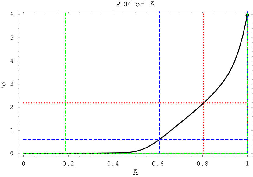
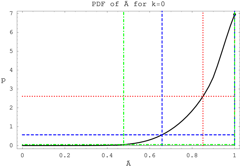
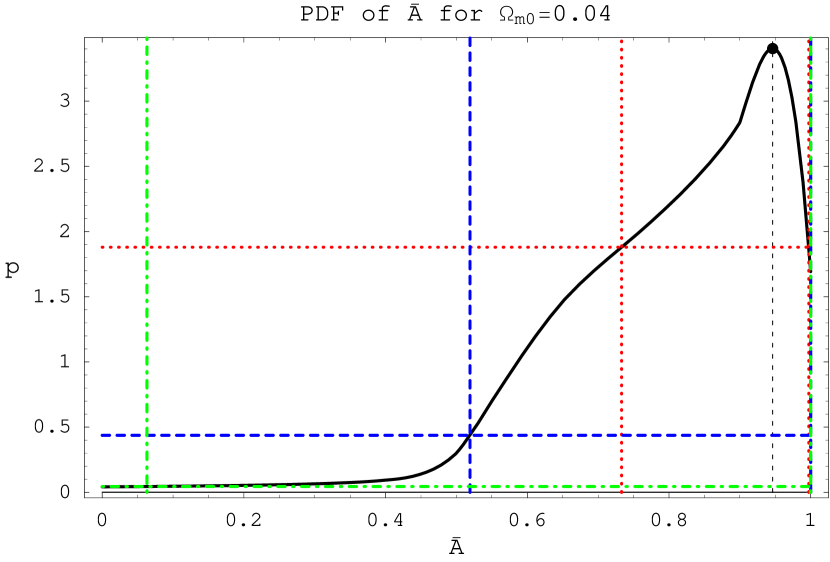
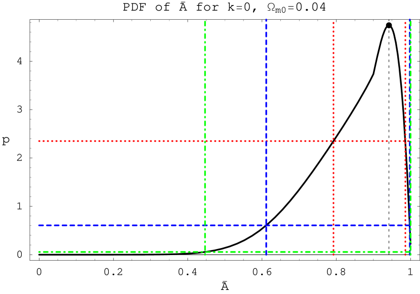
The analyses of $\alpha$ presented above have considered the joint PDFs for the two-dimensional parameter space of $(\alpha,\bar{A})$, and the extremes of the credible regions have given estimations for $(\alpha,\bar{A})$ at $1\,\sigma$, $2\,\sigma$, and $3\,\sigma$ confidence levels. These estimations for $\bar{A}$ are almost always different from the estimations based on the one-dimensional PDF of $\bar{A}$, obtained by marginalizing $p(\alpha,\bar{A}\mid\mu_{0})$ over the $\alpha$ space. We stress again that the most robust estimations are based on the one-dimensional PDFs. The general behaviour of table 2 is that the PDF peak is at $0.95<\bar{A}\leqslant 1$ and the $2\,\sigma$ credible interval begins at $\bar{A}\simeq 0.5$ and finishes at $\bar{A}\simeq 1$.

4.3 The Hubble parameter $H_{0}$

The parameter estimation of $H_{0}$ shown in table 2 is almost the same for all cases, around $62\ km/M\!pc.s$ with a narrow credible region of $\pm 3\ km/M\!\!pc.s$. This estimation, like the one for the CGM in table $5$ of ref. [17], is compatible with other SNe Ia analyses.

4.4 The curvature density parameter $\Omega_{k0}$

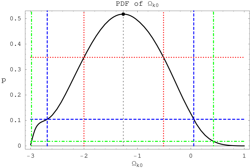
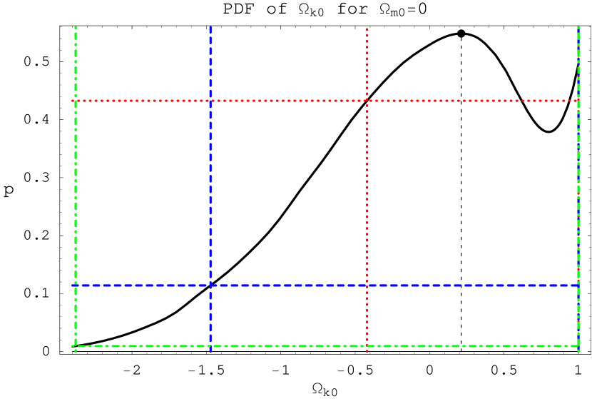
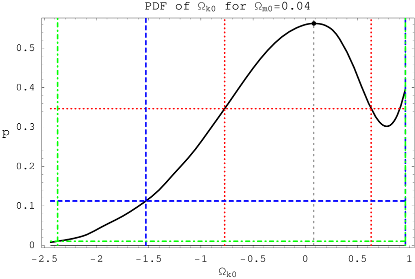
Table 2 and figure 6 show that the curvature density parameter $\Omega_{k0}$ estimation for the GCGM is almost like for the CGM of ref. [17], i.e., it also strongly depends on the cold dark matter content of the GCGM.

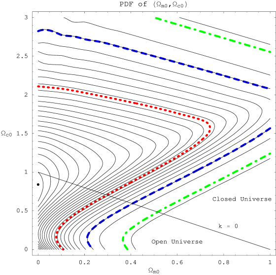
In the $5$-parameter case a closed Universe ($\Omega_{k0}<0$) is preferred at $97.19\,\%$ ($2.20\,\sigma$) and a spatially flat Universe is ruled out at $93.44\,\%$ ($1.84\,\sigma$) confidence level, i.e., the PDF of $\Omega_{k0}=0$ is smaller than the PDF of $-2.57<\Omega_{k0}<0$ and this region has a CDF of $93.44\,\%$ ($1.84\,\sigma$). We can also see the figure 5 that the integral of the joint PDF over the upper region gives the same high likelihood of a closed Universe, although the joint PDF peak is located in the open Universe region.

Figure 5: The graphics of the joint PDF as function of $(\Omega_{m0},\Omega_{c0})$ for the generalized Chaplygin gas model, where $p(\Omega_{m0},\Omega_{c0})$ is a integral of $p(\alpha,H_{0},\Omega_{m0},\Omega_{c0},\bar{A})$ over the $(\alpha,H_{0},\bar{A})$ parameter space. It shows a different shape for the confidence regions with respect to the $\Lambda CDM$ but similar to the CGM of ref. [17]. The joint PDF peak has the value $1.39$ for $(\Omega_{m0},\Omega_{c0})=(0.00,0.81)$ (shown by the large dot), the credible regions of $1\,\sigma$ ($68,27\%$, shown in red dotted line), $2\,\sigma$ ($95,45\%$, in blue dashed line) and $3\,\sigma$ ($99,73\%$, in green dashed-dotted line) have PDF levels of $0.50$, $0.13$ and $0.02$, respectively. As $\Omega_{k0}+\Omega_{m0}+\Omega_{c0}=1$, the probability for a spatially flat Universe is on the line $\Omega_{m0}+\Omega_{c0}=1$, above it we have the region for a closed Universe ($k>0$, $\Omega_{k0}<0$), and below, the region for an open Universe ($k<0$, $\Omega_{k0}>0$).

But assuming the hypothesis that $\Omega_{m0}=0.04$, a $4$-parameter case, the behaviour is opposite, a closed Universe ($\Omega_{k0}<0$) is preferred at $57.75\,\%$ ($0.80\,\sigma$) and a spatially flat Universe is preferred at $90.32\,\%$ ($1.66\,\sigma$) confidence level, i.e., the PDF of $\Omega_{k0}=0$ is smaller than the PDF of $0<\Omega_{k0}<0.17$ and this region has a small CDF of $9.68\,\%$. Therefore, if we impose a low value for $\Omega_{m0}$ then the spatially flat Universe is favoured.

Figure 6: The one-dimensional PDF of $\Omega_{k0}$, $\Omega_{m0}$ and $\Omega_{c0}$ for the generalized Chaplygin gas model. The solid lines are the PDF, the $1\sigma$ ($68.27\%$) regions are delimited by red dotted lines, the $2\sigma$ ($95.45\%$) credible regions are given by blue dashed lines and the $3\sigma$ ($99.73\%$) regions are delimited by green dashed-dotted lines. As $\Omega_{c0}=1-\Omega_{k0}-\Omega_{k0}$, for $\Omega_{m0}=0$ we have $\Omega_{c0}=1-\Omega_{k0}$, for $\Omega_{m0}=0.04$ then $\Omega_{c0}=0.96-\Omega_{k0}$ and for $\Omega_{k0}=0$ we also have $\Omega_{c0}=1-\Omega_{m0}$.

4.5 The cold dark matter density parameter $\Omega_{m0}$

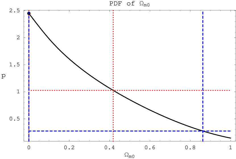
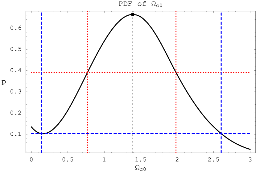
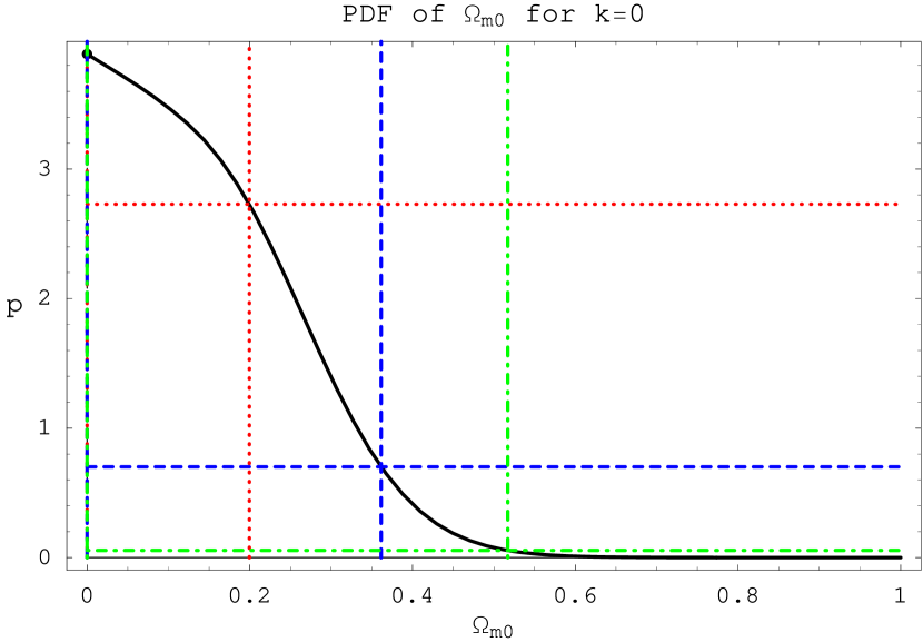
The generalized Chaplygin gas model favours small values of $\Omega_{m0}$ like the ordinary CGM, see table 2 and table $5$ of ref. [17]. The graphics for $\Omega_{m0}$ in figure 6, for the $5$-parameter case and $4$-parameter case with $k=0$, shows a estimation for $\Omega_{m0}$ peaked at $0$ at a high level of confidence, with $\Omega_{m0}<0.42$ (for the $5$-parameter case) and $\Omega_{m0}<0.20$ (for $4$-parameter case with $k=0$) at $1\,\sigma$ ($68.27\%$) confidence level. As $\Omega_{m0}$ was sampled with bin size $0.05$, then the peaks can be somewhere between $0.00$ and $0.05$.

The joint PDF for the parameter space of $(\Omega_{m0},\Omega_{c0})$, i.e, $p(\Omega_{m0},\Omega_{c0}\mid\mu_{0})$, is shown in figure 5. The PDF peak is now located at $(\Omega_{m0},\Omega_{c0})=(0.0,0.81)$, with the same the central value of $\Omega_{m0}$ after Bayesian marginalization. But, in this two-parameter space with simultaneously values of $(\Omega_{m0},\Omega_{\Lambda})$, the credible regions would be given by $(\Omega_{m0},\Omega_{c0})=(0.0_{-0.00}^{+0.74},0.81_{-0.81}^{+1.31})$ at $1\,\sigma$ ($68,27\%$) and $(\Omega_{m0},\Omega_{c0})=(0.0_{-0.00}^{+1.14},0.81_{-0.81}^{+2.05})$ at $2\,\sigma$ ($95,45\%$) confidence levels. Of course, the integral (marginalization) of $p(\Omega_{m0},\Omega_{c0}\mid\mu_{0})$ over the $\Omega_{c0}$ space yields $p(\Omega_{m0}\mid\mu_{0})$, shown in figure 6. The conclusion is that the marginalization decreases the confidence regions, even if it does not change the peak value of probability.

4.6 The generalized Chaplygin gas density parameter $\Omega_{c0}$

The generalized Chaplygin gas density parameter $\Omega_{c0}$ estimation (table 2) is like the estimation in the case of CGM shown by table $5$ of ref. [17], and is quite spread, i.e., it has a large credible region, for example $\Omega_{c0}=1.39_{-1.25}^{+1.21}$ in the case of $5$-parameter space. Figure 6 show the PDF of $\Omega_{c0}$ for the $5$-parameter space (showing $\Omega_{c0}=1.39_{-0.62}^{+0.59}$ at $1\,\sigma$ confidence level)  and the $4$-parameter space with $k=0$ (when $\Omega_{c0}=1-\Omega_{m0}$).

As discussed above for the GCGM, the joint PDF for the parameter space of $(\Omega_{m0},\Omega_{c0})$ in figure 5 shows  that the credible regions would be given by $(\Omega_{m0},\Omega_{c0})=(0.0_{-0.00}^{+0.74},0.81_{-0.81}^{+1.31})$ at $1\,\sigma$ ($68,27\%$) and $(\Omega_{m0},\Omega_{c0})=(0.0_{-0.00}^{+1.14},0.81_{-0.81}^{+2.05})$ at $2\,\sigma$ ($95,45\%$) confidence level. So, the marginalization of $p(\Omega_{m0},\Omega_{c0}\mid\mu_{0})$ over the $\Omega_{m0}$ space gives $p(\Omega_{c0}\mid\mu_{0})$, yielding a different peak value as well as different (narrower) confidence regions.

4.7 The present age $t_{0}$ of the Universe

The estimates for the dynamical age of the Universe today, $t_{0}$, given in table 2, show that the generalized Chaplygin gas model increases the $2\,\sigma$ credible regions (e.g., $t_{0}=15.3_{-3.2}^{+4.2}\,Gy$), when compared to the estimations of the CGM in table $5$ of ref. [17] (e.g., $t_{0}=14.2_{-1.5}^{+2.8}\,Gy$). The peak values of $t_{0}$ range between $14.2\,Gy$ to $15.3\,Gy$, while the CGM features $t_{0}$ peaked between $13.1\,Gy$ to $14.8\,Gy$. We expect that a large sample of SNe Ia will narrow the credible regions and allow, by means of independent estimations of $t_{0}$ from different observations (globular agglomerates, etc), to verify which cosmological model is preferred : GCGM, CGM and $\Lambda$CDM.

Table 1 shows the $t_{0}$ for the best-fitting parameters without any marginalization (i.e., the $n$-parameter model has its $n$ parameters taken simultaneously yielding a minimum $\chi^{2}$) : the $t_{0}$ ranges from $14.0Gy$ to $14.4\,Gy$, well inside the estimated credible regions for $t_{0}$.

4.8 The deceleration parameter $q_{0}$ of the Universe

All the estimations based on the generalized Chaplygin gas model (table 2) suggest an accelerating Universe today, i.e., $q_{0}<0$, with a high confidence level ranging from $1.66\,\sigma$ ($90.24\,\%$) to $3.72\,\sigma$ ($99.98\,\%$), depending on the curvature and cold dark matter densities of the Universe. The peak values of $q_{0}$ range between $-0.89$ to $-0.59$. The data of CGM in table $5$ of ref. [17] show a similar behaviour.

Although the $q_{0}$ values of Table 1, from $-1.00$ to $-0.80$, are inside the estimated credible regions for $q_{0}$, the estimated peak values of $q_{0}$ differs from the $q_{0}$ for the best-fitting parameters.

4.9 The inflexion point $a_{i}$ for the scale factor

We have also estimated the value of the scale factor that shows the beginning of the recent accelerating phase of the Universe. Table 2 shows that the most probable value for $a_{i}$ ranges between $0.57\,a_{0}$ to $0.77\,a_{0}$, where $a_{0}$ is the value of scale factor today, with usually an small upper credible region and a larger lower credible region.

The probability of $a_{i}<a_{0}$ is theoretically the same having an accelerating Universe today ($q_{0}<0$), and these independent probability calculations agree almost exactly as table 2 shows, indicating that the Bayesian probability analyses of this work are accurate and reliable for the given SNe Ia data.

We can obviously express the scale factor value $a_{i}$ in terms of redshift value $z_{i}$, $a_{i}/a_{0}=1/(1+z_{i})$ or $z_{i}=-1+(a_{0}/a_{i})$. For example, $a_{i}=0.67_{-0.37}^{+0.25}\,a_{0}$ corresponds to $z_{i}=0.49_{-0.41}^{+1.87}$. We expect that a large sample of SNe Ia with large redshift values will help improve this type of estimation of $z_{i}$ or equivalently $a_{i}$.

The $a_{i}$ values are almost equal in table 1 for the best-fitting parameters, between $0.756\,a_{0}$ and $0.792\,a_{0}$, and this range fits well inside the the estimated credible regions for $a_{i}$ of table 2.

4.10 The eternally expanding Universe

The probability of having a eternally expanding Universe, given here by demanding $\dot{a}>0$ during the future evolution of the Universe, is estimated to be exactly one or almost one (at almost a $6\,\sigma$ level), see table 2. The estimations for the CGM and $\Lambda$CDM cases (tables $4$ and $5$, ref. [17]) were miscalculated, they are also exactly one or almost one.

5 Conclusion

In this paper we investigated some constraints on the generalized Chaplygin gas model (GCGM) using type Ia supernovae data and Bayesian statistics. The model is built with the Chaplygin gas and a pressureless fluid as the matter content of the Universe, whose density parameters today are $\Omega_{c0}$ and $\Omega_{m0}$ respectively, such that the curvature term is $\Omega_{k0}=1-\Omega_{m0}-\Omega_{c0}$. The parameter $\bar{A}$ related to the sound velocity of the Chaplygin gas, the Hubble parameter $H_{0}$ and the $\alpha$ parameter are also independent free variables. We allowed the parameter $\alpha$ to vary between negative and large positive values. In principle, this could lead to instability problems at perturbative level ($\alpha$ negative), or superluminal sound velocity ($\alpha$ greater than one), but both potential problems can be resolved using a fundamental description for the GCG.

When the five independent parameters are free, the Bayesian estimation yields $\alpha=-0.86_{-0.15}^{+6.01}$, $H_{0}=62.0_{-1.42}^{+1.32}\,km/Mpc.s$, $\Omega_{k0}=-1.26_{-1.42}^{+1.32}$, $\Omega_{m0}=0.00_{-0.00}^{+0.86}$, $\Omega_{c0}=1.39_{-1.25}^{+1.21}$, $\bar{A}=1.00_{-0.39}^{+0.00}$, $t_{0}=15.3_{-3.2}^{+4.2}$, $q_{0}=-0.80_{-0.62}^{+0.86}$ and $a_{i}=0.67_{-0.37}^{+0.25}\,a_{0}$ where $t_{0}$ is the age of the Universe, $q_{0}$ is the value of the deceleration parameter today and $a_{i}$ is the value of the scale factor that marks the start of the recent accelerating phase of the Universe. We have also estimated the cosmological parameters fixing the pressureless matter (through the constraints of nucleosynthesis) or the curvature (imposing the flat condition), or even both. The estimations of the remaining free parameters do not change dramatically in each case, with some exceptions. For example, the prediction for the curvature parameter depends on whenever the pressureless matter is fixed or not : a spatially flat Universe is favoured only if $\Omega_{m0}$ is fixed at low values.

In particular, we verify that the $\alpha$ parameter is strongly related to the $\bar{A}$ parameter. In this manner, the best value of $\alpha$ have the peak values and the credible regions changed in function of the marginalization process used. The $\alpha$ estimations are very spread and differ a lot if one or two-dimensional parameter space is used. Many authors [18]–[25], prefer to estimate $\alpha$ and $\bar{A}$ simultaneously using two-dimensional credible regions and they do not marginalize the PDF to obtain the more statistically robust one-dimensional PDFs for $\alpha$ and $\bar{A}$, so any comparison should be taken carefully as the credible region estimations on two-dimensional parameter space are usually different from the one-dimensional estimations.

Here we take the marginalization approach to obtain one-dimensional PDFs, and one important point arises in this analysis : despite the dependency on the $\bar{A}$ parameter, the value $\alpha=1$, that represents the ordinary CGM, is not ruled out since this particular case is preferred at $39.3\%$ to $63.2\%$, depending on the spatial section and matter content.

We calculated the value of the scale factor when the dark energy starts to prevail, $a_{i}=0.67~{}a_{0}$, for the case of five free parameters. In general, the value for $a_{i}$ ranges between $0.57~{}a_{0}$ and $0.77~{}a_{0}$, where $a_{0}$ is the value of the scale factor today. This results are coherent with the suposition that the recent acceleration of the Universe could be started with the redshift parameter $z$ between $0$ and $1$ obtained by the type Ia supernovae data.

In the case of the ordinary matter parameter $\Omega_{m0}$ our analyses show that the preferred values are small, around zero. This situation is the same of the case of the ordinary Chaplygin gas. The result reinforces the idea of the Quartessence model [12, 14, 18], that unifies dark matter and dark energy into a single fluid, the Chaplygin gas. The predicted age of the Universe is well above the age of globular clusters. At same time, the deceleration parameter is consistent with the estimations from the WMAP data.

Further developments of the present work include the use of a large sample of type Ia supernovae. However, the sample of $26$ SNe Ia used here has an excellent quality with respect to the low values of $\chi_{\nu}^{2}$. Moreover, the dispersion of the parameter estimations obtained here has the same order of estimations using larger samples. In some cases our estimation are even less spread, as our preliminary investigation on larger SNe Ia indicates.

We also plan to apply the Bayesian analysis to the GCGM using large scale structures data (2dFRGS) and to the anisotropy of the cosmic microwave background. In this way, we may consistently cross the estimations of different observational data and constrain more sharply the predictions to each free parameter of the model.

Acknowledgments

We would like to thank Orfeu Bertolami, Ioav Waga and Martín Makler for many discussions about the generalized Chaplygin gas model. The authors are also grateful by the received financial support during this work, from CNPq (J. C. F. and S. V. B. G.) and FACITEC/PMV (R. C. Jr.).

References

- [1] V. Sahni, Dark Matter and Dark Energy, lectures presented at the Second Aegean Summer School on the Early Universe, Syros, Greece, September 2003, astro-ph/0403324;
- [2] J. Einasto and M. Einasto, Publ. Astron. Soc. Pac. 209, 360 (2000);
- [3] A. G. Riess et al., Astron. J. 116, 1009 (1998);
- [4] S. Permultter et al., Astrophys. J. 517, 565 (1998);
- [5] E. P. S. Shellard and R. A. Battye, Phys. Rept. 307, 227 (1998);
- [6] P. J. E. Peebles and Bharat Ratra, Rev. Mod. Phys. 75, 559 (2003);
- [7] R. R. Caldwell, R. Dave and P. Steinhardt, Phys. Rev. Lett. 80, 1582 (1998);
- [8] V. Sahni, Class. Quant. Grav. 19, 3435 (2002);
- [9] Ph. Brax and J. Martin, Phys. Lett. B468, 40 (1999);
- [10] C. Kolda and D. H. Lyth, Phys. Lett. B458, 197 (1999);
- [11] S. M. Carroll, Liv. Rev. Rel. 4, 1 (2001);
- [12] A. Yu. Kamenshchik, U. Moschella and V. Pasquier, Phys. Lett. B511, 265 (2001);
- [13] J.C. Fabris, S.V.B. Gonçalves and P.E. de Souza, Gen. Rel. Grav. 34, 53 (2002);
- [14] N. Bilić, G. B. Tupper and R. D. Viollier, Phys. Lett. B535, 17 (2002);
- [15] M. C. Bento, O. Bertolami and A. A. Sen, Phys. Rev. D66, 043507 (2002);
- [16] J. C. Fabris and J. Martin, Phys. Rev. D55, 5205 (1997);
- [17] R. Colistete Jr, J. C. Fabris, S. V. B. Gonçalves and P.E. de Souza, Int. J. Mod. Phys. D13, 669 (2004);
- [18] M. Makler, S. Q. de Oliveira and I. Waga, Phys. Lett. B555, 1 (2003);
- [19] P. P. Avelino, L. M. G. Beca, J. P. M. de Carvalho, C. J. A. P. Martins and P. Pinto. Phys. Rev. D67, 023511 (2003);
- [20] M. C. Bento, O. Bertolami and A. A. Sen, Gen. Rel. Grav. 35, 2063 (2003);
- [21] L. Amendola, F. Finelli, C. Burigana and D. Carturan, JCAP 0307, 005 (2003);
- [22] M. C. Bento, O. Bertolami and A. A. Sen, Phys. Lett. B575, 172 (2003);
- [23] J. S. Alcaniz and J. A. S. Lima, Measuring the Chaplygin gas equation of state from angular and luminosity distances, astro-ph/0308465;
- [24] M. Makler, S. Q. de Oliveira and I. Waga, Phys. Rev. D68, 123521 (2003);
- [25] O. Bertolami, A. A. Sen, S. Sen and P. T. Silva, Mon. Not. Roy. Astron. Soc. 353, 329 (2004);
- [26] M. Biesiada, W. Godlowski and M. Szydlowski, Generalized Chaplygin Gas Models tested with SNIa, astro-ph/0403305;
- [27] O. Bertolami, Challenges to the Generalized Chaplygin Gas Cosmology, based on talks presented at Oporto, Bilbao and Campos do Jordão, astro-ph/0403310;
- [28] M. C. Bento, O. Bertolami and A. A. Sen, The Revival of the Unified Dark Energy-Dark Matter Model ?, astro-ph/0407239;
- [29] N. Bilic, R. J. Lindebaum, G. B. Tupper and Raoul D. Viollier, The Chaplygin gas and the evolution of dark matter and dark energy in the Universe, astro-ph/0307214;
- [30] J.C. Fabris, S. V. B. Gonçalves and R. de Sá Ribeiro, Gen. Rel. Grav. 36, 211 (2004);
- [31] P. T. Silva and O. Bertolami, Astrophys. J. 599, 829 (2003);
- [32] J. V. Cunha, J. S. Alcaniz and J. A. S. Lima, Phys. Rev. D69, 083501 (2004);
- [33] J. S. Alcaniz, D. Jain and A. Dev, Phys. Rev. D67, 043514 (2003);
- [34] A. G. Riess et al., Astrophys. J. 607, 665 (2004);
- [35] J. L. Tonry et al, Astrophys. J. 594, 1 (2003);
- [36] B. J. Barris et al, Astrophys.J. 602, 571 (2004);
- [37] V. Gorini, A. Kamenshchik, U. Moschella and V. Pasquier, The Chaplygin gas as a model for dark energy, gr-qc/0403062;
- [38] L. P. Chimento, Phys. Rev. D69, 123517 (2004);
- [39] L. M. Krauss and B. Chaboyer, Nature 299, 65 (2003);
- [40] Y. Wang, Astrophys. J. 536, 531 (2000);
- [41] S. Nesseris and L. Perivolaropoulos, Phys. Rev. D70, 043531 (2004);
- [42] S. Wolfram, The Mathematica Book (Cambridge University Press), 1999.