SPhT-Saclay t04/110

Constraints on higher-dimensional gravity from the cosmic shear three-point correlation function

Abstract

With the developments of large galaxy surveys or cosmic shear surveys it is now possible to map the dark matter distribution at truly cosmological scales. Detailed examinations of the statistical properties of the dark matter distribution reveal the detail of the large-scale structure growth of the Universe. In particular it is shown here that the behavior of the density field bi-spectrum is sensitive to departure from normal gravity in a way which depends only weakly on the background evolution. The cosmic shear bispectrum appears to be particularly sensitive to changes in the Poisson equation: we show that the current cosmic shear data can already be used to infer constraints on the scale of a possible higher-dimensional gravity, above 2 $h^{-1}$Mpc.

Almost all cosmological observations point toward a coherent model in which there is a non-vanishing dark energy [1]. The existence of such a component is very puzzling from a high energy physics point of view and signals physics beyond the standard model in way we do not yet apprehend. The resolution of such an issue may lie either in the introduction of a new form of cosmic fluid - a dark energy - with a negative pressure that would correspond to two third of the actual energy density of the universe or maybe in a modification of the Einstein gravity equations at cosmological scales. The two scenarios have obviously to be distinguished [2]! The first route is usually taken in models evoking quintessence component. However it cannot excluded that a non-zero cosmological constant observation actually signals a modification of the Einstein law at cosmological scales. This idea is actually fuelled by recent developments in string theory phenomenologies. Indeed the introduction of branes in the context of superstring theories[3, 4], led to concepts of higher dimensional spacetimes. Usually it is assumed that the interaction gauge fields are localized on a 3–brane (i.e. a 3+1 dimension spacetime) whereas gravity propagates in all dimensions. In any of such string inspired models, one expects both the existence of Kaluza-Klein gravitons implying a non standard gravity on very small scales and light bosons, which can manifest as a new fundamental small scale force. It cannot be however excluded that gravity might be modified at large cosmological scale as well  [5, 6, 12, 13]. This possibility has been explicitly linked to the evidences of a cosmological constant [14, 15]. It asks for precise test of gravity law at cosmological scales. This is the aim of this letter in which we pursue investigations on how cosmological observations, namely cosmic shear observations, could be used to test gravity on large distances.

Deviations form Newtonian or Einstein gravity have been looked for in the past mainly at rather small scales (from a cosmological point of view) whether it is in laboratory experiments [7, 9] or in stellar systems. That put severe constraints on the post-Newtonian parameters [8, 10] but tells little on the validity of the Einstein equations at cosmological scales (say at scales above $1\,h^{-1}$Mpc). At best one can invoke studies of galaxy clusters. Comparisons between X–ray emissivity and gravitational lensing, which appears to be an indirect test of the Newton law through the equation of hydrostatic equilibrium, show no dramatic discrepancy below $2\,$Mpc [11] if normal gravity is assumed. On larger scales, there is no possible test on the Poisson equation (although other aspects of GR can be tested, see [16]) but by the mechanism of structure formation through the development of gravitational instabilities. This is the object of this letter.

Following [17] we simply assume that the gravitational force is changed at large-scale. Other possible modifications of the large-scale gravity have been considered in [18]. We assume in particular that the background metric is that of a Friedmann-Lemaître metric with an expansion factor $a(z)$ having a redshift dependence assumed to be that of a Univers with a cosmological constant. Note that it does not mean the Friedmann equations is assumed to be correct, e.g. that there is a dark energy component, but that we take the evidences for a non-zero cosmological constant at face value. The latter being mainly of cosmographical nature, e.g. they come from the redshift dependence of the expansion parameter and quantities that are directly related to it such as angular or luminosity distances, they do not provide us with an actual weighing of the matter/energy content of the Universe.

As a further consequence, in what follows, as long as we are dealing with subhorizon scales, we can take the metric to be of the form,

$${\rm d}s^{2}=-(1-2\Phi){\rm d}t^{2}+a^{2}(1+2\Phi)\left({\rm d}\chi^{2}+q^{2}(\chi){\rm d}\Omega^{2}\right),$$ (1)

where $t$ is the cosmic time, $a(t)$ the scale factor, $\chi$ the comoving radial coordinate, ${\rm d}\Omega^{2}$ the unit solid angle and $q(\chi)=(\sin\chi,\chi,{\rm sinh}\chi)$ according to the curvature of the spatial sections. In a Newtonian theory of gravity, $\Phi$ is the Newtonian potential $\Phi_{N}$ determined by the Poisson equation

$$\Delta\Phi_{N}=4\pi G\rho a^{2}\delta$$ (2)

where $G$ is the Newton constant and $\Delta$ the three dimensional Laplacian in comoving coordinates, $\rho$ the background energy density and $\delta\equiv\delta\rho/\rho$ is the density contrast. If the Newton law is violated above a given scale $r_{s}$ then we have to change Eq. (2) and the force between two masses distant of $r$ derives from $\Phi=\Phi_{N}f(r/r_{s})$ where $f(x)\rightarrow 1$ when $x\ll 1$. This encompasses for instance the potential considered in [5, 20] for which $f(x)=1/(1+x)$ (in that case $f\propto 1/x$ and 5D gravity is recovered at large distance). Using (2) it leads, with ${\bf r}=a{\bf x}$, to

$$\Phi({\bf x})=-G\rho a^{2}\int{\rm d}^{3}{\bf x^{\prime}}\frac{\delta({\bf x^{\prime}})}{|{\bf x}-{\bf x^{\prime}}|}f\left(\frac{|{\bf x}-{\bf x^{\prime}}|}{x_{s}}\right),$$ (3)

which, making use of $\Delta[f(x)/x]=-4\pi\delta^{(3)}({\bf x})+f_{s}(x/x_{s})$ with $f_{s}(x/x_{s})\equiv(\partial_{x}^{2}f)/x$, gives

$$\Delta\Phi=\Delta\Phi_{N}-G\rho a^{2}\int{\rm d}^{3}{\bf x^{\prime}}\delta({\bf x^{\prime}}+{\bf x})f_{s}(x^{\prime}/x_{s}).$$ (4)

The motion equations of the field are better handled in Fourier space. In Fourier space, Eq. (4) reads

$$-k^{2}\widehat{\Phi}(k)=4\pi G\rho a^{2}\widehat{\delta}(k)f_{c}(kr_{s})$$ (5)

where $f_{c}(k\,r_{s})\equiv 1-2\pi^{2}\,f_{s}(kr_{s})$, $f_{s}(kr_{s})$ being the Fourier transform of $f_{s}(r/r_{s})$. It is unity for large values of $k\,r_{s}$, it behaves like $k\,r_{s}$ for small.

To explore the physics of large-scale structure growth the now standard method [21] is to expand the local density field with respect to the initial density field. Such an expansion can be made either in real space or in Fourier space,

$$\delta({\bf k},t)=\delta^{(1)}({\bf k},t)+\delta^{(2)}({\bf k},t)+\dots$$ (6)

where $\delta^{(1)}({\bf k})$ is the linear density field, $\delta^{(2)}({\bf k})$ is quadratic in the linear density field, etc. The motion equation for the density field can be solved order by order and the resulting expansion can be used to infer the evolution of the stochastic properties of the local scalar field, whether it is the local density field or the gravitational potential. More quantitatively for any stochastic field $X$ (statistically homogeneous and isotropic) we define its power spectrum ${\cal P}_{X}$ by

$$\langle\widehat{X}({\bf k})\widehat{X}({\bf k}^{\prime})\rangle\equiv{\cal P}_{X}(k)\delta^{(3)}({\bf k}+{\bf k}^{\prime})$$ (7)

where $\delta^{(3)}$ is the Dirac distribution, $\widehat{X}$ the Fourier transform of $X$ and the brackets refer to ensemble averages [21] over the stochastic process that gave birth to $X$. Note that the poisson equation then implies,

$${\cal P}_{\Delta\Phi_{N}}(k)=\left(4\pi G\rho a^{2}\right)^{2}{\cal P}_{\delta}(k).$$ (8)

It is usually assumed that the initial metric fluctuation are Gaussian distributed. In the early stage of the dynamics it is therefore enough to consider the power spectrum for the scalar fields to fully characterize them. The subsequent evolution of the field however is bound to induce non-Gaussian effects. The second order $\delta^{(2)}({\bf k},t)$ in particular contains mode coupling terms that induce non-zero third moments (whether it is in real or in Fourier space). One way to quantify those effects is to introduce the field bispectrum, ${\cal B}_{X}({\bf k}_{1},{\bf k}_{2},{\bf k}_{3})$ defined as,

$$\langle\widehat{X}({\bf k}_{1})\widehat{X}({\bf k}_{2})\widehat{X}({\bf k}_{3})\rangle\equiv{\cal B}_{X}({\bf k}_{1},{\bf k}_{2},{\bf k}_{3})\delta^{(3)}({\bf k}_{1}+{\bf k}_{2}+{\bf k}_{3}).$$ (9)

In cosmology it is common to define the reduced bispectrum as,

$$Q_{X}({\bf k}_{1},{\bf k}_{2},{\bf k}_{3})=\frac{{\cal B}_{X}({\bf k}_{1},{\bf k}_{2},{\bf k}_{3})}{{\cal P}_{X}(k_{1}){\cal P}_{X}(k_{2})+sym.}$$ (10)

the reason being that $Q_{\delta}$ turns out to be roughly scale independent.

With modified gravity laws we can already note that,

$${\cal P}_{\Delta\Phi}(k)=\left(4\pi G\rho a^{2}\right)^{2}{\cal P}_{\delta}(k)f_{c}(k\,r_{s})^{2}$$ (11)

and

$$Q_{\Delta\Phi}(k)=\frac{Q_{\delta}(k)}{f_{c}(k\,r_{s})}$$ (12)

for equilateral wave vector configurations.

As a consequence, a simple way to test the validity of the Newton law is to compare power spectra of the density field and that of $\Delta\Phi$ to see if they follow the same scale dependence. That was the point made in [17]. This is possible however only if one can measure $\delta$ and $\Phi$ independently. That supposes in particular that galaxy counts can give a reliable account of the mass distribution at large-scale, which as some level is always questionable due to the unavoidable presence of biasing effects Note that constraints on modified gravity law can also be obtained from the shape of the power spectrum alone [26] but such constraints rely on assumptions on the shape of the spectrum of the primordial metric fluctuations.

The aim of this letter is to show that it is possible to test departure from standard gravity from cosmic shear survey alone taking advantage of the behavior of the reduced bispectrum.

As long as we have not entered too much into the nonlinear regime, the amplitude and shape of the power spectrum is determined by the growth rate of the linear term, $\delta^{(1)}({\bf k},t)$. In such model, and contrary to cosmological models with standard gravity, the growth rate is scale dependence. More precisely we have,

$$\delta^{(1)}({\bf k},t)=D_{k}(t){\delta_{\rm lin.}}({\bf k})$$ (13)

where $D_{k}(t)$ is the linear growing rate of mode $k$ that satisfies the equation [21],

$$\ddot{D}_{k}(t)+2H\dot{D}_{k}(t)=\frac{3}{2}H^{2}\,\Omega(t)\,f_{c}\left(kr_{s}/a(t)\right)D_{k}(t).$$ (14)

The solution of this equation have already been explored in [17]. It leads to a slowing of the growth rate for the scales beyond $r_{c}$.

For the 2nd order terms the structure of the conservation and motion equations leads to the following functional form (see also the approach adopted in [27]),

$$\delta^{(2)}({{\bf k}}) = \int{\bf d}^{3}{\bf k}_{1}\int{\bf d}^{3}{\bf k}_{2}\,{\delta_{\rm Dirac}({\bf k}_{1}+{\bf k}_{2})\over(2\pi)^{3/2}}\left[F_{0}({\bf k}_{1},{\bf k}_{2}){\delta_{\rm lin.}}({\bf k}_{1}){\delta_{\rm lin.}}({\bf k}_{2})+\right.$$ (15)

$$\left.\hskip 28.45274ptF_{1}({\bf k}_{1},{\bf k}_{2}){\delta_{\rm lin.}}({\bf k}_{1}){\delta_{\rm lin.}}({\bf k}_{2})\frac{{\bf k}_{1}.{\bf k}_{2}}{k_{1}k_{2}}+F_{2}({\bf k}_{1},{\bf k}_{2}){\delta_{\rm lin.}}({\bf k}_{1}){\delta_{\rm lin.}}({\bf k}_{2})\left(\frac{({\bf k}_{1}.{\bf k}_{2})^{2}}{k_{1}^{2}k_{2}^{2}}-\frac{1}{3}\right)\right]$$

where the coefficients $F_{0}$, $F_{1}$ and $F_{2}$ represent the amplitude of respectively the monopole, dipole and quadrupole terms that appear of the expression of the 2nd order local density field. For cosmological models with a standard gravity, $F_{0}$, $F_{1}$ and $F_{2}$ are scale independent. Moreover they appear to behave like $D^{2}(t)$ with a fixed coefficient that depends extremely weakly on the cosmological parameters.

Lest us now explore the case of a modified gravity dynamics. The continuity equation imposes that ${\big{<}}\delta^{(2)}{\big{>}}=0$ which implies that $F_{0}-F_{1}+2/3F_{2}\equiv 0$. The behavior of the 2nd order local density field will then be obtained from the evolution equation for these 2 functions,

$$\ddot{F}_{0}-2H\dot{F}_{0}-\frac{3}{2}H^{2}\,\Omega(t)\,f_{c}\left(|{\bf k}_{1}+{\bf k}_{2}|\frac{r_{s}}{a(t)}\right)F_{0} = \frac{4}{3}\dot{D}_{k_{1}}\dot{D}_{k_{2}}+\frac{3}{4}H^{2}\left[f_{c}\left(k_{1}\frac{r_{s}}{a(t)}\right)+f_{c}\left(k_{2}\frac{r_{s}}{a(t)}\right)\right]D_{k_{1}}D_{k_{2}}$$ (16)

and ${4/3}\dot{D}_{k_{1}}\dot{D}_{k_{2}}$ in the r.h.s. of the previous equation is changed into $2\dot{D}_{k_{1}}\dot{D}_{k_{2}}$ for the evolution equation of $F_{1}$.

These two equations have a very similar structure and can be solved numerically for whichever background we consider. To get the behavior of $F_{0}$ and $F_{1}$ in the following we assume we live in a universe in which,

$$a(t)=a_{0}\,\sinh\left[\frac{3H_{0}\,t}{2}\left(1-\Omega_{0}\right)^{1/2}\right]$$ (18)

which corresponds to the expansion factor behavior for a universe for a given value of $\Omega_{0}$ and no curvature (in the following we do the calculations with $\Omega_{0}=0.3$). Note that we found that the results described in the following are very weakly dependent on the background behavior.

Figure 1: Time dependence of $F_{0}({\bf k}_{1},{\bf k}_{2})/D_{k_{1}}/D_{k_{2}}$ for $k_{1}=k_{2}$ and for different value of the relative angle between ${\bf k}_{1}$ and ${\bf k}_{2}$. This angle varies from $0$ to $\pi$ from top to bottom lines.

Compared to the standard gravity case, $F_{0}$, $F_{1}$ and $F_{2}$ now depend on the wave vectors through both their length and their relative angle. It introduces further dependence of the bispectrum on the triangle configuration. As an illustration we present on Fig. 1 the behavior of $F_{0}({\bf k}_{1},{\bf k}_{2})/D_{k_{1}}/D_{k_{2}}$ as a function of time and for different angle between the two wavevectors (of the same length). The angular modulation is exhibited at late time (at early time this ratio is $17/21$ irrespectively of the angle). It is found to be actually modest given the precision with which such a quantity can be measured. Similar results can be found for $F_{1}$.

Figure 2: Shape of the bispectrum for the density field (long dashed lines) and the potential Lagrangian (solid lines). The computation has been made for $k_{1}=r_{s}/10$ and $k_{2}=2r_{s}/10$ and assuming $P(k)\sim k^{-1}$ for the density field.

The resulting behavior of the bispectrum are show on Fig. 2. It shows the time evolution of the reduced bispectrum $Q$ as defined in Eq. (10) for either the density field or the potential Laplacian compared to the standard gravity case. The density bispectrum can be measured for instance in galaxy catalogues. It has been done in particular in the PSCz galaxy survey [28]. It does not show however strong dependence on the modified gravity effects. This is not the case for the Laplacian field whose reduced skewness is amplified by modified gravity effects. That was indeed to be expected from the scaling relation shown in Eq. (12) which suggests that such a quantity is expected to grow at large scale.

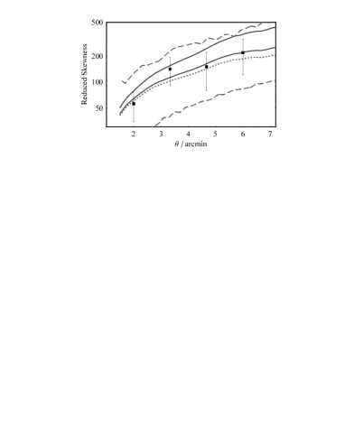
Figure 3: The measured reduced shear skewness (square with error bars) compared to cosmological models with standard gravity (dotted line for $\Lambda$-CDM, upper dashed line for open CDM and lower dashed line for standard CDM) or with modified gravity for $\Lambda$ CDM, $r_{s}=10h^{-1}$ Mpc (lower solid line) and $r_{s}=2h^{-1}$ Mpc (upper solid line).

It happens that quantities directly related to the reduced third moment of the potential Laplacian have been measured in cosmic shear catalogues [29]. The three-point correlation of the shear field (or rather some geometrical average of it) has been detected with a significant confidence level (through a rather elaborate procedure) at different angular scales [30]. If one applies the scaling law one expects for modified gravity to the predictions of standard gravity (in a $\Lambda$ dominated universe) it is possible to put constraints on $r_{s}$. From Fig. 3 it appears that current data already disfavor values of $r_{s}$ below $2h^{-1}$ Mpc although it is probably impossible to put a definitive statement from this data set. The constraints on the scale at which modified gravity intervenes are however strongly dependent on the modelling of the observations, and on the detailed shape of the 4D to 5D transition.

Cosmic shear surveys appear nonetheless very attractive to test the validity of the Einstein gravity law at cosmological scales. The fact such surveys provide us with genuine potential distribution at large scale makes them precious probes of the gravitational instability mechanisms in general. Undoubtedly, much stringent constraints should be obtainable from the coming cosmic shear surveys such as the CFHTLS or on the long term satellite missions like JDEM/SNAP.

Note that should such a modified gravity be the reason of the observed evidences of an accelerated universe $r_{s}$ would be expected to be the order of the Hubble size. Obtaining constraints on $r_{s}$ of this order form large-scale surveys may not be as hopeless at it seems. For the potential shape derived in [14] parameterized by a scale $r_{c}$ whose estimated value is $r_{c}=1.2\,c/H_{0}$ [15], the amplification of the three-point correlation is not as small for the available scales as the simplified model used here suggests. At 10 $h^{-1}$Mpc scale the effect would be at percent level; at 100 $h^{-1}$Mpc scale, it would reach 7% (a valid theory of gravity has however to be done in those models). If this approach reveals the only way to distinguish between quintessence type and modified gravity models to account for the dark energy evidences, it calls for the realization of very large - possibly whole sky - cosmic shear surveys.

References

- [1] Spergel et al. for the WMAP collaboration, Astrophys. J. Suppl. 148 (2003) 175
- [2] A. Lue, R. Scoccimarro, G. Starkman, Phys. Rev. D69 (2004) 044005
- [3] L. Randall and R. Sundrum, Phys. Rev. Lett. 83 (1999) 3370; ibid. 83 (1999) 4690.
- [4] P. Binétruy, C. Deffayet, and D. Langlois, Nucl. Phys. B565 (2000) 269.
- [5] R. Gregory, V.A. Rubakov, and S.M. Sibiryakov, Phys. Rev. Lett. 84 (2000) 5928
- [6] I.I. Kogan, S. Mouslopoulos, A. Papazoglou, G. G. Ross, J. Santiago, Nucl. Phys. B584 (2000) 313.
- [7] E. Fischbach and C. Tamadge The search for non Newtonian Gravity (AIP Springer-Verlag, New York, 1999); Y.T. Chen and A. Cook, Gravitational experiments in the laboratory (Cambridge University Press, New York, 1993).
- [8] I. Ciufolini and J.A. Wheeler, Gravitation and inertia (Princeton University Press, Princeton, 1995); C.M. Will, Theory and experiment in gravitational physics, (Cambridge University Press, New York, 1993).
- [9] J.C. Long, H.W. Chan, and J.C. Price, Nucl. Phys. B539 (1999) 23; S.R. Beane, Gen. Rel. Grav. 29 (1997) 945; S. Dimopoulos and G.F. Giudice, Phys. Lett. B379 (1996) 105.
- [10] For a recent review of experimental tests of GR see T. Damour, Nucl. Phys. Proc. Suppl. 80 (2000) 41.
- [11] S.W. Allen, S. Ettori, and A.C. Fabian [astro-ph/0008517].
- [12] N. Arkani-Hamed, S. Dimopoulos, and G. Dvali, Phys. Lett. B429 (1998) 263; Phys. Rev. D59 (1999) 086004; I. Antoniadis et al., Phys. Lett. B436 (1998) 257.
- [13] J. Garriga and T. Tanaka, Phys. Rev. Lett. 84 (2000) 2778; D.J.H. Chung, L. Everett and H. Davoudiasl, Phys. Rev. D64 (2001) 065002.
- [14] C. Deffayet, Phys. Lett. B 502 (2001) 199; C. Deffayet, G. Dvali, G. Gabadadze, Phys. Rev. D65 (2002) 044023
- [15] C. Deffayet, S.J. Landau, J. Raux, M. Zaldarriaga, P. Astier, Phys. Rev. D66 (2002) 024019
- [16] J.-P. Uzan, N. Aghanim, Y. Mellier, [astro-ph/0405620]
- [17] J.-P. Uzan, F. Bernardeau, Phys. Rev. D64 (2001) 083004
- [18] F. Perrotta, S. Matarrese, M. Pietroni, C. Schimd, Phys.Rev. D69 (2004) 084004; L. Amendola Phys. Rev. D69 (2004) 103524; V. Acquaviva, C. Baccigalupi, F. Perrotta, Phys. Rev. D70 (2004) 023515.
- [19] S.L. Dubovsky, V.A. Rubakov, and P.G. Tinyakov, Phys. Rev. D62 (2000) 105011.
- [20] P. Binétruy and J. Silk, Phys. Rev. Lett. 87 (2001) 031102.
- [21] P.J.E. Peebles, The Large Scale Structure of the Universe (Princeton University Press, Princeton, NJ, 1980); F. Bernardeau, S. Colombi, E. Gaztañaga, R. Scoccimarro, Phys.Rept. 367 (2002) 1
- [22] Y. Mellier, Annu. Rev. Astron. Astrophys. 37 (1999) 127.
- [23] M. Bartelmann and P. Schneider, Physics Reports 340 (2001) 291, and ref. therein.
- [24] L. Van Waerbeke et al., Astron. Astrophys. 358 (2000) 30; N. Kaiser, G. Wilson, and G.A. Luppino, [astro-ph/0003338]; D. Bacon, A. Refregier, and A. Ellis, Month. Not. R. Astron. Soc. 318 (2000) 625; D. Wittman et al., Nature 405 (2000) 143.
- [25] V. Narayanan, A. Berlind and D. Weinberg, Astrophys. J. 528 (2000) 1.
- [26] C. Sealfon, L. Verde, R. Jimenez [astro-ph/0404111]
- [27] A. Lue, R. Scoccimarro, G.D. Starkman, Phys.Rev. D69 (2004) 124015.
- [28] H.A. Feldman, J.A. Frieman, J.N. Fry, R. Scoccimarro, Phys. Rev. Lett. 86 (2001) 1434
- [29] F. Bernardeau, Y. Mellier, L. van Waerbeke, Astron. Astrophys. Lett., 389 (2002) L28; U.-L. Pen, T. Zhang, L. van Waerbeke, Y. Mellier, P. Zhang, J. Dubinski, Astrophys. J., 592 (2003) 664
- [30] F. Bernardeau, Y. Mellier, L. van Waerbeke, Astron. Astrophys., 397 (2003) 405