Solar System Science with SKA

Abstract

Radio wavelength observations of solar system bodies reveal unique information about them, as they probe to regions inaccessible by nearly all other remote sensing techniques and wavelengths. As such, the SKA will be an important telescope for planetary science studies. With its sensitivity, spatial resolution, and spectral flexibility and resolution, it will be used extensively in planetary studies. It will make significant advances possible in studies of the deep atmospheres, magnetospheres and rings of the giant planets, atmospheres, surfaces, and subsurfaces of the terrestrial planets, and properties of small bodies, including comets, asteroids, and KBOs. Further, it will allow unique studies of the Sun. Finally, it will allow for both indirect and direct observations of extrasolar giant planets.

1 Introduction

Radio wavelength observations of solar system bodies are an important tool for planetary scientists. Such observations can be used to probe regions of these bodies which are inaccessible to all other remote sensing techniques. For solid surfaces, depths of up to meters into the subsurface are probed (the rough rule of thumb is that depths to $\sim$10 wavelengths are sampled). For giant planet atmospheres, depths of up to 10’s of bars are probed. Probing these depths yields unique insights into the bodies, their composition, physical state, dynamics, and history. The ability to resolve this emission is important in such studies. The VLA has been the state-of-the-art instrument in this respect for the past 20 years, and its power is evidenced by the body of literature in planetary science utilizing its data. With its upgrade (to the EVLA), it will remain in this position in the near future. However, even with that upgrade, there are still things beyond its capabilities. For these studies, the SKA is the only answer. We investigate the capabilities of SKA for solar system studies below, including studies of the Sun. We also include observations of extrasolar giant planets. Such investigations have appeared before (for example, in the EVLA science cases in a general sense, and more specifically in de Pater (1999)), and we build on those previous expositions here.

2 Instrumental Capabilities

For solar system work the most interesting frequencies in most cases are the higher ones, since the sources are mostly blackbodies to first order (see discussion below for exceptions). We are very interested in the emission at longer wavelengths, of course, but the resolution and source detectability are maximized at the higher frequencies. To frame the discussion below, we need to know what those resolutions and sensitivities are. We take our information from the most recently released SKA specifications (Jones 2004).

The current specifications for SKA give a maximum baseline of 3000 km. Given that maximum baseline length, Table 1 shows the resolution of SKA at three values of the maximum baseline, assuming we can taper to the appropriate length if desired. In subsequent discussion we will translate these resolutions to physical dimensions at the distances of solar system bodies.

Table 1: Resolution in masec for SKA.

$\nu$ (GHz)	$\theta_{300}$	$\theta_{1000}$	$\theta_{3000}$
0.5	410	120	40
1.5	140	40	14
5	40	12	4
25	8	3	1

The specification calls for $A/T$ of 5000 at 200 MHz; 20000 from 500 MHz to 5 GHz; 15000 at 15 GHz; and 10000 at 25 GHz. The specification also calls for 75% of the collecting area to be within 300 km. Let us assume that 90% of the collecting area is within 1000 km. The bandwidth specification is 25% of the center frequency, up to a maximum of 4 GHz, with two independently tunable passbands and in each polarization (i.e., 16 GHz total bandwidth at the highest frequencies). Given these numbers, we can then calculate the expected flux density and brightness temperature noise values, as shown in Table 2.

Table 2: Sensitivities for SKA in nJy and K in 1 hour of observing.

$\nu$ (GHz)	${\Delta}F_{300}$	${\Delta}T_{B_{300}}$	${\Delta}F_{1000}$	${\Delta}T_{B_{1000}}$	${\Delta}F_{3000}$	${\Delta}T_{B_{3000}}$
0.5	97	2.3	81	22	73	170
1.5	56	1.3	47	12	42	100
5	31	0.7	26	6.8	23	55
25	34	0.8	29	7.6	26	62

3 Giant Planets

Observations of the giant planets in the frequency range of SKA are sensitive to both thermal and nonthermal emissions. These emissions are received simultaneously, and can be distinguished from each other by examination of their different spatial, polarization, time (e.g., for lightning), and spectral characteristics. Given the sensitivity and resolution of SKA (see Table 3), detailed images of both of these types of emission will be possible. We note, however, the difficulty in making images with a spatial dynamic range of $>$ 1000 (take the case of Jupiter, with a diameter of 140000 km, and resolution of $\sim$100 km) - this will be challenging, not only in the measurements (good short spacing coverage - down to spacings of order meters - is required), but in the imaging itself.

Table 3: SKA linear resolution for giant planets.

	Distance	resolution (km) ∗
Body	(AU)	$\nu=$2 GHz	$\nu=$20 GHz
Jupiter	5	120	10
Saturn	9	210	20
Uranus	19	420	40
Neptune	30	690	70

^∗ assuming maximum baseline of 1000 km

3.1 Nonthermal emission

Nonthermal emissions from the giant planets at frequencies between 0.15 and 20 GHz are limited to synchrotron radiation and atmospheric lightning. Both topics have been discussed before in connection to SKA by de Pater (1999). We review and update these discussions here.

3.1.1 Synchrotron radiation

Synchrotron radiation results from energetic electrons ($\sim$ 1-100 MeV) trapped in the magnetic fields of the giant planets. At present, synchrotron emission has only been detected from Jupiter, where radiation at wavelengths longer than about 6 cm is dominated by this form of emission (Berge & Gulkis 1976). Saturn has no detectable synchrotron radiation because the extensive ring system, which is almost aligned with the magnetic equatorial plane, absorbs energetic particles (McDonald, Schardt, & Trainor 1980). Both Uranus and Neptune have relatively weak magnetic fields, with surface magnetic field strengths $\sim$20-30 times weaker than Jupiter. Because the magnetic axes make large angles (50-60^∘) with the rotational axes of the planets, the orientation of the field of Uranus with repect to the solar wind is in fact not too dissimilar from that of Earth (because its rotational pole is nearly in the ecliptic), while the magnetic axis of Neptune is pointed towards the Sun once each rotation period. These profound changes in magnetic field topology have large effects on the motion of the local plasma in the magnetosphere of Neptune. It is unclear if there is a trapped population of high energy electrons in the radiation belt of either planet, a necessary condition for the presence of synchrotron radiation. Before the Voyager encounter with the planet, de Pater & Goertz (1989) postulated the presence of synchrotron radiation from Neptune. Based on the calculations in their paper, the measured magnetic field strengths, and 20-cm VLA observations (see, e.g., de Pater, Romani, & Atreya 1991) we would estimate any synchrotron radiation from the two planets not to exceed $\sim$0.1 mJy. This, or even a contribution one or two orders of magnitude smaller, is trivial to detect with the SKA. It would be worthwhile for the SKA to search for potential synchrotron emissions off the disks of Uranus and Neptune (and SKA can easily distinguish the synchrotron emission from that from the disk based on the spatial separation), since this information would provide a wealth of information on the inner radiation belts of these planets.

Jupiter’s synchrotron radiation has been imaged at frequencies between 74 MHz and 22 GHz (see, e.g., de Pater 1991; de Pater, Schulz, & Brecht 1997; Bolton et al. 2002; de Pater & Butler 2003; de Pater & Dunn 2003). A VLA image of the planet’s radio emission at $\lambda=20$ cm is shown in Figure 1a; the spatial distribution of the synchrotron radiation is very similar at all frequencies (de Pater & Dunn 2003). Because the radio emission is optically thin, and Jupiter rotates in 10 hours, one can use tomographic techniques to recover the 3D radio emissivity, assuming the emissions are stable over 10 hours. An example is shown in Figure 1b (Sault et al. 1997; Leblanc et al. 1997; de Pater & Sault 1998). The combination of 2D and 3D images is ideal to deduce the particle distribution and magnetic field topology from the data (Dulk et al. 1997; de Pater & Sault 1998; Dunn, de Pater, & Sault 2003).

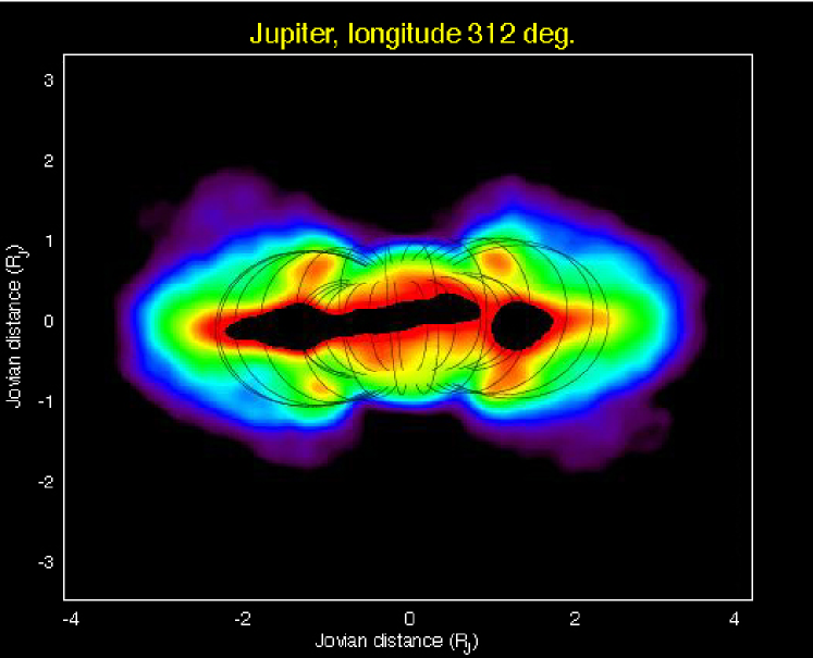
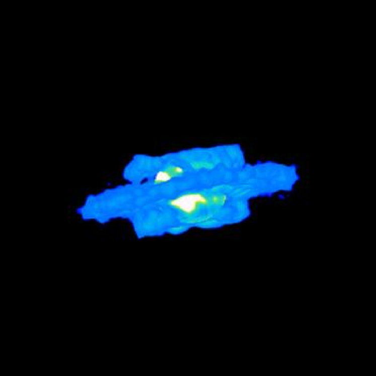
Figure 1: Radio images of Jupiter’s synchrotron emission. a) (left) Image made from VLA data taken at a frequency of 1450 MHz. Both the thermal (confined to Jupiter’s disk) and nonthermal emisions are visible. The resolution is $\sim$0.3 $R_{J}$, roughly the size of the high latitude emission regions. Magnetic field lines from a magnetic field model are superposed, shown every $15^{\circ}$ of longitude. After de Pater, Schulz, & Brecht (1997). b) (right) Three-dimensional reconstruction of the June 1994 data, as seen from Earth. The planet is added as a white sphere in this visualization. After de Pater & Sault (1998).

The shape of Jupiter’s radio spectrum is determined by the intrinsic spectrum of the synchrotron radiating electrons, the spatial distribution of the electrons and Jupiter’s magnetic field. Spectra from two different years (1994 and 1998) are shown in Figure 2 (de Pater et al. 2003; de Pater & Dunn 2003). The spectrum is relatively flat shortwards of 1-2 GHz, and drops off more steeply at higher frequencies. As shown, there are large variations over time in the spectrum shortwards of 1-2 GHz, and perhaps also at the high frequencies, where the only two existing datapoints at 15 GHz differ by a factor of $\sim$3. Changes in the radio spectrum most likely reflect a change in either the spatial or intrinsic energy distribution of the electrons. The large change in spectral shape between 1994 and 1998 has been attributed to pitch angle scattering by plasma waves, Coulomb scattering and perhaps energy degradation by dust in Jupiter’s inner radiation belts, processes which affect in particular the low energy distribution of the electrons. With SKA we may begin investigating the cause of such variability through its imaging capabilities at high angular resolution, and simultaneous good u-v coverage at short spacings. As shown by de Pater (1999), this is crucial for intercomparison at different frequencies. With such images we can determine the spatial distribution of the energy spectrum of electrons, which is tightly coupled to the (still unknown) origin and mode of transport (including source/loss terms) of the high energy electrons in Jupiter’s inner radiation belts.

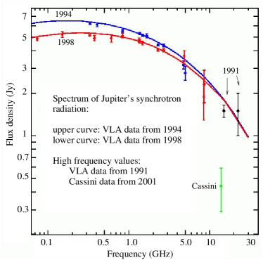
Figure 2: The radio spectrum of Jupiter’s synchtrotron emission as measured in September 1998 (lower curve) and June 1994 (upper curve), with high frequency data points from March 1991 (VLA) and January 2001 (Cassini; Bolton et al. 2002). Superposed are model calculations that match the data (Adapted from de Pater & Dunn 2003).

3.1.2 Lightning

Lightning appears to be a common phenomenon in planetary atmospheres. It has been observed on Earth, Jupiter, and possibly Venus (Desch et al. 2002). Electrostatic discharges on Saturn and Uranus have been detected by spacecraft at radio wavelengths, and are probably caused by lightning. The basic mechanism for lightning generation in planetary atmospheres is believed to be collisional charging of cloud droplets followed by gravitational separation of oppositely charged small and large particles, so that a vertical potential gradient develops. The amount of charges that can be separated this way is limited; once the resulting electric field becomes strong to ionize the intervening medium, a rapid ’lightning stroke’ or discharge occurs, releasing the energy stored in the electric field. For this process to work, the electric field must be large enough, roughly of the order of 30 V per electron mean free path in the gas, so that an electron gains sufficient energy while traversing the medium to cause a collisional ionization. When that condition is met, a free electron will cause an ionization at each collision with a gas molecule, producing an exponential cascade (Gibbard et al. 1999).

In Earth’s atmosphere, lightning is almost always associated with precipitation, although significant large scale electrical discharges also occur occasionally in connection with volcanic eruptions and nuclear explosions. By analogy, lightning on other planets is only expected in atmospheres where both convection and condensation take place. Moreover, the condensed species, such as water droplets, must be able to undergo collisional charge exchange. It is possible that lightning on other planets is triggered by active volcanism (such as possibly on Venus or Io).

We believe that SKA would be an ideal instrument to search for lightning on other planets; the use of multiple beams would facilitate discrimination against lightning in our own atmosphere, and simultaneous observations at different frequencies would contribute spectral information. For such experiments one needs high time resolution (as for pulsars) and the ability to observe over a wide frequency range simultaneously, including in particular the very low frequencies ($<$ 300 MHz).

3.2 Thermal emission

The atmospheres of the giant planets all emit thermal (blackbody) radiation. At radio wavelengths most of the atmospheric opacity has been attributed to ammonia gas, which has a broad absorption band near 22 GHz. Other sources of opacity are collision induced absorption by hydrogen, H₂S, PH₃, H₂O gases, and possibly clouds. Since the overall opacity is dominated by ammonia gas, it decreases approximately with $\nu^{-2}$ for $\nu<22$ GHz. One therefore probes deeper warmer layers in a planet’s atmosphere at lower frequencies. Spectra of all four giant planets have been used to extract abundances of absorbing gases, in particular NH₃, and for Uranus and Neptune, H₂S (H₂S has been indirectly inferred for Jupiter and Saturn) (see, e.g., Briggs & Sackett 1989; de Pater, Romani, & Atreya 1991; de Pater & Mitchell 1993; DeBoer & Steffes 1996).

The thermal emission from all four giant planets has been imaged with the VLA. To construct high signal-to-noise images, the observations need to be integrated over several hours, so that the maps are smeared in longitude and only reveal brightness variations in latitude. The observed variations have typically been attributed to spatial variations in ammonia gas, as caused by a combination of atmospheric dynamics and condensation at higher altitudes. Recently, Sault, Engel, & de Pater (2004) developed an algorithm to construct longitude-resolved images; they applied this to Jupiter, and their maps reveal, for the first time, hot spots at radio wavelengths which are strikingly similar to those seen in the infrared (Figure 3). At radio wavelengths the hot spots indicate a relative absence of NH₃ gas, whereas in the infrared they suggest a lack of cloud particles. The authors showed that the NH₃ abundance in hot spots was depleted by a factor of 2 relative to the average NH₃ abundance in the belt region, or a factor of 4 compared to zones. Ammonia must be depleted down to pressure levels of $\sim$5 bar in the hot spots, the approximate altitude of the water cloud. The algorithm of Sault, Engel, & de Pater (2004) only works on short wavelength data of Jupiter, where the synchrotron radiation is minimal.

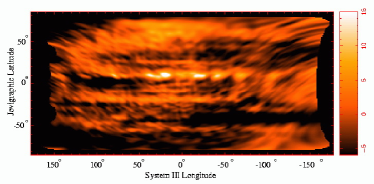
Figure 3: Longitude-resolved image of Jupiter at 2 cm (Sault, Engel, & de Pater 2004).

Even the longitudinally smeared images are important in deducing the state of the deep atmospheres of the giant planets, as attested by numerous publications on the giant planets. Here we discuss specifically the case of Uranus, where radio images made with the VLA since 1981 at 2 and 6 cm have shown changes in the deep atmosphere which appear to be related to the changing insolation as the two poles rotate in and out of sunlight over the 40 year uranian year. Since the first images were made, the south pole has appeared brighter than equatorial regions. In the last decade, however, the contrast between the two regions and the latitude at which the transition occurs has changed (Hofstadter & Butler 2003). Figure 4 shows an image from the VLA made from data taken in the summer of 2003, along with an image at near-infrared wavelengths (1.6 $\mu$m) taken with the adaptive optics system on the Keck telescope in October 2003 (Hammel et al. 2004). The VLA image clearly shows that the south pole is brightest, but it also shows enhanced brightness in the far-north (to the right on the image). At near-infrared wavelengths Uranus is visible in reflected sunlight, and hence the bright regions are indicative of clouds/hazes at high (upper troposphere) altitudes, presumably indicative of rising gas (with methane condensing out). We note that the bright band around the south pole is at the lower edge of the VLA-bright south polar region. It appears as if air is rising (with condensibles forming clouds) along the northern edge of the south polar region and descending over the pole, where the low radio opacity is indicative of dry air.

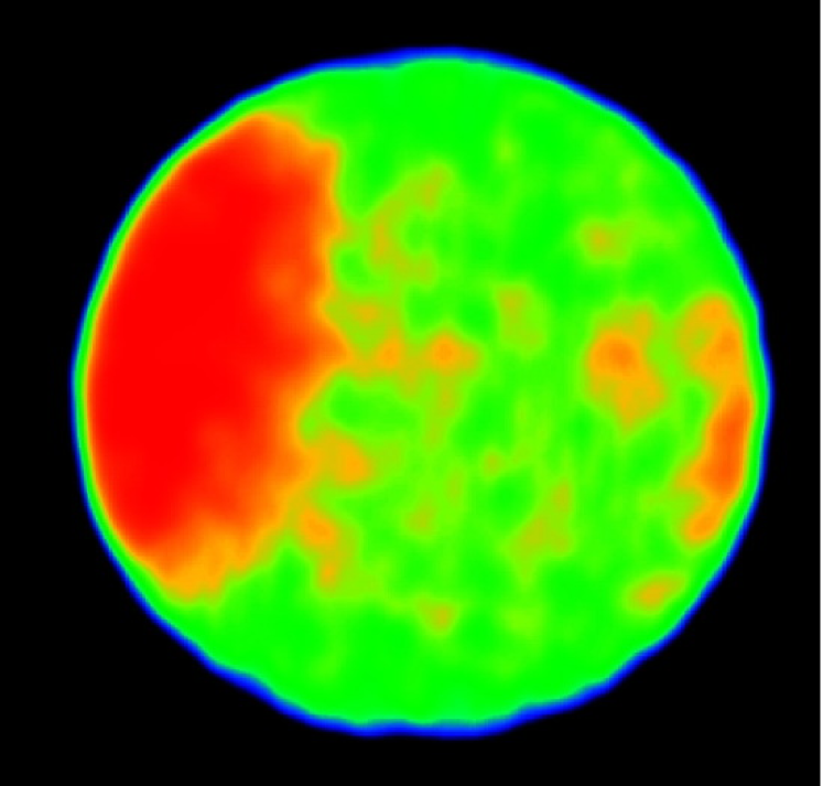
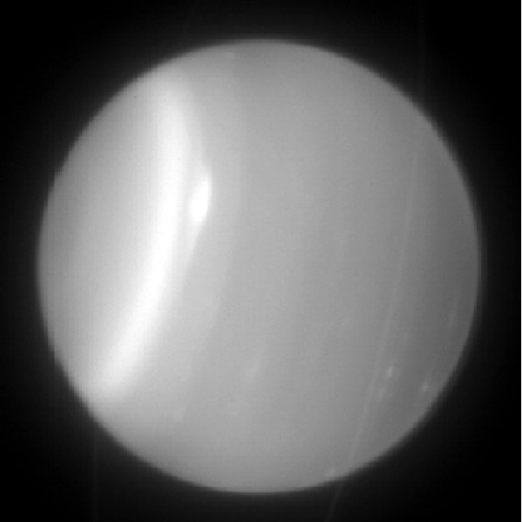
Figure 4: Two panels comparing VLA (left, Hofstadter & Butler 2004) and Keck (right, Hammel et al. 2004) images of Uranus from the summer of 2003. In the radio image, red is brighter, cycling to lower brightness through orange, yellow, green, blue, and black. Note the edge of the radio bright region in the south (to the left in the images) corresponds to a prominent band in the infrared. The radio bright region in the north has no corresponding band. The faint line across the planet on the right-hand side of the infrared image is the ring system.

With a sensitivity of SKA 2 orders of magnitude better than that of the VLA, and excellent instantaneous UV coverage, images of a planet’s thermal emission can be obtained within minutes, rather than hours. This would enable direct mapping of hot spots at a variety of frequencies, including low frequencies where both thermal and nonthermal radiation is received. We can thus obtain spectra of hot spots, which allow us to derive the altitude distribution of absorbing gases, something that hitherto could only be obtained via in situ probes. Equally exciting is the prospect of constructing complete 3D maps of the ammonia abundance (or total opacity, to be precise) at pressure levels between 0.5 and $\sim$ 20-50 bars (these levels vary some from planet to planet). Will ammonia, and other sources of opacity, be homogeneous in a planet’s deep atmosphere (i.e., at pressure levels $\;\buildrel>\over{\scriptstyle\sim}\;$ 10 bar)? Could there be giant thunderstorms rising up from deep down, bringing up concentrations of ammonia and other gases from a planet’s deep atmosphere, i.e., reflecting the true abundance at deep levels? Such scenarios have been theorized for Jupiter, but never proven (Showman & de Pater 2004).

A cautionary note here: although excellent images at multiple wavelengths yield, in principle, information on a giant planet’s deep atmosphere, detailed modeling will be frustrated in part because of a lack of accurate laboratory data on gases and clouds that absorb at microwave frequencies, such as NH₃ and H₂O. This severely limits the precision at which one can separate contributions from different gases. Planetary scientists are in particular eager to deduce the water abundance in a planet’s deep atmosphere (e.g., Jupiter). The potential of deriving the water abundance in the deep atmosphere of Jupiter from microwave observations was reviewed by de Pater et al. (2004), while Janssen et al. (2004) investigated the potential of using limb darkening measurements on a spinning spacecraft. These studies show that it might be feasible to extract limits on the water abundance in the deep atmosphere, but only if the absorption profile of water and ammonia gas is accurately known.

3.3 Rings

Planetary rings emit thermal radiation, but this contribution is very small compared to the planet’s thermal emission reflected from the rings. Although all 4 giant planets have rings, radio emissions have only been detected from Saturn’s rings. Other rings are too tenuous to reflect detectable amounts of radio emissions (Jupiter’s synchrotron radiation, though, does reflect the presence of its ring via absorption of energetic electrons). Several groups have gathered and analyzed VLA data of Saturn’s rings over the past decades (see, e.g., Grossman, Muhleman, & Berge 1989; van der Tak et al. 1999; Dunn, Molnar, & Fix 2002). These maps, at frequencies $>$ a few GHz, are usually integrated over several hours, and reveal the classical A, B, and C rings including the Cassini Division. Asymmetries, such as wakes, have been detected in several maps; research is ongoing as to correlations between observed asymmetries with wavelength and ring inclination angle.

With the high sentivity, angular resolution and simultaneous coverage of short u-v spacings, maps of Saturn’s rings can be improved considerably. This would allow higher angular resolution and less longitudinal smearing, allowing searches for longitudinal inhomogeneities. In addition, it may become feasible to detect the uranian $\epsilon$ ring and perhaps even the main ring of Jupiter during ring plane crossings. We note that the detection of the Jupiter ring is made difficult by being so faint and close to an extremely bright Jupiter.

4 Terrestrial Planets

Radio wavelength observations of the terrestrial planets (Mercury, Venus, the Moon, Mars) are important tools for determining atmospheric, surface and subsurface properties. For surface and subsurface studies, such observations can help determine temperature, layering, thermal and electrical properties, and texture. For atmospheric studies, such observations can help determine temperature, composition, and dynamics. Given the sensitivity and resolution of SKA (see Table 4), detailed images of both of these types of emission will be possible. We note, however, similarly to the giant planet case above, the difficulty in making images with a spatial dynamic range of $>$ 10000 (take the case of Venus, with a diameter of 12000 km, and resolution of $\sim$1 km). The Moon is a special case, where mosaicing will likely be required, the emission is bright and complicated, and it is in the near field of SKA (in fact, many of the planets are in the near field formally, but the Moon is an extreme case). The VLA has been used to image the Moon (Margot et al. 1997), and near field imaging techniques are being advanced (Cornwell 2004), but imaging of the Moon will be a challenge for SKA.

Table 4: SKA linear resolution for terrestrial planets.

	Distance	resolution (km) ∗
Body	(AU)	$\nu=$2 GHz	$\nu=$20 GHz
Moon	0.002	0.015	0.004
Venus	0.3	2	0.7
Mercury, Mars	0.6	4	1.3

^∗ assuming maximum baseline of 1000 km

4.1 Surface and subsurface

The depth to which temperature variations penetrate in the subsurface is characterized by its thermal skin depth, where the magnitude of the diurnal temperature variation is decreased by 1/e:  $l_{t}=\sqrt{kP/(\pi C_{p}\rho)}$, where $k$ is the thermal conductivity, $P$ is the rotational period, $\rho$ is the mass density, and $C_{p}$ is the heat capacity. For the terrestrial planets, using thermal properties of lunar soils and the proper rotation rates, the skin depths are of order a few cm (Earth and Mars) to a few 10’s of cm (Moon, Mercury, and Venus, because of their slow rotation). The 1/e depth to which a radio wavelength observation at wavelength $\lambda$ probes in the subsurface is given by:  $l_{r}=\lambda/(2\pi\sqrt{\epsilon_{r}}\tan\Delta)$, where $\epsilon_{r}$ is the real part of the dielectric constant, and $\tan\Delta$ is the “loss tangent” of the material - the ratio of the imaginary to the real part of the dielectric. For all of the terrestrial planets, given reasonable regolith dielectric constant, this is roughly 10 wavelengths. So, the wavelengths of SKA are well matched to probing both above and below the thermal skin depths of the terrestrial planets.

The thermal emission from Mercury has been mapped with the VLA and BIMA by Mitchel & de Pater (1994), who determined that not only was the subsurface probably layered, but that the regolith is likely relatively basalt free. Figure 5 shows a VLA observation, compared with the detailed model of Mitchell & de Pater. Observations with SKA will further determine our knowledge of these subsurface properties. Furthermore, given the 1 km resolution, mapping of the near-surface temperatures of the polar cold spots (inferred from the presence of odd radar scattering behavior - Harmon, Perillat, & Slade 2001) will be possible, a valuable constraint on their composition. Finally, given accurate enough (well calibrated, on an absolute scale) measurements, constraints on the presence or absence of an internal dynamo may be placed.

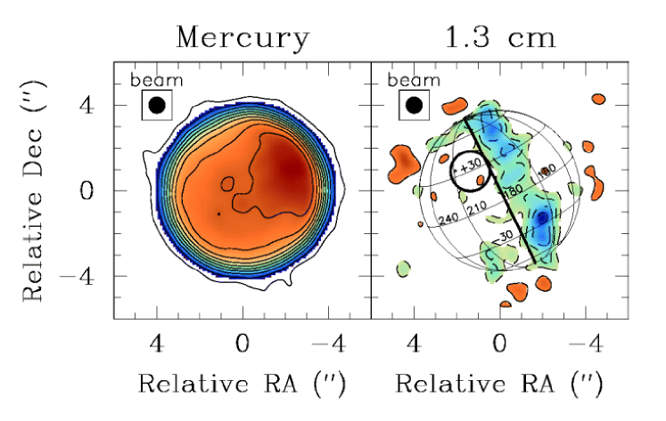
Figure 5: Image of Mercury at 1.3 cm made from data taken at the VLA (Mitchel & de Pater 1994). The left panel shows the image, where red is brighter (hotter), cycling to lower brightness through orange, yellow, green, blue, and purple to white. The right panel shows this image after subtraction of a detailed model. The solid line is the terminator, the circle is Caloris basin. The model does well except at the terminator and in polar regions, most likely because of unmodelled topography and surface roughness.

The question of the long wavelength emission from Venus could be addressed by SKA observations. Recent observations have verified that the emission from Venus at long wavelengths ($\;\buildrel>\over{\scriptstyle\sim}\;$ 6 cm) are well below predicted - by up to 200 K (Butler & Sault 2003). Figure 6 shows this graphically. There is currently no explanation for this depression. Resolved images at long wavelengths (say 500 MHz, where the resolution of SKA is of order 100 km at the distance of Venus using only the 300 km baselines and less, and the brightness temperature sensitivity is about 3 K in 1 hour) will help in determining whether this is a global depression, or limited to particular regions on the planet.

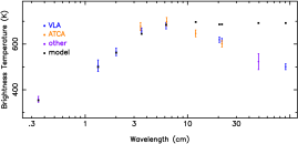
Figure 6: Microwave brightness temperature spectrum of Venus, from Butler & Sault (2003). The depression of the measured emission compared to models at long wavelengths, up to 200 K, is evident.

Although NASA has been sending multiple spacecraft to Mars, there are still uses for Earth-based radio wavelength observations. To our knowledge, there is currently no planned microwave mapper for a Mars mission, other than the deep sounding very long wavelength radar mappers (MARSIS, for example). So observations in the meter-to-cm wavelength range are still important for deducing the properties of the important near-surface layers of the planet. Observations of the seasonal caps as they form and subsequently recede would provide valuable constraints on their structure. Observations of the odd “stealth” region (Edgett et al. 1997) would help constrain its composition and structure, and in combination with imagery constrain its emplacement history.

4.2 Atmosphere

The Moon and Mercury have no atmosphere to speak of, but Venus and Mars will both benefit from SKA observations of their atmospheres. Short wavelength observations of the venusian atmosphere ($\;\buildrel<\over{\scriptstyle\sim}\;$ 3 cm) probe the lower atmosphere, below the cloud layer ($\;\buildrel<\over{\scriptstyle\sim}\;$ 40 km). Given the abundance of sulfur-bearing molecules in the atmosphere, and their high microwave opacity, such observations can be used to determine the abundances and spatial distribution of these molecules. Jenkins et al. (2002) have mapped Venus with the VLA at 1.3 and 2 cm, determining that the below-cloud abundance of SO₂ is lower than that inferred from infrared observations, and that polar regions have a higher abundance of H₂SO₄ vapor than equatorial regions, supporting the hypothesis of Hadley cell circulation. VLA observations are hampered both by sensitivity and spatial dynamic range. The EVLA will solve part of the sensitivity problem, but will not solve the instantaneous spatial dynamic range problem - only the SKA can do both. Given SKA observations, cloud features (including at very small scales), and temporal variation of composition (which could be used as as proxy to infer active volcanism, since it is thought that significant amounts of sulfur-bearing molecules would be released in such events) could be sensed and monitored.

Observations of the water in the Mars atmosphere with the VLA have provided important constraints on atmospheric conditions and the climate of the planet (Clancy et al. 1992). The 22 GHz H₂O line is measured, and emission is seen along the limb, where pathlengths are long (this fact is key - the resolution of the atmosphere along the limb is critical). Figure 7 shows an image of this. For added sensitivity in these kinds of observations (needed to improve the deduction of temperature and water abundance in the atmosphere), only the SKA will help.

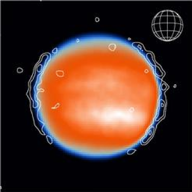
Figure 7: Map of water vapor in the Mars atmosphere made from data taken at the VLA in 1991. The colored background is the thermal emission from the surface. The contours are the H₂O emission, seen only along the limb. From Clancy et al. (1992).

5 Large Icy Bodies

In addition to their odd radar scattering properties (see the Radar section below), the Galilean satellites Europa and Ganymede exhibit unusually low microwave emission (de Pater, Brown, & Dickel 1984; Muhleman et al. 1986; Muhleman & Berge 1991). Observations with SKA will determine the deeper subsurface properties of the Galilean satellites, Titan, the larger uranian satellites, and even Triton, Pluto, and Charon. For example, given a resolution of 40 km at 20 GHz (appropriate for the mean distance to Uranus), maps of hundreds of pixels could be made of the uranian moons Titania, Oberon, Umbriel, Ariel, and Miranda. Pushing to 3000 km baselines, maps of tens of pixels could even be made of the newly discovered large KBOs Quaoar and Sedna (Quaoar is estimated to be $\sim$40 masec in diameter, Sedna about half that, (Brown & Trujillo 2004; Brown, Trujillo, & Rabinowitz 2004)). These bodies are some 10’s of K in physical temperature, probably with an emissivity of $\sim$0.9 (by analog with the icy satellites), so with a brightness temperature sensitivity of a few K in a few masec beam, SKA should have no problem making such maps with an SNR of the order of 10’s in each pixel. SKA will be unique in its ability to make such maps of these bodies - optical images will come nowhere near this resolution unless space-based interferometers become a reality.

6 Small Bodies

Perhaps the most interesting solar system science with SKA will involve the smaller bodies in the solar system. Because of their small size, their emission is weak, and they have therefore not been studied very extensively, particularly at longer wavelengths. Such bodies include the smaller satellites, asteroids, Kuiper Belt Objects (KBOs), and comets. These bodies are all important probes of solar system formation, and will yield clues as to the physical and chemical state of the protoplanetary and early planetary environment, both in the inner and outer parts of the solar system.

6.1 Small satellites

It is sometimes hypothesized that Phobos and/or Deimos are captured asteroids because of surface spectral reflectivity properties. This is inconsistent, however, with their current dynamical state and low internal density (see, e.g., the discussions in Burns 1992; Rivkin et al. 2002). The two moons could also have been formed via impact of a large asteroid into Mars, which could also have helped in forming the north-south dichotomy on the planet (Craddock 1994). Determination of the properties of the surface and near-surface could help unravel this mystery. These bodies are $\sim$10 km in diameter, so at opposition will be $\sim$30 masec in apparent diameter, so SKA will be able to map them with a few 10’s of pixels on the moons. This will provide some of these important properties and their variation as a function of location on the moons (notably regolith depth and thermal and electrical properties). As another example, consider the eight outer small jovian satellites, about which little is known, either physically or chemically. All eight of them, with diameters of from 15 to 180 km (Himalia), could be resolved by SKA at 20 GHz, determining their shapes as well as their surface and subsurface properties.

We note, however, that the imaging of these small satellites can be challenging, as they are often in close proximity to a very bright primary which may have complex brightness structure. As such, even with the specification that SKA must have a dynamic range of 10⁶, it will not be trivial to make images of these small, relatively weak satellites.

6.2 Main Belt Asteroids

The larger of the main belt asteroids are the only remaining rocky protoplanets (bodies of order a few hundred to 1000 km in diameter), the others having been dispersed or catastrophically disrupted, leaving the comminuted remnants comprising the asteroid belt today (Davis et al. 1979). They have experienced divergent evolutionary paths, probably as a consequence of forming on either side of an early solar system dew line beyond which water was a significant component of the forming bodies. Vesta is thought to have accreted dry, consequently experiencing melting, core formation, and volcanism covering its surface with basalt (Drake 2001). Ceres and Pallas, thermally buffered by water never exceeding 400K, experienced aqueous alteration processes evidenced by clay minerals on their surfaces (Rivkin 1997). These three large MBAs all reach apparent sizes of nearly 1^′′ at opposition, so maps with hundreds of pixels across them can be made, with high SNR (brightness temperature is of order 200 K, while brightness temperature sensitivity is of order a few K). Such maps will directly probe regolith depth and properties across the asteroids, yielding important constraints on formation hypotheses.

SKA will also be able to detect and map the smaller MBAs. Given the distances of the MBAs to the Sun, they typically have surface/sub-surface brightness temperatures (the brightness temperature is just the physical temperature multiplied by the emissivity) of $\sim$ 200 K. Given a typical distance (at opposition) of 1.5 AU, this gives diameters of 2, 20, and 200 masec for MBAs of 1, 10, and 100 km radius, with flux densities of 0.3, 30, and 3000 $\mu$Jy at $\lambda$ = 1 cm. So the larger MBAs will be trivial to detect and map, but the smallest of them will be somewhat more difficult to observe (but not beyond the sensitivity of SKA - see the discussion above on Instrumental Capabilities). There are more than 1500 MBAs with diameter $>$ 20 km just in the IRAS survey (Tedesco et al. 2002).

6.3 Near Earth Asteroids

In addition to being important remnants of solar system formation, NEAs are potential hazards to us here on Earth (Morbidelli et al. 2002). As such, their characterization is important (Cellino, Zappala, & Tedesco 2002). SKA will easily detect and image such asteroids. As they pass near the Earth, they are typically at a brightness temperature of 300 K, and pass at a distance of a few lunar radii ($\sim$0.005 AU). This distance gives diameters of 6, 60, and 600 masec for NEAs of 10, 100, and 1000 m, with flux densities of 0.005, 0.5, and 50 mJy $\mu$Jy at $\lambda$ = 1 cm. Again, these will be easily detected and mapped. ALMA will also be an important instrument for obseving these bodies (Butler & Gurwell 2001), but it is the combination of the data from ALMA and SKA that allows a complete picture of the surface and subsurface properties to be formed.

6.4 Kuiper Belt Objects

In general KBOs are detected at optical/near-IR wavelengths in reflected sunlight. Since the albedo of comet Halley was measured (by spacecraft) to be 0.04, comets/KBOs are usually assumed to have a similar albedo (which most likely is not true). This assumed albedo is then used to derive an estimate of the size based on the magnitude of the reflected sunlight. Resolved images, and hence size estimates, only exist of the largest KBOs (see, e.g., Brown & Trujillo 2004). The only other possibility (ignoring occultation experiments - Cooray 2003) to determine the size is via the use of radiometry, where observations of both the reflected sunlight and longer wavelength observations of thermal emission are used to derive both the albedo and radius of the object. This technique has been used, for example, for asteroids in the IRAS sample (Tedesco et al. 2002). Although more than 100 KBOs have been found to date, only two have been detected in direct thermal emission, at wavelengths around 1 mm (Jewitt, Aussel, & Evans 2001; Margot et al. 2002a) - the emission is simply too weak. ALMA will be an extremely important telescope for observing KBOs (Butler & Gurwell 2001), but will just barely be able to resolve the largest KBOs (with a resolution of 12 masec at 350 GHz in its most spread out configuration). SKA, with a resolution of a few masec and a brightness temperature sensitivity of a few K, will resolve all of the larger of the KBOs (larger than 100 km or so), and will easily detect KBOs with radii of 10’s of km. Combined observations with ALMA and SKA will give a complete picture of the surface, near-surface, and deeper subsurface of these bodies.

6.5 Comets

In addition to holding information on solar system formation, comets are also potentially the bodies which delivered the building blocks of life (both simple and complex organic molecules) to Earth. As such, they are important astronomical targets, as we would like to understand their current properties and how that constrains their history.

6.5.1 Nucleus

Long wavelengths (cm) are nearly unique in their ability to probe right to the surfaces of active comets. Once comets come in to the inner solar system, they generally produce so much dust and gas that the nucleus is obscured to optical, IR, and even mm wavelengths. At cm wavelengths, however, one can probe right to (and into) the nucleus of all but the most productive comets. For example, comet Hale-Bopp was detected with the VLA at X-band (Fernandez 2002). Given nucleus sizes of a few to a few 10’s of km, and distances of a few tenths to 1 AU, the flux densities from cometary nuclei should be from about 1 $\mu$Jy to 1 mJy at 25 GHz - easy to detect with SKA. Multi-wavelength observations should tell us not only what the surface and near-surface density is, but if (and how) it varies with depth. These nuclei should be roughly 10-100 masec in apparent size, so can be resolved at the high frequencies of SKA. With resolved images, in principle it would be possible to determine which areas were covered with active (volatile) material, i.e., ice, and which were covered with rocky material, and for the rocky material whether it was dust (regolith) or solid rock.

6.5.2 Ice and dust grain halo

Large particles (rocks and ice cubes) are clearly shed from cometary nuclei as they become active, as shown by radar observations (Harmon et al. 1999). The properties of these activity byproducts are important as they contain information on the physical structure and composition of the comets from which they are ejected. Observations at the highest SKA frequencies should be sensitive to emission from these large particles (even though they also probe down through them to the nucleus), and can thus be used to make images of these particles - telling us what the distribution (both spatially, and the size distribution of the particles) and total mass is, and how it varies with time.

6.5.3 Coma

Observations of cometary comae will tell us just what the composition of the comets is - both the gas to dust ratio, and the relative ratios of the volatile species. Historically, observations of cometary comae at cm wavelengths have been limited to OH, but with the sensitivity of SKA, other molecules such as formaldehyde (detected in comet Halley with the VLA - Snyder, Palmer, & de Pater 1989) and CH should be observable. The advantage of long wavelength transitions is that we observe rotational transitions of the molecules, which are much easier to understand and accurately characterize in the statistical equilibrium and radiative transfer models (necessary to turn the observed intensities into molecular abundances). Millimeter wavelength observations of cometary molecules have proven fertile ground (see, e.g., Biver et al. 2002), but the cm transitions of molecules are also important as they probe the most populous energy states, and some unique molecules which do not have observable transitions in the mm-submm wavelengths.

The volatile component of comets is $\sim$80% water ice, with the bulk of the rest CO₂. All other species are present only in small quantities. As the comet approaches the Sun, the water starts to sublimate, and along with the liberated dust forms the coma and tails. At 1 AU heliocentric distance, the typical escape velocity of the water molecules is 1 km/s, and the lifetime against dissociation is about 80000 sec, which leads to a water coma of radius 80000 km. Although there have been some claims of direct detection of the 22 GHz water line in comets, a very sensitive search for this emission from Hale-Bopp detected no such emission (Graham et al. 2000). With SKA, such observations should be possible and will likely be attempted. The problem is that the resolution is too high - with such a large coma, most of the emission will be resolved out.

Most of the water dissociates into H and OH. The hydroxyl has a lifetime of $1.6\times 10^{5}$ sec at 1 AU heliocentric distance, implying a large OH coma - of order 10^′ apparent size at 1 AU geocentric distance. The OH is pumped into disequilibrium by solar radiation, and acts as a maser. As such, the emission can be quite bright, and is regularly observed at cm wavelengths by single dishes as it amplifies the galactic or cosmic background (Schloerb & Gerard 1985). Since the spatial scale is so large, however, VLA observations of cometary OH have been limited to observations of only a few comets - Halley, Wilson, SL-2, and Hale-Bopp (de Pater, Palmer, & Snyder 1991; Butler & Palmer 1997). Figure 8 shows a VLA image of the OH emission from comet Halley. Though scant, these observations have helped demonstrate that the OH in cometary comae is irregularly distributed, likely due to quenching of the population inversion from collisions in the inner coma. Similar to the case for water above, SKA will resolve out most of this emission. It will certainly provide valuable observations of the distribution of OH in the inner coma, but not much better than is possible with the VLA currently. The real power of the SKA will be in observations of background sources amplified by the OH in the coma. The technique is described in Butler et al. (1997) and was demonstrated successfully for Hale-Bopp (Butler & Palmer 1997). Figure 9 shows example spectra. As a comet moves relative to a background source, the OH abundance along a chord through the coma is probed. Since the SKA will be sensitive to very weak background sources, many such sources should be available for tracking at any time, providing a nearly full 2-D map of the coma at high resolution (each chord is sampled along a pencil beam through the coma with diameter corresponding to the resolution of the interferometer at the distance of the comet). Combined with single-dish observations, this should provide a very accurate picture of the OH in cometary comae.

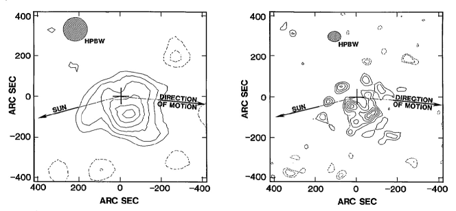
Figure 8: Images of the OH emission from comet Halley made with the VLA at low (left) and high (right) resolution. From de Pater, Palmer, & Snyder (1991).

Figure 9: Spectra of the OH emission from comet Hale-Bopp made as the comet occulted background sources. From Butler & Palmer (1997).

Among the five most common elements in cometary comae, the chemistry involving nitrogen is one of the least well understood (along with sulfur). In addition, ammonia is particularly important in terms of organic precursor molecules, and can also be used as a good thermometer for the location where comets formed - whether the nitrogen is in N₂ or NH₃ depends on the temperature of the local medium, among other things (Charnley & Rodgers 2002). Ammonia has a rich microwave spectrum which has been extensively observed in interstellar molecular clouds (see, e.g., Ho & Townes 1983). Observations of ammonia in cometary comae are therefore potentially very valuable in terms of determining current chemistry and formation history. Recently, comets Hyakutake and Hale-Bopp were observed in NH₃ (Bird et al. 1997; Hirota et al. 1999; Butler et al. 2002). Observations of cometary NH₃ will suffer from the same problem as the H₂O and OH - the NH₃ coma is large (although about a factor of 10 smaller than the water coma). However, if the individual elements are relatively small, and have any reasonable single dish capability, the NH₃ may still be detected.

7 Radar

Radar observations of solar system bodies contribute significantly to our understanding of the solar system. Radar has the potential to deliver information on the spin and orbit state, and the surface and subsurface electrical properties and texture of these bodies. The two most powerful current planetary radars are the 13 cm wavelength system on the 305 m Arecibo telescope and the 3.5 cm system on the 70 m Goldstone antenna. A radar that made use of the SKA for both transmitting and receiving the echo would have a sensitivity many hundreds of times greater than the Arecibo system, the most sensitive of the two current systems. However, while, in theory, it would be possible to transmit with all, or a substantial fraction of, the SKA antennas, the additional complexity of controlling transmitters at each antenna, providing adequate power and solving atmospheric phase problems makes this option potentially prohibitively expensive. Used with the Arecibo antenna as a transmitting site, an Arecibo/SKA radar system would have 30 to 40 times the sensitivity of the current Arecibo planetary radar accounting for integration time and possible use of a shorter wavelength than 13 cm. If it were combined with a specially built transmitting station (100 m antenna equivalent size, 5 MW of transmitted power, 3 cm wavelength) the SKA would have 150 to 200 times the sensitivity of the current Arecibo system. This sensitivity would open up new areas of solar system studies especially those related to small bodies and the satellites of the outer planets.

Imaging with the current planetary radar systems is achieved by either measuring echo power as a function of the target body’s delay dispersion and rotationally induced Doppler shift - delay-Doppler mapping - or by using a radio astronomy synthesis interferometer system to spatially resolve a radar illuminated target body. Delay-Doppler mapping of nearby objects such a Near Earth asteroids (NEAs) can achieve resolutions as high as 15 m (Figure 10) but such images suffer from ambiguity (aliasing) problems due to two or more locations on the body having the same distance and velocity relative to the radar system. Synthesis imaging of radar illuminated targets provides unambiguous plane-of-sky images but, to date, the spatial resolution has been considerably less than can be achieved by delay-Doppler imaging. A noted example of the synthesis imaging technique was the discovery of water ice at the poles of Mercury by using the Goldstone transmitter in combination with the Very Large Array (VLA), another is the discovery of the so-called “Stealth” region on Mars by that same combined radar (Figure 11). As discussed below, using the SKA as a synthesis instrument will not provide adequate spatial resolution for studies of Near Earth Objects (NEOs) but it will resolve them, mitigating the effects of ambiguities in delay-Doppler imaging.

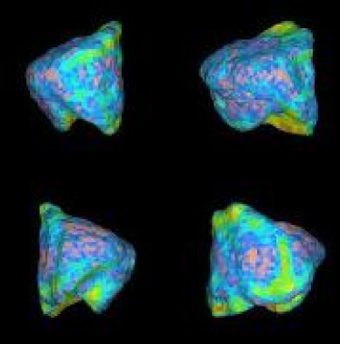
Figure 10: A shape model for the 0.5 km NEA 6489 Golevka derived from Arecibo delay-Doppler images (Hudson et al. 2000; Chesley et al. 2003). The colors indicate the relative size of local gravitational slopes.

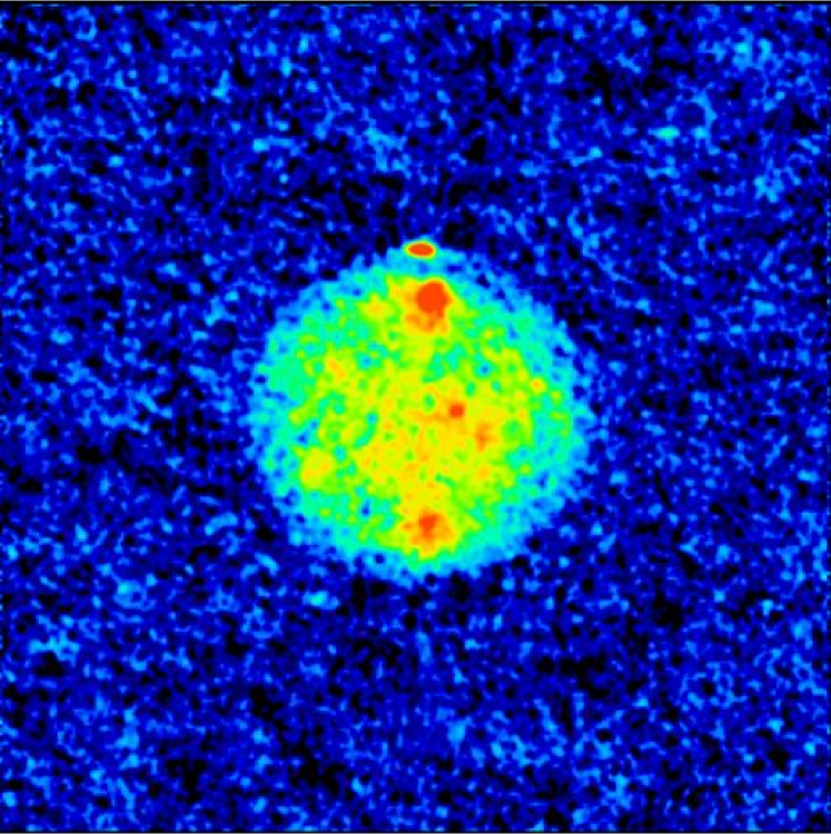
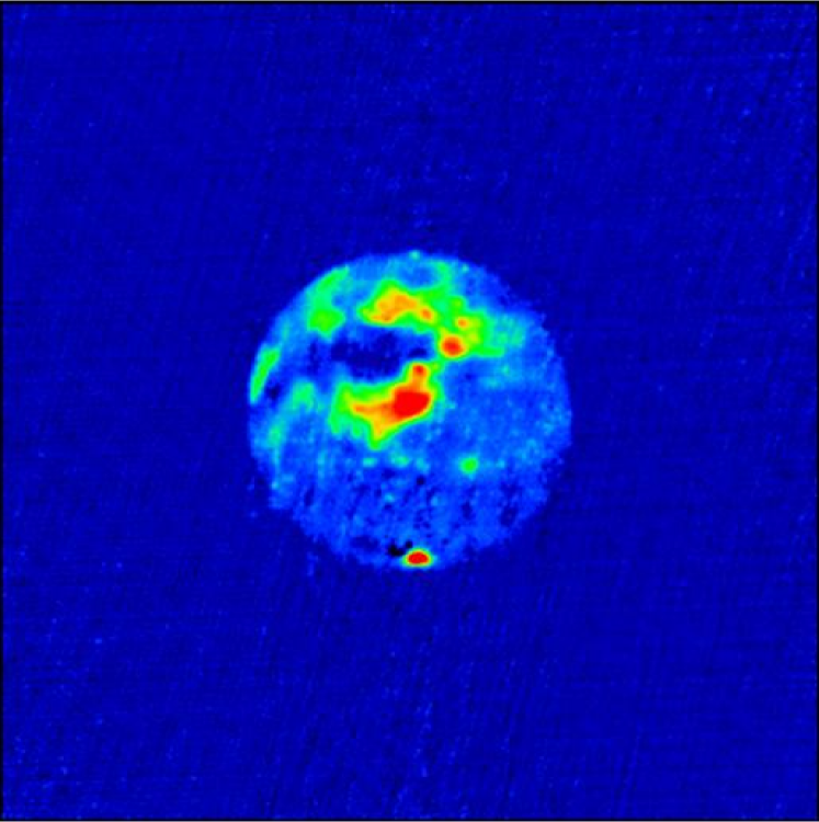
Figure 11: Images made with the combined Goldstone+VLA radar instrument. Mars (left) observations done in October 1988. Mercury (right) observations done in August 1991. In both images, areas of brighter radar reflectivity are red, cycling to lower reflectivity through orange, yellow, green, light blue, blue, purple, and black. After (Muhleman et al. 1991; Butler, Muhleman, & Slade 1993; Muhleman, Grossman, & Butler 1995).

7.1 Terrestrial planets

At the distances of the closest approaches of Mercury, Venus and Mars to the Earth, the spatial resolution of a 3,000 km baseline SKA at 10 GHz will be approximately 1 km, 0.5 km and 0.7 km, respectively. The SKA-based radar system would be capable of imaging the surface of Mercury at 1 km resolution with a 1.0-sigma sensitivity limit corresponding to a radar cross section per unit area of about -30 db, good enough to map to very high incidence angles. For Mars, the equivalent spatial resolution for the same sensitivity limit would be $<$ 1 km. The very high absorption in the Venus atmosphere at 10 GHz would reduce the echo strength and, hence, limit the achievable resolution. However, short wavelength observations would complement the longer 13 cm imagery from Magellan, provide additional information about the electrical properties of the surface via studies of the polarization properties of the echo (Haldemann et al. 1997; Carter, Campbell, & Campbell 2004), and monitor the surface for signs of current volcanic activity. For both Mercury and Mars, radar images at 1 km resolution would potentially be of great interest for studying regolith properties on Mercury and probing the dust that covers much of the surface of Mars. For the polar ice deposits on Mercury the sensitivity would allow sub-km resolution, significantly better than the 2 km Arecibo delay-Doppler imagery of Harmon, Perillat, & Slade (2001). However, this will require the capability to perform delay-Doppler imaging within the SKA’s synthesized beam areas.

7.2 Icy Satellites

Radar is uniquely suited to the study of icy surfaces in the solar system and a SKA based system would provide images (or at least detections) of these bodies in the parameters responsible for their unusual radar scattering properties. As shown by recent Arecibo radar observations of Iapetus, the third largest moon of Saturn, the radar reflection properties of icy bodies can be used to infer surface chemistry in that pure ice surfaces can be distinguished from ones which in- corporate impurities such as ammonia that suppresses the low loss volume scattering properties of the ice (Black et al. 2004) The unusual radar scattering properties of the Galilean satellites have been known for some time (Campbell et al. 1978; Ostro et al. 1992). As such, they are inviting targets for a SKA radar. At a distance to the jovian system of 4.2 AU, the smallest spatial size of the SKAs synthesized beam would be about 6 km while, given the very high backscatter cross sections of the icy Galilean satellites, signal-to-noise considerations would allow imaging with about 5 km resolution, a good match to the size of the synthesized beam. Depending on the prospects for NASAs proposed Jupiter Icy Moons Mission (JIMO) and its instrument payload, radar images of the icy moons at resolutions of a few km would provide unique information about the regoliths/upper surface layers of the icy satellites. Past radar observations of Titan have been instrumental in shaping our ideas of what resides on the surface there - the existence of a deep, global methane/ethane ocean was disproved (Muhleman et al. 1990), but recent Arecibo radar observations have provided evidence for the possible presence of small lakes or seas (Campbell et al. 2003) The Cassini mission, just arriving in the saturnian system, will make radar reflectivity measurements of Titan, but they will not be global, nor will the resolution be as fine as desired. At a distance of 8.0 AU, the spatial resolution of a 3,000 km baseline SKA at 10 GHz will be approximately 12 km - global radar imagery at this scale would be a powerful tool for studying the surface and subsurface of this enigmatic body. Given the extreme sensitivity of the SKA for radar observations, it would even be possible to make detections of Triton and Pluto. At the distances of these bodies, it will probably not be possible to make resolved images of them (although theoretically it is possible, given the SKA resolution) we can still at least measure the bulk properties of their surfaces and make crude hemispherical maps.

A SKA system could also be used to investigate the radar scattering properties of some of the smaller satellites of Jupiter, Saturn and Uranus. It will be possible to investigate the radio wavelength scattering properties of most of the satellites of Jupiter, satellites of Saturn with larger than 50 to 100 km and the five large satellites of Uranus.

7.3 Small bodies

7.3.1 Primary scientific objectives

While spacecraft have imaged a small number of asteroids and comets, Earth based planetary radars will be the dominant means for the foreseeable future for obtaining astrometry, and determining the dynamical state and physical properties of small bodies in the inner solar system. Internal structure and collisional histories, important for solar system formation theories, can be deduced from measurements of asteroid sizes and shapes and from detailed imagery of their surfaces. Variations in the reflection properties of main belt asteroids with distance from the sun could pinpoint the transition region from rocky to icy bodies, again important for theories of solar system formation. There is also considerable uncertainty as to the size distribution of comets that a SKA based radar system could resolve. Bernstein et al. (2004) have pointed out that there is a significant shortage of KBOs at small sizes if comets have nuclei that are in the 10 km range as currently thought.

7.3.2 Near Earth Asteroids

Astrometry and characterization would be major objectives of an SKA based radar system. NEAs are of great interest due to their potential hazard to the Earth, as objectives for future manned space missions to utilize their resources and as clues to the early history of the solar system. Astrometry and measurements of their sizes and spin vectors will greatly reduce the uncertainties in projecting their future orbits including non-gravitational influences such as the Yarkovsky effect (Figure 12). Measurements of the shapes, sizes and densities will provide insights as into the internal structure of NEOs, important both for understanding their history and also for designing mitigation methods should an NEO pose a significant threat to Earth. Unambiguous surface imagery at resolutions of a few meters will give insights into their collisional histories while the polarization properties of the reflected echo can be used to detect the presence of regoliths. Shapes, sizes and surface structure are currently obtained from multiple aspect angle delay-Doppler images (Figure 10 and Hudson 1993). A radar equipped SKA will have the capability to image NEOs out to about 0.3 AU from Earth allowing large numbers to be imaged at resolutions of less than 20 m. The current Arecibo 13 cm radar system has the capability to image NEOs with about 20 m resolution to distances of approximately 0.05 AU. With over 100 times Arecibo’s current sensitivity, an SKA based radar system could achieve similar resolutions at 0.15 to 0.20 AU and much higher resolutions for closer objects. The synthesized beam of the SKA (assuming 3,000 km baseline and 10 GHz frequency) has a spatial resolution at 0.2 AU of about 300 m, very much larger than the achievable resolution based on the sensitivity but small enough to mitigate the effects of delay-Doppler ambiguities allowing improved shape modeling and surface imagery. Doppler discrimination in the synthesis imagery will provide the plane-of-sky direction of the rotation vector (de Pater et al. 1994) and polarization properties will elucidate regolith properties.

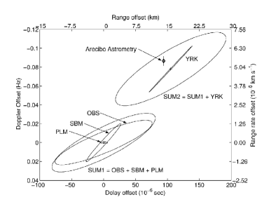
Figure 12: Prediction error ellipses for the location in time delay (distance) and Doppler shift (line-of-sight velocity) of the 0.5 km NEA 6489 Golevka for an Arecibo observation in 2003 based on not including (SUM1) and including (SUM2) the non-gravitational force known as the Yarkovsky effect. The actual measurement indicated by ”Arecibo astrometry” clearly shows that the Yarkovsky effect is important in modifying the orbits of small bodies (from Chesley et al. 2003).

Because of their implications for both the composition and internal structure of asteroids, measurements of densities would be a major objective of SKA observations of NEAs. The discovery of binary NEAs (Figure 13; Margot et al. 2002b) provided the first opportunity for direct measurements of densities for the 10-20% of NEAs that are estimated to be in binary configurations. However, while they provide important information about NEA densities, the primary and secondary components of these binaries are a particular class of NEAs (Margot et al. 2002b) and are not fully representative of the general population. An alternative method of estimating densities for NEAs is the measurement of the Yarkovsky effect via long term astrometric observations (Vokrouhlicky et al. 2004). The size of the effect is dependent on the spin rate, the thermal inertia of the surface and the mass. The first two of these can be measured or estimated allowing the mass to be estimated and, hence, the density if the asteroid s volume is known via a shape model.

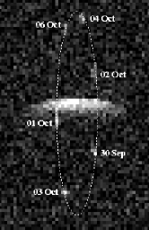
Figure 13: A composite Arecibo delay-Doppler image of the binary near Earth asteroid 2000 DP107 showing the primary body with the location of the secondary on the dates shown in 2000. The diameters of the two bodies are about 800 m and 300 m, the orbital radius and period are 2.6 km and 1.76 days, respectively, giving a density for the primary of approximately 1.7 g cm^-3 (Margot et al. 2002b). Figure courtesy of J.L. Margot.

7.3.3 Main Belt Asteroids

A SKA based radar system would have a unique ability to measure the properties of small bodies out to the far edge of the main asteroid belt; sizes, shapes, albedoes and orbital parameters. The current Arecibo radar system has only been able to obtain a shape model for one MBA, Kleopatra (Figure 14; Ostro et al. 2000) and measure the radio wavelength reflection properties of a relatively small number of asteroids near the inner edge of the belt (Magri et al. 2001) plus those for a few of the very largest MBAs such as Ceres and Vesta (M. Nolan private communication). Main belt issues that a SKA based radar could address are: 1) The size distribution of MBAs would provide valuable constraints on material strength and, hence, on collisional evolution models; 2) Measurement of proportion of MBAs that are in binary systems would provide information about the collisional evolution of the main belt and detection of these systems would also provide masses and densities for a large number of MBAs; 3) Astrometry would also provide masses and densities via measurements of the gravitational perturbation from nearby passes of two bodies and also, for small bodies, from measurements of the Yarkovsky effect; 4) From radar albedo measurements determine whether there is a switch within the main belt from rocky to icy objects and, if so, whether it is gradual or abrupt.

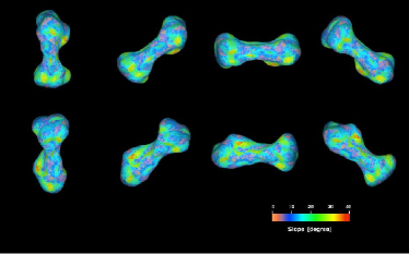
Figure 14: Shape models for the metallic main belt asteroid 216 Kleopatra derived from Arecibo delay-Doppler radar images. The model shows Kleopatra to be 217 km x 94 km x 81 km. It may be the remains of a collision of two former pieces of an ancient asteroids disrupted core. The color coding indicates the gravitational slopes (Ostro et al. 2000).

7.3.4 Comets

Spacecraft flybys have provided reasonable detailed information about three comets, Halley, Borelly and Wild, and over the next 1-2 decades, prior to the completion of the SKA, a small number of additional comets will be studied from spacecraft such as the already launched Deep Impact and Rosetta missions and from potential new missions such as a successor to the failed Contour mission. Direct measurements of the sizes of three comets have indicated that cometary nuclei have very low optical albedoes and this has led to an upward revision of the size estimates of comets based on measurements of their absolute magnitudes. However, the very small sample means that the distribution of cometary albedoes is very uncertain and, hence, there is still considerable uncertainty as to the size distribution of comets. An SKA based radar system could resolve this issue which has ramifications related to the assumed source of short period comets in the Kuiper belt. Bernstein et al. (2004) have pointed out that there is a significant shortage of KBOs at small sizes if comets have nuclei that are in the 10 km range as currently thought. A SKA based radar would be able to image cometary nuclei out to about 1 AU obtaining sizes, shapes, rotation vectors, and actual nucleus surface images. For objects at larger distances, size estimates will be obtained from range dispersion and also from rotation periods from radar light curves combined with measurements of Doppler broadening. Over time these measurements would be the major source of cometary size estimates.

7.4 Technical issues

For many bodies, unambiguous plane-of-sky synthesis imagery is superior to delay-Doppler imagery. Consequently, for both imaging and astrometric observations, a SKA based radar would need to have the capability to do both traditional radar delay-Doppler observations and synthesis imaging of radar illuminated objects. For both range-Doppler imaging and astrometric observations of near earth objects, range resolutions of 20 ns or better will be required. At 10 GHz the angular resolution of even the proposed central compact array will be smaller than the angular size of some NEOs requiring that for delay-Doppler and astrometric observations the SKA will still need to be used in an imaging mode. While adding to the complexity of the observations, the small spatial extent of the synthesized beam will greatly assist in mitigating the ambiguities inherent in delay-Doppler imaging. Delay-Doppler processing will require access to the complex outputs of the correlator at a 20 ns or better sampling rate. This requirement may not be dissimilar from that required for pulsar observations but it will have the added complexity that the NEOs will be in the near field of the SKA.

8 Extrasolar Giant Planets

The detection of extrasolar giant planets is one of the most exciting discoveries of astronomy in the past decade. Despite the power of the radial velocity technique used to find these planets, it is biased to finding planets which are near their primary and orbiting edge-on. To augment those planets found by radial velocity searches, detections using astrometry, which are most sensitive to planets orbiting face-on, are needed. Many researchers are eagerly searching for ways to directly detect these planets, so they can be properly characterized (only the orbit and a lower limit to the mass is known for most extrasolar planets). Below we will discuss potential contributions for SKA.

8.1 Indirect detection by astrometry

The orbit of any planet around its central star causes that star to undergo a reflexive circular motion around the star-planet barycenter. By taking advantage of the incredibly high resolution of SKA, we may be able to detect this motion. Making the usual approximation that the planet mass is small compared to the stellar mass, the stellar orbit projected on the sky is an ellipse with angular semi-major axis $\theta_{r}$ (in arcsec) given by:

$$\theta_{r}={m_{p}\over M_{*}}\,{a_{AU}\over D_{pc}}\quad,$$ (1)

where $m_{p}$ is the mass of the planet, $M_{*}$ is the mass of the star, $a_{AU}$ is the orbital distance of the planet (in AU), and $D_{pc}$ is the distance to the system (in parsecs).

The astrometric resolution of SKA, or the angular scale over which changes can be discriminated ($\Phi$), is proportional to the intrinsic resolution of SKA, and inversely proportional to the signal to noise with which the stellar flux density is detected (${\rm SNR}_{*}$):

$$\Phi={\theta_{HPBW}\over{2\cdot{\rm SNR}_{*}}}\quad.$$ (2)

This relationship provides the key to high precision astrometry: the astrometric accuracy increases both as the intrinsic resolution improves and also as the signal to noise ratio is increased. Astrometry at radio wavelengths routinely achieves absolute astrometric resolutions 100 times finer than the intrinsic resolution, and can achieve up to 1000 times the intrinsic resolution with special care. As long as the phase stability specifications for SKA will allow such astrometric accuracy to be achieved for wide angle astrometry, such accuracies can be reached.

When the astrometric resolution is less than the reflexive orbital motion, that is, when $\Phi\ \lower 1.72218pt\hbox{$\;\buildrel<\over{\scriptstyle\sim}\;$}\ \theta_{r}$, SKA will detect that motion. We use the approximation that $\theta_{HPBW}\sim\lambda/B_{max}$, so that detection will occur when:

$${\rm SNR}_{*}\ \lower 1.72218pt\hbox{$\;\buildrel>\over{\scriptstyle\sim}\;$}\ 10^{5}\,{\lambda\over B_{max}}\left({m_{p}\over M_{*}}\,{a_{AU}\over D_{pc}}\right)^{-1}\quad.$$ (3)

The factor of $2\times 10^{5}$ enters in to convert from radians to arcseconds.

Note, however, that astrometric detection of a planet requires that curvature in the apparent stellar motion be measured, since linear terms in the reflex motion are indistinguishable from ordinary stellar proper motion. This implies that at the very minimum, one needs three observations spaced in time over roughly half of the orbital period of the observed system. A detection of a planetary system with astrometry would thus require some type of periodic monitoring.

We use the technique described in Butler, Wootten, & Brown (2003) to calculate the expected flux density from stars, and whether we can detect their wobble from the presence of giant planets. If all of the detectable stars for SKA (roughly 4300), had planetary companions, how many of them could be detected (via astrometry) with SKA?

We assume that the planets are in orbits with semimajor axis of 5 AU. We consider 3 masses of planetary companions: 5 times jovian, jovian, and neptunian. We assume integration times of 5 minutes, at 22 GHz. From the Hipparcos catalog (Perryman et al. 1997), there are $\sim$ 1000 stars around which a 5*jovian companion could be detected, $\sim$ 620 stars around which a jovian companion could be detected, and $\sim$ 40 stars around which a neptunian companion could be detected. Virtually none of these stars are solar-type. From the Gliese catalog (Gliese & Jahreiss 1988), there are $\sim$ 1430 stars around which a 5*jovian companion could be detected, $\sim$ 400 stars around which a jovian companion could be detected, and $\sim$ 60 stars around which a neptunian companion could be detected. Of these, $\sim$ 130 are solar analogs.

8.2 Direct detection of gyro-cyclotron emission

Detection of the thermal and synchrotron emission from Jupiter, taken to distances of the stars, is beyond even the sensitivity of SKA unless prohibitively large amounts of integration time are spent. However, Jupiter experiences extremely energetic bursts at long wavelengths. If extrasolar giant planets exhibit the same bursting behavior, SKA might be used to detect this emission. If such a detection occurred, it would provide information on the rotation period, strength of the magnetic field, an estimate of the plasma density in the magnetosphere, and possibly the existence of satellites. The presence of a magnetic field is also potentially interesting for astrobiology, since such a field could shield the planet from the harsh stellar environment. Some experiments have already been done to try to detect this emission (Bastian, Dulk, & Leblanc 2000).

These bursts come from keV electrons in the magnetosphere of the planet. The solar wind deposits these electrons, which can subsequently develop an anisotropy in their energy distribution, becoming unstable. When deposited in the auroral zones of the planet, emission results at the gyrofrequency of the magnetic field at the location of the electron ($f_{g}=2.8B_{gauss}$ MHz, for magnetic field strength $B_{gauss}$ in G). This kind of emission occurs on Earth, Saturn, Jupiter, Uranus, and Neptune in our solar system. The emission can be initiated or modulated by the presence of a satellite (Io, in the case of Jupiter).

If we took the mean flux density of Jupiter at 30 MHz ($\sim$ 50000 Jy at 4.5 AU) to 10 pc, the resultant emission would only be 0.2 $\mu$Jy. This is very difficult to detect, given the expected sensitivity of SKA at the lowest frequencies. However, the emission is variable (over two orders of magnitude), some EGPs may have intrinsically more radiated power, and if the emission is beamed, there is a significant increase in the expected flux density.

The details of the expected radiated power from this emission mechanism are outlined in Farrell, Desch, & Zarka (1999) and Zarka et al. (2001). We summarize the discussion here. There exists a very good correlation amongst those planets that emit long wavelength radio waves between radiated power and input kinetic power from the solar wind. Given expressions for the solar wind input power and conversion factor, and a prediction of the magnetic moment of a giant planet, we can write the expected radiated power as:

$$P_{rad}\sim 400\left(\omega\over\omega_{j}\right)^{4\over 5}\left(M\over M_{j}\right)^{4\over 3}\left(d\over d_{j}\right)^{8\over 5}\ [{\rm GW}]\ ,$$ (4)

where $\omega$, $M$, and $d$ are the rotational rate, mass, and distance to primary of the planet, and the subscripted $j$ quantities are those values for Jupiter. The expected received flux density can then be easily calculated, assuming isotropic radiation.

The frequency at which the power is emitted is limited at the high end by the maximum gyrofrequency of the plasma: $f_{g}\sim 2.8B_{gauss}$ [MHz], for magnetic field strength $B_{gauss}$ in G. This usually limits such emissions to the 10’s of MHz (Jupiter’s cutoff is $\sim$40 MHz), but in some cases (for the larger EGPs), can extend into the 100’s of MHz. For this reason, these kinds of experiments might be better done with LOFAR, but there is still a possibility of seeing some of them at the lower end of the SKA frequencies.

If we take the current list of EGPs and use the above formalism to calculate the expected flux density, we can determine which are the best candidates to try to observe gyrocyclotron emission from. In this exercise, we exclude those planets with cutoff frequencies $<$ 10 MHz (Earth’s ionospheric cutoff frequency), and those in the galactic plane (because of confusion and higher background temperature). Table 5 shows the top four candidates, from which it can be seen that the maximum predicted emission is of order a few mJy (note that Farrell, Desch, & Zarka (1999) found similar values despite using slightly different scaling laws). But, again, this is the mean emission, so bursts would be much stronger, and beaming could improve the situation dramatically. Given the multi-beaming capability of SKA, it would be productive to attempt monitoring of some of the best candidates for these kinds of outbursts in an attempt to catch one.

Table 5: Four best candidates for EGP gyrocyclotron emission detection.

Star	$f_{g}$ (MHz)	$F_{r}$ (mJy)
$\tau$ Bootes	42	4.8
Gliese 86	44	2.3
HD 114762	202	0.28
70 Vir	94	0.13

9 The Sun

The Sun is a challenging object for aperture synthesis, especially over a wide frequency range, due to its very wide range of spatial scales (of order 1 degree down to 1^′′), its lack of fine spatial structure below about 1^′′, its great brightness (quiet Sun flux density can be $10^{6}$–$10^{7}$ Jy) and variability (flux density may change by 4-5 orders of magnitude in seconds), and its variety of relevant emission mechanisms (at least three—bremsstrahlung, gyroemission, and plasma emission—occur regularly, and others may occur during bursts). The key to physical interpretation of solar radio emission is the analysis of the brightness temperature spectrum, and because of the solar variability this spectrum must be obtained over relatively short times (less than 1 s for bursts, and of order 10 min for slowly varying quiescent emission). This means that broad parts of the RF spectrum must be observed simultaneously, or else rapid frequency switching must be possible. The Sun produces only circularly polarized emission–any linear component is destroyed due to extreme Faraday rotation during passage through the corona. High precision and sensitivity in circular polarization measurements will be extremely useful in diagnostics of the magnetic field strength and direction.

Through long experience with the VLA and other instruments, it has been found that only antenna spacings less than about 6 km are useful, which corresponds to a synthesized beam of $10^{\prime\prime}/\nu_{\rm GHz}$. This empirical finding agrees with expectations for scattering in the solar atmosphere (Bastian 1994).

Given the specifications of the SKA, some unique solar science can be addressed in niche areas, but only if the system takes account of the demands placed on the instrument as mentioned above. For flares, the system should be designed with an ALC/AGC time constant significantly less than 1 s, should allow for rapid insertion of attenuation, and should allow for rapid frequency switching. There will be little use for the beam-forming (phased array) mode, since even very low sidelobes washing over the Sun will dominate the signal, and there is no way to predict where a small beam should be placed to catch a flare. In synthesis mode, the main advantage of SKA will be in its high sensitivity to low surface brightness variations. The following solar science could be addressed:

9.1 Solar bursts and activity

The Frequency Agile Solar Radiotelescope (FASR) will be designed to do the best possible flare-related science, and it is hard to identify unique science to be addressed by SKA in this area. However, if SKA is placed at a significantly different longitude than FASR, it can cover the Sun at other times and produce useful results. To cover the full Sun, small antennas (of order 2 m above 3 GHz, and 6 m below 3 GHz) are required. Larger antenna sizes, while restricting the field of view, can also be useful when pointed at the most flare-likely active region.

9.2 Quiet sun magnetic fields

The magnetic geometry of the low solar atmosphere governs the coupling between the chromosphere/photosphere and the corona. Hence, it plays an important role in coronal heating, solar activity, and the basic structure of the solar atmosphere. One can uniquely measure the magnetic field through bremsstrahlung emission of the chromosphere and corona, which is circularly polarized due to the temperature gradient in the solar atmosphere. At $\nu\lower 1.72218pt\hbox{$\;\buildrel<\over{\scriptstyle\sim}\;$}10$ GHz, bremsstrahlung is often swamped by gyroemission, but it dominates at higher frequencies over much of the Sun. By measuring the percent polarization $P\%$ and the local brightness temperature spectral slope $n=-\partial\log T_{b}/\partial\log\nu$, one can deduce the longitudinal magnetic field $B_{\ell}=(107/n\lambda)P\%$, with $B_{\ell}$ in G (Gelfreikh 2004). To reach a useful range of field strengths, say 10 G, the polarization must be measured to a precision of about 0.1–0.2% (since $n$ is typically between 1 and 2).

Both FASR and EVLA will address this science area, but FASR’s small (2 m) antennas mean that the complex solar surface will have to be imaged over the entire disk with high polarization precision, while EVLA’s relatively small number of baselines will make imaging at the required precision difficult. If SKA has relatively large antennas (20 m) and high polarization precision, it will be able to add significantly to this important measurement.

9.3 Coronal Mass Ejections

Coronal Mass Ejections (CMEs) are an important type of solar activity that dominates conditions in the interplanetary median and the Sun’s influence on the Earth. Understanding CME initiation and development in the low solar atmosphere is critical to efforts to understand and predict the occurrence of CMEs. It is expected that CMEs can be imaged through their bremsstrahlung emission, but such emission will be of low contrast with the background solar emission. Bastian & Gary (1997) determined that the best contrast should occur near 1 GHz. Although one of the FASR goals is to observe CMEs, the nearly filled aperture and high sensitivity of SKA to low contrast surface brightness variations can make it very sensitive to CMEs. In addition to following the temporal development of the CME morphology, SKA spectral diagnostics can constrain the temperature, density, and perhaps magnetic field within the CME and surrounding structures.

References

- (1)
- Bastian (1994) Bastian, T.S. 1994, ApJ, 426, 774
- Bastian & Gary (1997) Bastian, T.S., & D.E. Gary 1997, JGR, 102, 14031
- Bastian, Dulk, & Leblanc (2000) Bastian, T.S., G.A. Dulk, & Y. Leblanc 2000, ApJ, 545, 1058
- Bernstein et al. (2004) Bernstein, G., et al., 2004, ApJ, accepted
- Berge & Gulkis (1976) Berge, G.L., & S. Gulkis 1976, In: Jupiter, ed T. Gehrels, UofA Press
- Bird et al. (1997) Bird, M.K., W.K. Huchtmeier, P. Gensheimer, T.L. Wilson, P. Janardhan, and C. Lemme 1997, A&A, 325, L5
- Biver et al. (2002) Biver, N., et al., 2002, EM&P, 90, 323
- Black et al. (2004) Black, G.J., D.B. Campbell, L.M. Carter, & S.J. Ostro 2004, Science, 304, 553
- Bolton et al. (2002) Bolton, S.J., et al., 2002, Nature, 415, 987
- Briggs & Sackett (1989) Briggs, F.H., & P.D. Sackett 1989, Icarus, 80, 77
- Brown & Trujillo (2004) Brown, M.E., & C.A. Trujillo 2004, AJ, 127, 2413
- Brown, Trujillo, & Rabinowitz (2004) Brown, M.E., C.A. Trujillo, & D. Rabinowitz 2004, ApJ, in press
- Burns (1992) Burns, J.A. 1992, In: Mars, ed H.H. Kieffer, B.M. Jakosky, C.W. Snyder, & M.S. Matthews, UofA Press
- Butler, Muhleman, & Slade (1993) Butler, B.J., D.O. Muhleman, & M.A. Slade 1993, JGR, 98, 15003
- Butler et al. (1997) Butler, B.J., A.J. Beasley, J.M. Wrobel, & P. Palmer 1997, AJ, 113, 1429
- Butler & Palmer (1997) Butler, B.J., & P. Palmer 1997, BAAS, 29, 1040
- Butler & Gurwell (2001) Butler, B.J., & M.A. Gurwell 2001, In: Science with the Atacama Large Millimeter Array (ALMA), ed A. Wootten, ASP Conference Series, 235
- Butler et al. (2002) Butler, B.J., A. Wootten, P. Palmer, D. Despois, D. Bockelee-Morvan, J. Crovisier, & D. Yeomans 2002, ACM meeting, Berlin
- Butler, Wootten, & Brown (2003) Butler, B.J., A. Wootten, & B. Brown 2003, ALMA Memo 475
- Butler & Sault (2003) Butler, B.J., & R.J. Sault 2003, IAUSS, 1E, 17B
- Campbell et al. (1978) Campbell, D.B., J.F. Chandler, S.J. Ostro, G.H. Pettengill, & I.I. Shapiro 1978, Icarus, 34, 254
- Campbell et al. (2003) Campbell, D.B., G.J. Black, L.M. Carter, & S.J. Ostro 2003, Science, 302, 431
- Carter, Campbell, & Campbell (2004) Carter, L.M., D.B. Campbell, & B.A. Campbell 2004, JGR, 109, E06009
- Cellino, Zappala, & Tedesco (2002) Cellino, A., V. Zappala, & E.F. Tedesco 2002, M&PS, 37, 1965
- Charnley & Rodgers (2002) Charnley, S.B., & S.D. Rodgers 2002, ApJ, 569, L133
- Chesley et al. (2003) Chesley, S.R., et al., 2003, Science, 302, 1739
- Clancy et al. (1992) Clancy, R.T., A.W. Grossman, & D.O. Muhleman 1992, Icarus, 100, 48
- Cooray (2003) Cooray, A. 2003, ApJ, 589, L97
- Cornwell (2004) Cornwell, T., 2004, EVLA Memo 75
- Craddock (1994) Craddock, R.A. 1994, LPSC XXV, 293
- Davis et al. (1979) Davis, D., C. Chapman, R. Greenberg, S. Weidenschilling, & A.W. Harris 1979, In: Asteroids, ed T. Gehrels, UofA Press
- de Pater, Brown, & Dickel (1984) de Pater, I., R.A. Brown, & J.R. Dickel 1984, Icarus, 57, 93
- de Pater & Goertz (1989) de Pater, I., & C.K. Goertz 1989, GRL, 16, 97
- de Pater (1991) de Pater, I. 1991, AJ, 102, 795
- de Pater, Romani, & Atreya (1991) de Pater, I., P.N. Romani, & S.K. Atreya 1991, Icarus, 91, 220
- de Pater, Palmer, & Snyder (1991) de Pater, I., P. Palmer, & L.E. Snyder 1991, In: Comets in the Post-Halley Era, ed R.L. Newburn, Jr. et al., Kluwer
- de Pater & Mitchell (1993) de Pater, I., & D.L. Mitchell 1993, JGR, 98, 5471
- de Pater et al. (1994) de Pater, I., P. Palmer, D.L. Mitchell, S.J. Ostro, & D.K. Yeomans 1994, Icarus, 111, 489
- de Pater, Schulz, & Brecht (1997) de Pater, I., M. Schulz, & S.H. Brecht 1997, JGR, 102, 22043
- de Pater & Sault (1998) de Pater, I., & R.J. Sault 1998, JGR, 103, 19973
- de Pater (1999) de Pater, I. 1999, In: Perspectives in Radio Astronomy: Science with Large Antenna Arrays, ed M.P. van Haarlem, ASTRON Press
- de Pater & Butler (2003) de Pater, I., & B.J. Butler 2003, Icarus, 163, 428
- de Pater & Dunn (2003) de Pater, I., & D.E. Dunn 2003, Icarus, 163, 449
- de Pater et al. (2003) de Pater, I., et al., 2003, Icarus, 163, 434
- de Pater et al. (2004) de Pater, I., D.R. DeBoer, M. Marley, R. Freedman, & R. Young 2004, Icarus, submitted
- DeBoer & Steffes (1996) DeBoer, D.R., & P.G. Steffes 1996, Icarus, 123, 324
- Desch et al. (2002) Desch, S.J., W.J. Borucki, C.T. Russell, & A. Bar-Nun 2002, Rep. Prog. Phys., 65, 955
- Drake (2001) Drake, M. 2001, M&PS, 36, 501
- Dulk et al. (1997) Dulk, G.A., Y. Leblanc, R.J. Sault, H.P. Ladreiter, & J.E.P. Connerney 1997, A&A, 319, 282
- Dunn, de Pater, & Sault (2003) Dunn, D.E., I. de Pater, & R.J. Sault 2003, Icarus, 165, 121
- Dunn, Molnar, & Fix (2002) Dunn, D.E., L.A. Molnar, & J.D. Fix 2002, Icarus, 160, 132
- Edgett et al. (1997) Edgett, K.S., B.J. Butler, J.R. Zimbelman, & V.E. Hamilton 1997, JGR, 102, 21545
- Farrell, Desch, & Zarka (1999) Farrell, W.M., M.D. Desch, & P. Zarka 1999, JGR, 104, 14025
- Fernandez (2002) Fernandez, Y. 2002, EM&P, 89, 3
- Gelfreikh (2004) Gelfreikh, G.B. 2004, In: Solar and Space Weather Radiophysics, eds D.E. Gary & C.O. Keller, Kluwer, in preparation
- Gibbard et al. (1999) Gibbard, S.G., E.H. Levy, J.I. Lunine, & I. de Pater 1999, Icarus, 139, 227
- Gliese & Jahreiss (1988) Gliese, W, & H. Jahreiss 1988, In: Star Catalogues: a Centennial Tribute to A.N. Vyssotsky, ed A.G.D. Philip & A.R. Upgren, L. Davis Press
- Graham et al. (2000) Graham, A.P., B.J. Butler, L. Kogan, P. Palmer, & V. Strelnitski 2000, AJ, 119, 2465
- Grossman, Muhleman, & Berge (1989) Grossman, A.W., D.O. Muhleman, & G.L. Berge 1989, Science, 245, 1211
- Haldemann et al. (1997) Haldemann, A.F.C., D.O. Muhleman, B.J. Butler, & M.A. Slade 1997, Icarus, 128, 398
- Hammel et al. (2004) Hammel, H.B., I. de Pater, S. Gibbard, & G.W. Lockwood 2004, Icarus, in preparation
- Harmon et al. (1999) Harmon, J.K., D.B. Campbell, S.J. Ostro, & M.C. Nolan 1999, P&SS, 47, 1409
- Harmon, Perillat, & Slade (2001) Harmon, J.K., P.J. Perillat, & M.A. Slade 2001, Icarus, 149, 1
- Hirota et al. (1999) Hirota, T., S. Yamamoto, K. Kawaguchi, A. Sakamoto, & N. Ukita 1999, ApJ, 520, 895
- Ho & Townes (1983) Ho, P.T.P., & C.H. Townes 1983, ARA&A, 21, 239
- Hofstadter & Butler (2003) Hofstadter, M.D., & B.J. Butler 2003, Icarus, 165, 168
- Hofstadter & Butler (2004) Hofstadter, M.D., & B.J. Butler 2004, Icarus, in preparation
- Hudson (1993) Hudson, R.S. 1993, Rem. Sens. Rev., 8, 195
- Hudson et al. (2000) Hudson, R.S., et al., 2000, Icarus, 48, 37
- Janssen et al. (2004) Janssen, M.A., M.D. Hofstadter, S. Gulkis, A.P. Ingersoll, M. Allison, S.J. Bolton, & L.W. Kamp 2004, Icarus, submitted
- Jenkins et al. (2002) Jenkins, J.M., M.A. Kolodner, B.J. Butler, S.H. Suleiman, & P.G. Steffes 2002, Icarus, 158, 312
- Jewitt, Aussel, & Evans (2001) Jewitt, D., H. Aussel, & A. Evans 2001, Nature, 411, 446
- Jones (2004) Jones, D.L. 2004, SKA Memo 45
- Leblanc et al. (1997) Leblanc, Y., G.A. Dulk, R.J. Sault, & R.W. Hunstead 1997, A&A, 319, 274
- Magri et al. (2001) Magri, C., G.J. Consolmagno, S.J. Ostro, L.A.M. Benner, & B.R. Beeney 2001, M&PS, 36, 1697
- Margot et al. (1997) Margot, J.L., D.B. Campbell, B.A. Campbell, & B.J. Butler 1997, LPSC, 28, 871
- Margot et al. (2002a) Margot, J.-L., C. Trujillo, M.E. Brown, & F. Bertoldi 2002, BAAS, 34, 871
- Margot et al. (2002b) Margot, J.-L., M.C. Nolan, L.A.M. Benner, S.J. Ostro, R.F. Jurgens, J.D. Giorgini, M.A. Slade, & D.B. Campbell 2002, Science, 296, 1445
- McDonald, Schardt, & Trainor (1980) McDonald, F.B., A.W. Schardt, & J.H.T. Trainor 1980, JGR, 85, 5813
- Mitchel & de Pater (1994) Mitchell, D.L., & I. de Pater 1994, Icarus, 110, 2
- Morbidelli et al. (2002) Morbidelli, A., R. Jedicke, W.F. Bottke, P. Michel, & E.F. Tedesco 2002, Icarus, 158, 329
- Muhleman et al. (1986) Muhleman, D.O., G.L. Berge, D. Rudy, & A.E. Neill 1986, AJ, 92, 1428
- Muhleman et al. (1990) Muhleman, D.O., A.W. Grossman, B.J. Butler, & M.A. Slade 1990, Science, 248, 975
- Muhleman et al. (1991) Muhleman, D.O., B.J. Butler, A.W. Grossman, & M.A. Slade 1991, Science, 253, 1508
- Muhleman & Berge (1991) Muhleman, D.O., & G.L. Berge 1991, Icarus, 92, 263
- Muhleman, Grossman, & Butler (1995) Muhleman, D.O., A.W. Grossman, & B.J. Butler 1995, ARE&PS, 23, 337
- Ostro et al. (1992) Ostro, S.J., et al., 1992, JGR, 97, 18277
- Ostro et al. (2000) Ostro, S.J., et al., 2000, Science, 288, 836
- Perryman et al. (1997) Perryman M.A.C., et al., 1997, A&A, 323, L49
- Rivkin (1997) Rivkin, A. 1997, PhD Thesis, UofA
- Rivkin et al. (2002) Rivkin, A.S., R.H. Brown, D.E. Trilling, J.F. Bell III, & J.H. Plassman 2002, Icarus, 156, 64
- Sault et al. (1997) Sault, R.J., T. Oosterloo, G.A. Dulk, & Y. Leblanc 1997, A&A, 324, 1190
- Sault, Engel, & de Pater (2004) Sault, R.J., C. Engel, & I. de Pater 2004, Icarus, 168, 336
- Schloerb & Gerard (1985) Schloerb, F.P., & E. Gerard 1985, AJ, 90, 1117
- Showman & de Pater (2004) Showman, A., & I. de Pater 2004, Icarus, submitted
- Snyder, Palmer, & de Pater (1989) Snyder, L.E., P. Palmer, & I. de Pater 1989, AJ, 97, 246
- Tedesco et al. (2002) Tedesco, E.F., P.V. Noah, M. Noah, & S.D. Price 2002, AJ, 123, 1056
- van der Tak et al. (1999) van der Tak, F., I. de Pater, A. Silva, & R. Millan 1999, Icarus, 142, 125
- Vokrouhlicky et al. (2004) Vokrouhlicky, D., D. Capek, S.R. Chesley, & S.J. Ostro 2004, Workshop on Asteroid Dynamics, Arecibo Observatory
- Zarka et al. (2001) Zarka, P., R.A. Treumann, B.P. Ryabov, & V.B. Ryabov 2001, Ap&SS, 277, 293