¹Department of Physical Science, Hiroshima University, Higashi-Hiroshima, 739-8526, Japan
²Department of Physics, Kyoto University, Kyoto,739-8502,  Japan
³ ICG, University of Portsmouth, PO12EG, England
⁴Institute of Astronomy and Astrophysics, Academia Sinica, Taipei 106, Taiwan, R.O.C.

Dark energy reflections in the redshift-space quadrupole

Abstract

We show that the redshift-space quadrupole will be a powerful tool for constraining dark energy even if the baryon oscillations are missing from the usual monopole power spectrum and bias is scale- and time-dependent. We calculate the accuracy with which a next-generation galaxy survey based on KAOS will measure the quadrupole power spectrum, which gives the leading anisotropies in the power spectrum in redshift space due to the linear velocity, Finger of God and Alcock-Paczynski effects. Combining the monopole and quadrupole power spectra breaks the degeneracies between the multiple bias parameters and dark energy both in the linear and nonlinear regimes and, in the complete absence of baryon oscillations ($\Omega_{b}=0$), leads to a roughly 500% improvement in constraints on dark energy compared with those from the monopole spectrum alone. As a result the worst case – with no baryon oscillations – has dark energy errors only mildly degraded relative to the ideal case, providing insurance on the robustness of next-generation galaxy survey constraints on dark energy.

Introduction   The promise of next-generation galaxy surveys such as that planned with KAOS (the Kilo-Aperture Optical Spectrograph KAOS ) is to map the distribution of over one million galaxies in the redshift range $z=0.5-3.5$. This redshift coverage will allow the baryon oscillations in the matter power spectrum to be followed as they were stretched by the cosmic expansion, thus providing us with a standard ruler with which to precisely measure the extragalactic distance scale and expansion rate eisen ; Blake ; Linder ; SE ; HH ; Amendola .

However, this technique relies crucially on the assumption that the baryon oscillations will be detected. Although there are tentative indications for this at low-$z$ in the 2df data 2dfosc ; Yamamoto2004 the jury is still out on their existence. If bias turns out to be much more complicated than we think or $\Omega_{b}$ is unexpectedly low we may face an essentially featureless galaxy power spectrum that is too slippery to supply a standard ruler. In that case it is natural to ask whether surveys such as KAOS will yield any constraints on dark energy at all.

The aim of this letter is to show that even in this worst case scenario, next-generation surveys will be able to deliver good constraints on dark energy through a very different route: redshift-space anisotropies and the Alcock-Paczynski (AP) effect Alcock ; BPH ; MS ; MSz ; matubara ; Yamamoto2003 .

In general the power spectrum in redshift space is not isotropic; an effect already seen in the 2df survey Peacock . There is a linear distortion due to the bulk motion of the sources within the linear theory of density perturbation Kaiser , while the Finger of God effect causes radial elongations due to the motion of galaxies in the nonlinear regime PD . In addition there is a geometric distortion due to the AP effect related to the distance-redshift relation of the universe. As a result the redshift-space power spectrum depends on the angle $\theta$ between the line-of-sight direction $\gamma$ and the wave number vector ${{\bf k}}$ (see e.g., SMJMY ).

In general the redshift-space power spectrum can be expanded as TH ; Hamilton :

$$P({\bf k},z)=P(k,\mu,z)=\sum_{l=0,2,4\cdots}P_{l}(k,z){\cal L}_{l}(\mu),$$ (1)

where ${\cal L}_{l}(\mu)$ is the Legendre polynomial, $\mu=\cos\theta$ and $k=|{\bf k}|$. The odd moments vanish by symmetry.

The monopole $P_{0}(k,z)$ represents the angular averaged power spectrum and is usually what we mean by ‘the power spectrum’. At low-z it has been investigated in great depth in the 2df and SDSS surveys. $P_{2}(k,z)$ is the quadrupole spectrum and gives the leading anisotropic contribution. As can be seen in Fig. 1 it will be well-constrained even by just the $z<1.5$ sample, which we label KAOS1 (see Table 1 for definitions). The higher order multipoles are not well-constrained however.

Crucially, the multipole moments reflect different aspects of the redshift distortions in the power spectrum which can therefore aid in breaking degeneracies between the cosmological parameters, bias and dark energy. The purpose of this letter is to consider the extent to which the anisotropic component of the power spectrum, $P_{\ell},~{}\ell\geq 2$, gives new information about dark energy via the nonlinear effects and the geometric (AP) distortion.

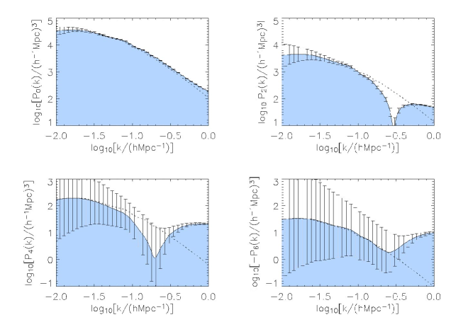
Figure 1: KAOS1 constraints ($z<1.5$) on the multipole moments of the power spectrum, $\langle{\cal P}_{0}(k)\rangle$, $\langle{\cal P}_{2}(k)\rangle$, $\langle{\cal P}_{4}(k)\rangle$ and $\langle{\cal P}_{6}(k)\rangle$ for linear (dotted lines) and nonlinear (shaded region, solid lines) spectra respectively. While the nonlinear correction to ${\cal P}_{0}$ (the usual ‘power spectrum’) is small this is not true for the anisotropic spectra. The nonlinear $\langle{\cal P}_{2}(k)\rangle$ changes sign at large $k$. Here we have fixed $n=1$, $h=0.7$, $\Omega_{b}=0.045$, $\Omega_{m}=0.28$ and $w=-1$. For the bias we adopted $b_{0}=1.35$, $p_{0}=1$ for the linear model, $p_{1}=1$, $b_{1}=0.1$, $\nu=1$ for the nonlinear spectrum (see eq. 7). The higher moments ${\cal P}_{\ell},~{}~{}\ell\geq 4$ are not well-constrained, even by KAOS and hence make a minimal contribution to constraints on dark energy (see Fig.  2).

Formalism   Here we employ the Fisher matrix approach in order to estimate the accuracy with which we can constrain the equation of state, $w\equiv p/\rho$, of the dark energy with a measurement of the power spectrum. In general the Fisher matrix is defined by ${F}_{ij}=-\bigl{\langle}{\partial^{2}\ln L/\partial\theta_{i}\partial\theta_{j}}\bigr{\rangle}$, where $L$ is the likelihood of a data set given the model parameters $\theta_{i}$. Assuming a Gaussian probability distribution function for the errors of a measurement of the multipole power spectrum ${{\cal P}}_{l}(k)$, the Fisher matrix for each multipole spectrum is

$$F_{ij}^{(l)}\simeq{1\over 4\pi}\int_{k_{\rm min}}^{k_{\rm max}}\kappa_{l}(k){\partial\langle{{\cal P}}_{l}(k)\rangle\over\partial\theta_{i}}{\partial\langle{{\cal P}}_{l}(k)\rangle\over\partial\theta_{j}}k^{3}d\ln k,$$ (2)

where $\kappa_{l}(k)$ is the effective volume of the survey available for measuring $\cal P_{\ell}$ at wavenumber $k$:

$$\kappa_{l}(k)^{-1}={1\over 2}\int_{-1}^{1}d\mu{\int d{\bf s}\bar{n}({\bf s})^{4}{\psi}({\bf s},k,\mu)^{4}\bigl{[}P(k,\mu,z)+1/\bar{n}({\bf s})\bigr{]}^{2}[{\cal L}_{l}(\mu)]^{2}\over\Bigl{[}\int d{\bf s}^{\prime}\bar{n}({\bf s}^{\prime})^{2}{\psi}({\bf s}^{\prime},k,\mu)^{2}\Bigr{]}^{2}},$$ (3)

and

$$\langle{{\cal P}}_{l}(k)\rangle={1\over 2}\int_{-1}^{1}d\mu{\int d{\bf s}\bar{n}({\bf s})^{2}{\psi}({\bf s},k,\mu)^{2}P(k,\mu,z){\cal L}_{l}(\mu)\over\int d{\bf s}^{\prime}\bar{n}^{2}({\bf s}^{\prime}){\psi}({\bf s}^{\prime},k,\mu)^{2}},$$ (4)

where ${\psi}({\bf s},k,\mu)$ is a weight factor that we can choose freely, $\bar{n}({\bf s})$ is the mean number density, and ${\bf s}$ denotes the three dimensional coordinate in redshift space. This formula can be derived in a similar way to obtain the optimal weighting scheme (see e.g., FKP ; Yamamoto2003 ). Minimizing the variance on the power spectrum yields ${\psi}({\bf s},k,\mu)=[1+\bar{n}({\bf s})P(k,\mu,z)]^{-1}$, the same as used in SE .

Next we explain our theoretical modelling of the power spectrum. In a redshift survey, the redshift $z$ is the indicator of the distance. Therefore we need to assume a distance-redshift relation $s=|{\bf s}|=s[z]$ to plot a map of objects. The power spectrum depends on this choice of the radial coordinate of the map $s=s[z]$ due to the geometric distortion (AP) effect. For our fiducial background we adopt a flat universe with $\Omega_{m}=0.3$. Here $H_{0}=100~{}h{\rm km/s/Mpc}$ is the Hubble parameter. We consider a cosmological model with the dark energy component with constant equation of state, $w\equiv p/\rho$, since estimates for the nonlinear power spectrum in more general cases do not yet exist. While such an approach has severe limitations when extracting accurate conclusions from real data param , it suffices for our purposes since we are mainly interested in understanding the qualitative improvements in the constraints on $w$ from inclusion of the quadrupole, especially as the baryon oscillations disappear from the monopole.

For constant $w$ we have

$$r(z,\Omega_{m},w)={1\over H_{0}}\int_{0}^{z}{dz^{\prime}\over\sqrt{\Omega_{m}(1+z^{\prime})^{3}+(1-\Omega_{m})(1+z^{\prime})^{-3(1+w)}}}.$$ (5)

Our fiducial model thus has $s(z)\equiv r(z,0.3,-1)$. The geometric distortion in the power spectrum depends on $r(z,\Omega_{m},w)$ and the power spectrum at redshift $z$ is described by scaling the wave numbers from real space to redshift space via $q_{\scriptscriptstyle\|}\rightarrow{k\mu/c_{\scriptscriptstyle\|}}$ and $q_{\scriptscriptstyle\bot}\rightarrow{k\sqrt{1-\mu^{2}}/c_{\scriptscriptstyle\bot}}$ with $c_{\scriptscriptstyle\|}(z)={dr(z)/ds(z)}$ and $c_{\scriptscriptstyle\bot}(z)={r(z)/s(z)}$.

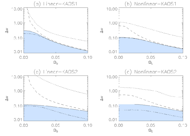
Figure 2: Error estimates for $w$ as the baryon oscillations disappear ($\Omega_{b}\rightarrow 0$). The left panels (a) and (c) are the results using the linear spectrum and the right panels (b) and (d) are the nonlinear spectrum. The dashed curve is the result utilizing only ${\cal P}_{0}(k)$, the dotted curve is the result with only ${\cal P}_{2}(k)$, the solid curve (delimiting the shaded region) is the result obtained using both ${\cal P}_{0}(k)$ and ${\cal P}_{2}(k)$. The target parameters here are same as those in Fig. 1. The low-redshift sample, KAOS1, is assumed in (a) and (b), the high-redshift sample, KAOS2, is assumed in (c) and (d). The dotted-dashed curve in (a) and (b) shows the constraint combining all ${\cal P}_{0}(k)$ to ${\cal P}_{6}(k)$. The double dotted-dashed curve in (c) and (d) shows the constraint obtained from the full KAOS sample (KAOS1 + KAOS2). The key point is how flat the resulting curve is for $\Omega_{b}\leq 0.05$ despite the absence of baryon oscillations for $\Omega_{b}\rightarrow 0$.

We write the galaxy power spectrum in nonlinear theory as

$$P_{\rm gal}(q_{\scriptscriptstyle\|},q_{\scriptscriptstyle\bot},z)=\biggl{(}1+{f(z)\over b(z,q)}{q_{\scriptscriptstyle\|}^{2}\over q^{2}}\biggr{)}^{2}b(z,k)^{2}P^{\rm NL}_{\rm mass}(q,z)D[q_{\scriptscriptstyle\|}],$$ (6)

with $f(z)=d\ln D_{1}(z)/d\ln a(z)$, where $q^{2}=q_{\scriptscriptstyle\|}^{2}+q_{\scriptscriptstyle\bot}^{2}$, $b(z,q)$ is a scale-dependent bias factor, $P^{\rm NL}_{\rm mass}(q,z)$ is the nonlinear mass power spectrum normalized by $\sigma_{8}=0.9$, $D_{1}(z)$ is the linear growth rate, and $a(z)$ is the scale factor. The term in proportion to $f(z)$ describes the linear distortion Kaiser . $D[q_{\scriptscriptstyle\|}]$ represents the damping factor due to the Finger of God effect. Assuming an exponential distribution function for the pair-wise peculiar velocity MJB ; MJS ; SMY gives $D[q_{\scriptscriptstyle\|}]=1/(1+(q_{\scriptscriptstyle\|}\sigma_{P})^{2}/2)$, where $\sigma_{P}$ is the 1-dimensional pair-wise peculiar velocity dispersion estimated in MJB .

For $P^{\rm NL}_{\rm mass}(q,z)$ we adopt the fitting formula for the quintessence cosmological model Ma .

We then use the fitting formula for $f(z)$ developed in WS . For the nonlinear modelling, we assume a four-parameter, scale-dependent, bias model

$$b(z,k)=\left(1+{b_{0}-1\over D_{1}(z)}\right)\left[1+{b_{1}}\left({D_{1}(z)^{p_{1}}q\over 0.1~{}h{\rm Mpc^{-1}}}\right)^{\nu}\right],$$ (7)

where $b_{0}$, $b_{1}$, $p_{1}$ and $\nu$ are the nonlinear bias constants. In the linear case the bias is scale-independent and given by $b(z)=1+(b_{0}-1)D_{1}(z)^{-p_{0}}$ where $p_{0}$ is a constant.

Results   Fig. 1 shows the power spectra $\langle{\cal P}_{0}(k)\rangle$ (usual monopole), $\langle{\cal P}_{2}(k)\rangle$ (quadrupole), $\langle{\cal P}_{4}(k)\rangle$ and $\langle{\cal P}_{6}(k)\rangle$ for the linear and nonlinear models described above, assuming the KAOS1 sample described in Table 1. $\langle{\cal P}_{0}(k)\rangle$ is positive while the nonlinear effects cause $\langle{\cal P}_{2}(k)\rangle$ to change sign at large $k$. For $\langle{\cal P}_{0}(k)\rangle$, the linear power spectrum agrees well with the nonlinear power spectrum because the two nonlinear contributions to it cancel out: the Finger of God effect decreases the amplitude while $P^{\rm NL}_{\rm mass}(k)$ increases the amplitude due to the nonlinearity at large $k$. By comparison, it is very clear that the linear theory is not good for the higher multipole moments on small scales, $k\lower 2.15277pt\hbox{$\;\buildrel>\over{\sim}\;$}0.1h{\rm Mpc}^{-1}$.

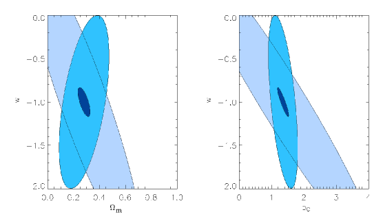
Figure 3: The effect of adding the quadrupole. the $w-\Omega_{m}$ (left) and $w-b_{0}$ (right) likelihoods for ${\cal P}_{0}$ alone (large, medium-blue ellipses), ${\cal P}_{2}$ alone (largest, lightly-shaded ellipses) and ${\cal P}_{0}+{\cal P}_{2}$ (small, darkest ellipses). Here the same parameters are used as in Fig. 1 except that $\Omega_{b}=0$ so there are no baryon oscillations, which explains the poor constraints from ${\cal P}_{0}$ alone. Adding the quadrupole significantly reduces the uncertainty in all the bias parameters resulting in final error ellipses that are competitive with those from the ideal baryon oscillation case, see Fig. 2.

While the quadrupole will make a key contribution to constraining dark energy with KAOS, the errors on $\langle{\cal P}_{4}(k)\rangle$ and $\langle{\cal P}_{6}(k)\rangle$ are large and hence their contribution to constraints on dark energy are marginal, as can be seen from the dot-dashed curves in panel (a) and (b) in Fig. 2.

	KAOS1	KAOS2
redshift range	$0.5<z<1.5$	$2.5<z<3.5$
survey area (deg2)	$103$	$150$
$\bar{n}~{}({\rm h^{3}Mpc^{-3}})$	$10^{-4}$	$10^{-4}$
$k_{\rm max}~{}(h{\rm Mpc}^{-1})$	$0.4$	$1$
$b_{0}$	$1.35$	$1.75$

Table 1: The parameters of the samples used in our analysis. $\bar{n}$ is the average galaxy number density, $k_{\rm max}$ is the maximum wavenumber used in evaluating the Fisher matrix.

The precision with which $w$ can be recovered is shown in Fig 2. We consider separately the low-redshift, $z<1.5$, (KAOS1) and high-redshift (KAOS2) samples, with parameters summarized in Table 1.

To produce these estimates we quote $\Delta w\equiv({\bf F}^{-1/2})_{ww}$, marginalizing over $\Omega_{m}$ and all the bias parameters, viz $b_{0}$, $p_{0}$ (linear case) and $b_{0}$, $p_{1}$, $b_{1}$ and $\nu$ (nonlinear case). Since the bias may be constrained by other methods (e.g. lensing or the higher-order correlation function) our results are conservative.

Fig. 2 shows $\Delta w$ as a function of $\Omega_{b}$. The left panels are the results for the linear perturbation theory, while the right panels are the nonlinear model. The upper panels assume the KAOS1 sample, while the lower panels assume the KAOS2 sample. In general, $\Delta w$ becomes larger as the baryon fraction becomes smaller since the baryon oscillations become less and less distinct. As $\Omega_{b}$ becomes smaller, the contribution from ${\cal P}_{2}$ becomes increasingly important. It is clear from the dashed curve that the constraint on $w$ from ${\cal P}_{0}$ is very weak around $\Omega_{b}=0$ because the baryon oscillations disappear, taking with it the standard ruler. This is the same for the dotted curve which shows the constraints from ${\cal P}_{2}$.

One of the main results of this paper is the solid curve which shows the constraint from the combination of ${\cal P}_{0}$ and ${\cal P}_{2}$. It is good even in the case $\Omega_{b}=0$ when the baryon oscillation are missing, implying that the geometric distortion (AP test) plays the central role in constraining $w$. This does not depends on the bias parameters and inclusion of a constant parameter for stochastic bias does not alter our results TP .

It is interesting to address why the constraint on $w$ from ${\cal P}_{0}$ and ${\cal P}_{2}$ combined is so much better than from either one separately. For each pair of marginalized parameters the error ellipses for ${\cal P}_{0}$ and ${\cal P}_{2}$ are rotated with respect to each other, as in Fig 3, thus breaking degeneracies in the bias-dark energy parameter space. On marginalization these gains are passed through to $w$, resulting in significantly smaller error-ellipses, a feature observed in both the linear and nonlinear cases. The power in combining ${\cal P}_{0}$ and ${\cal P}_{2}$ thus extends the well-known fact that ${\cal P}_{2}$ gives useful information about bias (e.g., TH ; Hamilton ).

Conclusions    We have investigated the accuracy with which we can expect next-generation galaxy surveys such as KAOS KAOS to measure the multipole moments of the anisotropic power spectrum in redshift space and the resulting improvements in dark energy constraints. Anisotropies in the redshift-space power spectrum arise from the contribution of velocities to an object’s redshift as well as from the geometric distortion due to the Alock-Paczynski effect.

We found a number of key results: (1) only the quadrupole among the anisotropic power spectra will be well-measured by KAOS but this is useful for breaking degeneracies between bias and dark energy. (2) Nonlinear effects have a substantial influence on the quadrupole and higher multipoles at scales $k\lower 2.15277pt\hbox{$\;\buildrel>\over{\sim}\;$}0.1h{\rm Mpc}^{-1}$. The inclusion of the nonlinear power spectrum enhances the precision with which the dark energy can be constrained because the nonlinear effects increase the power at small scale which is also where constraints are good. The nonlinear regime provides us with new information about the dark energy, as has been discussed in different contexts (e.g., ND ). (3) Applying these results to dark energy and the KAOS survey we have found that significant constraints arise by combining the monopole and quadrupole spectra even if there are no baryon oscillations in the standard monopole spectrum and even if we allow for multi-parameter scale-dependent or stochastic bias.

This is a key piece of insurance for large galaxy surveys given current uncertainty about the existence of baryon oscillations and ensures that large, next-generation, galaxy surveys will make a significant contribution to the hunt for dark energy irrespective of the existence of baryon oscillations.

Acknowledgements   We thank Daniel Eisenstein and Bob Nichol for comments on the draft. This work is supported by Grant-in-Aid for Scientific Research of Japanese Ministry of Education, Culture, Sports, Science, and Technology 15740155 and by a Royal Society/JSPS Fellowship.

References

- (1) http://www.noao.edu/kaos/
- (2) D. Eisenstein, Proc. WFMOS conference, arXiv:astro-ph/0301623.
- (3) C. Blake, K. Glazebrook, ApJ 594, 665 (2003)
- (4) E. V. Linder, Phys. Rev. D68 083504 (2003)
- (5) H-J Seo, D. J. Eisenstein, ApJ, 598, 720 (2003)
- (6) W. Hu, Z. Haiman, Phys. Rev. D68 063004 (2003)
- (7) L. Amendola, C. Quercellini, E. Giallongo, arXiv:astro-ph/0404599
- (8) C. J. Miller, R. C. Nichol, X. l. Chen, Astrophys. J. 579, 483 (2002)
- (9) K. Yamamoto, ApJ, 605, 620 (2004)
- (10) C. Alcock, B. Paczynski, Nature, 281, 358 (1979)
- (11) T. Matsubara, A. S. Szalay, Phys. Rev. Lett. 90, 021302 (2003)
- (12) W. E. Ballinger, J. A. Peacock, A. F. Heavens, MNRAS, 282, 877 (1996)
- (13) T. Matsubara, Y. Suto, ApJ, 470, L1 (1996)
- (14) T. Matsubara, arXiv:astro-ph/0408349
- (15) K. Yamamoto, ApJ, 595, 577 (2003)
- (16) J. A. Peacock, et al., Nature, 410, 169 (2001)
- (17) N. Kaiser MNRAS, 227, 1 (1987)
- (18) J. A. Peacock, S. J. Dodds, MNRAS, 267, 1020 (1994)
- (19) Y. Suto, H. Magira, Y. P. Jing, T. Matsubara, K. Yamamoto, Prog.Theor.Phys.Suppl. 133, 183, (1999)
- (20) A. N. Taylor, A. J. S. Hamilton, MNRAS, 282, 767 (1996)
- (21) A. J. S. Hamilton, in The Evolving Universe, ed. D. Hamilton, Kluwer Academic, 185 (1998), arXiv:astro-ph/9708102
- (22) H. A. Feldman, N. Kaiser, J. A. Peacock ApJ, 426, 23 (1994)
- (23) B. A. Bassett, P.S. Corasaniti and M. Kunz, astro-ph/0407364 (2004)
- (24) H-J. Mo, Y. P. Jing, G. Boerner, MNRAS, 286 979 (1997)
- (25) Y. Suto, H. Magira, K. Yamamoto, Publ. Astron. Soc. Japan, 52, 249 (2000)
- (26) H. Magira, Y. P. Jing, Y. Suto, ApJ, 528, 30 (1997)
- (27) C-P. Ma, R. R. Caldwell, P. Bode, L. Wang ApJL, 521, L1 (1999)
- (28) L. Wang, P. J. Steinhardt ApJ, 508, 483 (1998)
- (29) M. Tegmark, P. J. E. Peebles, ApJ, 500, L79 (1998)
- (30) J. A. Newman, M. Davis, ApJ, 534, L11 (2000)