The Mass Function and Average Mass-Loss Rate of Dark Matter Subhaloes

Abstract

We present a simple, semi-analytical model to compute the mass functions of dark matter subhaloes. The masses of subhaloes at their time of accretion are obtained from a standard merger tree. During the subsequent evolution, the subhaloes experience mass loss due to the combined effect of dynamical friction, tidal stripping, and tidal heating. Rather than integrating these effects along individual subhalo orbits, we consider the average mass loss rate, where the average is taken over all possible orbital configurations. Under the ansatz that the average distribution of orbits is independent of parent halo mass, this allows us to write the average mass loss rate as a simple function that depends only on redshift and on the instantaneous mass ratio of subhalo and parent halo. After calibrating this model by matching the subhalo mass function (SHMF) of cluster-sized dark matter haloes obtained from high-resolution, numerical simulations, we investigate the predicted mass and redshift dependence of the SHMF. We find that, contrary to previous claims, the subhalo mass function is not universal. Instead, both the slope and the normalization depend on the ratio of the parent halo mass, $M$, and the characteristic non-linear mass $M^{*}$. This simply reflects a halo formation time dependence; more massive parent haloes form later, thus allowing less time for mass loss to operate. We predict that galaxy-sized haloes, with a present-day mass of $M\simeq 10^{12}h^{-1}\>{\rm M_{\odot}}$ have an average mass fraction of dark matter subhaloes that is a factor three lower than for massive clusters with $M\simeq 10^{15}h^{-1}\>{\rm M_{\odot}}$. We also analyze the halo-to-halo scatter in SHMFs, and show that the subhalo mass fraction of individual haloes depends most strongly on their accretion history in the last $\sim 1$ Gyr. Finally we provide a simple fitting function for the average SHMF of a parent halo of any mass at any redshift and for any cosmology, and briefly discuss several implications of our findings.

1 Introduction

During the hierarchical assembly of dark matter haloes, the inner regions of early virialized objects often survive accretion onto a larger system, thus giving rise to a population of subhaloes. This substructure evolves as it is subjected to the forces that try to dissolve it: dynamical friction, tidal forces, and impulsive collisions. Depending on their orbits and their masses, these subhaloes therefore either merge, are disrupted or survive to the present day.

To fully describe, in a statistical sense, the non-linear distribution of mass in the Universe, it is essential that halo substructure is taken into account. After all, galaxies are thought to reside at the centers of dark matter haloes, which includes dark matter subhaloes. When building a coherent picture of galaxy formation or of galaxy clustering, it is therefore of paramount importance that halo substructure is taken into account. In particular, we need an accurate description of the conditional subhalo mass function, $n(m|M){\rm d}m$, which gives the number of subhaloes with masses in the range $m\pm{\rm d}m/2$ that reside in a parent halo of mass $M$. Combined with the (parent) halo mass function, $n(M){\rm d}M$, this then provides a complete, statistical description of the abundance of dark matter haloes down to the level of subhaloes. In addition, a comparison of $n(m|M){\rm d}m$ with the conditional luminosity function, $\Phi(L|M){\rm d}L$ (Yang, Mo & van den Bosch 2003; van den Bosch, Yang & Mo 2003) will yield important insights into galaxy formation and allow for a detailed study of galaxy bias.

Only since a couple of years numerical simulations of structure formation have reached the mass and force resolution to allow for a detailed study of dark matter substructure (e.g., Tormen 1997; Tormen, Diaferio & Syer 1998; Moore et al. 1998, 1999; Klypin et al. 1999a,b; Ghigna et al. 1998, 2000; Stoehr et al. 2002; De Lucia et al. 2004; Diemand, Moore & Stadel 2004; Gill et al. 2004a,b; Gao et al. 2004; Reed et al. 2004; Kravtsov et al. 2004). Most of these studies have found that in terms of their substructure properties, dark matter haloes are homologous; the internal structure of a galaxy-sized halo looks just like a rescaled version of that of a rich cluster. This would imply that the subhalo mass function is independent of parent halo mass. However, most of these results are based on small numbers of individual haloes, while halo-to-halo variations are expected to be fairly large. Combined with uncertainties due to numerical resolution and the identification of dark matter subhaloes, this means that the statistical significance of these results is still unclear. For example, Gao et al. (2004), analyzing a relatively large sample of dark matter haloes extracted from a large, high-resolution simulation, find that the normalization of the SHMF depends on parent halo mass. In particular, they claim that more massive haloes contain a larger mass fraction in subhaloes. Similar results have been obtained by Diemand et al. (2004; their Fig. 7) and Kang et al. (2004; their Fig. 2). Such a parent halo mass dependence might be expected from the fact that more massive haloes form later (e.g., van den Bosch 2002), thus leaving less time for mass loss to operate.

Recently, there have also been a number of analytical studies of dark matter subhaloes based on the extended Press-Schechter (EPS) formalism (Bond et al. 1991; Bower 1991; Lacey & Cole 1993). Although the EPS formalism only yields information regarding parent haloes, it is a logical next step to simply associate the progenitor haloes of a given parent halo (whose properties can be computed using EPS) with its present day subhaloes (Fujita et al. 2002; Sheth 2003). This, however, ignores the fact that subhaloes experience significant amounts of mass loss. A more realistic approach, therefore, needs to combine this EPS based formalism with an analytical description of the (mass) evolution of dark matter subhaloes.

Oguri & Lee (2004), following up on a previous study by Lee (2004), presented a semi-analytical model to compute the SHMF from EPS, taking detailed account of dynamical friction and tidal stripping. They predict that the SHMF is virtually independent of parent halo mass. However, an obvious downside of their approach is that they use the present day mass of the parent halo when computing the impact of dynamical friction. In reality, the parent halo mass evolves, which should have been taken into account (see e.g., Taffoni et al. 2003; Zhao 2004). Therefore, it seems likely that Oguri & Lee have underestimated the impact of dynamical friction, and, since the mass accretion history depends on mass, may not have correctly predicted the mass-dependence of the SHMF. Zentner & Bullock (2003; hereafter ZB03) and Taylor & Babul (2004; hereafter TB04) improve on this by integrating orbits in the changing potential of the parent halo (whose mass accretion history is computed using detailed merger trees). By including detailed analytical descriptions of dynamical friction and tidal heating and stripping, these authors provide detailed, realistic models for the evolution of dark matter substructure. Unfortunately, TB04 refrain from a discussion of predictions regarding the SHMF, while ZB03 only investigate the cosmology-dependence, but not the parent halo mass dependence.

In this paper we follow a similar approach, except that we treat the actual mass loss of subhaloes in a very simple manner. We only consider the average mass loss rate, where the average is considered to be taken over all orbital configurations. This means that we do not have to integrate individual orbits, and allows us to write the mass loss rate as a function of the mass ratio of subhalo to parent halo only. Rather than attempting to obtain an estimate of this average mass loss rate from first principles, we simply adopt a functional form, and adjust the free parameters to match the SHMF obtained from numerical simulations. As in ZB03 and TB04, we take detailed account of the fact that while the subhalo looses mass, the parent halo gains mass due to its hierarchical growth. After calibrating the model against numerical simulations, we use it to investigate the parent halo mass and redshift dependence of the SHMF, as well as the halo-to-halo scatter. We show that our simple model predicts that (i) more massive haloes have a larger mass fraction of substructure, (ii) the halo-to-halo scatter is large, (iii) the abundance of subhaloes per unit parent halo mass is independent of parent mass, and (iv) the subhalo mass fraction is larger at higher redshifts. These findings are in excellent agreement with the numerical simulations of Gao et al. (2004). The main advantage of our model over either numerical simulations or the more detailed models of ZB03 and TB04 is its shear simplicity and computational speed that allows a detailed investigation of the dependence of the SHMF on cosmology, parent halo mass, and redshift. In addition, it provides a simple description of the average mass loss rate of dark matter subhaloes, which may be useful, for example, to describe the evolution of the mass-to-light ratio of satellite galaxies.

This paper is organized as follows. In Section 2 we give a brief overview of the SHMFs obtained from numerical simulations. Section 3 describes our method for computing SHMFs based on a combination of EPS and a simple model for the average mass loss rate of subhaloes. Sections 4, 5, and 6 discuss the mass-dependence, the halo-to-halo variance, and the redshift dependence of the SHMF, respectively. In Section 7 we provide a simple analytical fitting function for the average SHMF of a halo of given mass and redshift. We summarize our results in Section 8.

Throughout we use $m$ and $M$ to denote the masses of the subhalo and the parent halo, respectively. Here the parent halo mass is defined as the total mass (including that of all subhaloes) within a sphere of density 200 times the critical density at redshift zero. For brevity we use $\psi$ to indicate the mass ratio $m/M$, and we consider it understood that $m$, $M$, and $\psi$ all depend on time, without having to write this time-dependence explicitly. A subscript zero is used to indicate the present day value (i.e., at redshift zero). Unless specifically stated otherwise, we adopt a flat $\Lambda$CDM ‘concordance’ cosmology with $\Omega_{m}=0.3$, $\Omega_{\Lambda}=0.7$, $h=H_{0}/(100\>{\rm km}\,{\rm s}^{-1}\,{\rm Mpc}^{-1})=0.7$ and with initial density fluctuations described by a scale-invariant power spectrum with normalization $\sigma_{8}=0.9$.

2 Subhalo Mass Functions from Numerical Simulations

As discussed in the introduction, numerous studies have determined SHMFs from high-resolution numerical simulations. In Fig. 1 we compare the subhalo mass functions from three independent studies (all based on the same $\Lambda$CDM concordance cosmology). The solid dots with errorbars (Poissonian) indicate the average SHMF obtained using the simulations described in Tormen, Moscardini & Yoshida (2004) from 17 clusters with masses in the range $3\times 10^{14}h^{-1}\>{\rm M_{\odot}}\leq M_{0}\leq 1.7\times 10^{15}h^{-1}\>{\rm M_{\odot}}$. These high-resolution simulations were obtained using the technique of re-simulating, at much higher resolution, a region of interest selected from a large cosmological volume. De Lucia et al. (2004) studied a similar set of 11 high resolution re-simulations of galaxy clusters with masses in the range $7\times 10^{13}h^{-1}\>{\rm M_{\odot}}\leq M_{0}\leq 1.8\times 10^{15}h^{-1}\>{\rm M_{\odot}}$. The dashed line in Fig. 1 corresponds to ${\rm d}n/{\rm d}{\rm ln}(m/M)=0.016(m/M)^{-0.94}$, which is the power-law relation that best fits the average SHMF of this set (obtained by fitting their results by eye).. Finally, the solid line indicates the power-law SHMF, ${\rm d}n/{\rm d}{\rm ln}(m/M)=0.017(m/M)^{-0.91}$, that best fits the results of Gao et al. (2004), obtained by fitting-by-eye the average SHMF of their 15 haloes with $3\times 10^{14}h^{-1}\>{\rm M_{\odot}}\leq M_{0}\leq 10^{15}h^{-1}\>{\rm M_{\odot}}$.

All three SHMFs are in good agreement with each other, both in terms of the slope at small $m/M$ and in terms of the normalization. In the range $-3.5\leq{\rm log}(m/M)\leq-2.5$, where the results are most accurate, all three SHMFs agree with each other at better than 20 percent. Given the different force and/or mass resolutions of the various simulations, and the different techniques used to identify subhaloes, this level of agreement is in fact better than what one might naively expect. Especially since relatively small samples of haloes have been used, which, if halo-to-halo scatter is large, may cause significant scatter in these averages. In Section 3.2 below we will use these SHMFs to calibrate our model for the subhalo mass loss rate.

Figure 1: Comparison of SHMFs of parent haloes in the mass range $10^{14}h^{-1}\>{\rm M_{\odot}}\lower 3.01385pt\hbox{$\;\buildrel<\over{\sim}\;$}M_{0}\lower 3.01385pt\hbox{$\;\buildrel<\over{\sim}\;$}10^{15}h^{-1}\>{\rm M_{\odot}}$, as obtained by different authors using different high resolution numerical simulations.

3 Subhalo Mass Functions from Merger Trees

The aim of this paper is to develop an algorithm that allows a fast and reliable computation of subhalo mass functions. As discussed in Section 1 two ingredients are essential: a method to compute progenitor haloes, and a proper treatment of the mass evolution of subhaloes. For the former, we use a standard merger tree, which we construct using the $N$-branch method with accretion (Somerville & Kolatt 1999; hereafter SK99). We adopt the same time-stepping as in SK99, and introduce a lower-mass cut-off of $m_{\rm lim}=10^{-4}M_{0}$, which reflects the effective mass resolution of our merger trees. This cut-off is required since the number of progenitor haloes diverges as the mass goes to zero. Following SK99, any mass contained in haloes below the resolution limit is accounted for by referring to it as ‘accreted’ mass (for which the prior mass accretion history is not followed back in time).

Figure 2: Illustration of the processes of merging and evolution. Each time-step, such as the step between $t=t_{1}$ and $t=t_{2}$ shown here, the parent halo mass grows by merging (assumed instantaneous at $t=t_{1}$), while the subhalo masses evolve due to mass loss. See text for a detailed description.

A proper treatment of the mass evolution of the subhaloes is more complicated. A subhalo moving on a fixed orbit in a static halo experiences mass loss due to tidal stripping and heating. If the orbit were to remain fixed, and in the absence of tidal heating, the mass loss rate would rapidly decline with time, as all mass beyond the tidal radius would be stripped after at most a few orbital periods. In reality, however, tidal heating continues to ‘push’ stars beyond the tidal radius, where they can be stripped, while the orbit evolves due to dynamical friction which causes the tidal radius to shrink. Both effects significantly prolong the duration and increase the amount of mass loss, which may eventually lead to the complete disruption of the subhalo. For detailed numerical simulations of the mass loss of dark matter subhaloes see Hayashi et al. (2003) and Kazantzidis et al. (2004).

To properly account for the above mentioned effects, which depend strongly on the orbital eccentricity (e.g., Colpi, Mayer & Governato 1999; Gnedin, Hernquist & Ostriker 1999; Taylor & Babul 2001, 2004; Taffoni et al. 2003), requires a detailed integration over all individual subhalo orbits. This is complicated by the fact that the mass of the parent halo evolves with time. If the mass growth rate is sufficiently slow, the evolution may be considered an adiabatic process, thus allowing the orbits of subhaloes to be integrated analytically despite the non-static nature of the background potential (this principle is exploited in the models of ZB03 and TB04). In reality, however, haloes grow hierarchically through (major) mergers, making the actual orbital evolution highly non-linear.

In order to sidestep these difficulties, we consider the average mass loss rate of dark matter subhaloes, where the average is to be taken over the entire distribution of orbital configurations. This removes the requirement to actually integrate individual orbits, resulting in a subhalo mass loss rate that depends only on the mass ratio $\psi=m/M$. This is true as long as the average distribution of orbital eccentricities of subhaloes does not depend on parent halo mass. The eccentricity distribution, $P(\epsilon)$, depends on the orbital anisotropy and on the density distribution of the parent halo (van den Bosch et al. 1999). Although more massive haloes are less concentrated on average (Navarro, Frenk & White 1997), which could give rise to a mass dependence of $P(\epsilon)$, van den Bosch et al. (1999) have shown that $P(\epsilon)$ depends much more strongly on the orbital anisotropy than on the actual density distribution of the parent halo. Since there is no obvious reason why the anisotropy of the orbits of subhaloes should depend on halo mass, our assumption that the average, instantaneous mass loss rate of substructure depends only on $m/M$ should be sufficiently accurate.

3.1 The average mass loss rate

During the evolution of the system the parent mass, $M$, will increase due to merging and accretion, whereas the subhalo mass, $m$, will decrease due to the effects discussed above. We postulate that in a steady-state halo, for which $\dot{M}\equiv{\rm d}M/{\rm d}t=0$, the instantaneous, fractional mass loss rate of a dark matter subhalo is given by $\dot{m}/m=f(\psi)$ with $f(x)$ an arbitrary function ($0\leq x\leq 1$), to be determined below. In what follows we assume, for simplicity, that $f(x)$ is well described by a power-law, and write

$$\dot{m}=-{m\over\tau}\,\psi^{\zeta}$$ (1)

Here $\tau$ is a characteristic time scale (in Gyr), and $\zeta$ is an additional free parameter that specifies the mass dependence of the subhalo mass loss rate. The negative sign is to emphasize that $m$ is expected to decrease with time. For a subhalo embedded in a static parent halo ($\dot{M}=0$) this yields

$$m(t)=\left\{\begin{array}[]{ll}m_{i}\,{\rm exp}(-t/\tau)&\mbox{if $\zeta=0$}\\ m_{i}\left[1+\zeta\,\psi_{i}^{\zeta}\,(t/\tau)\right]^{-1/\zeta}&\mbox{otherwise}\end{array}\right.$$ (2)

where we have used the boundary condition $\psi(t=0)\equiv\psi_{i}=m_{i}/M$.

Figure 3: Left-hand panel: The solid histogram indicates the average, evolved SHMF for a parent halo with $M_{0}=10^{15}h^{-1}\>{\rm M_{\odot}}$, obtained from 2000 merger trees with $\tau_{0}=0.13\>{\rm Gyr}$ and $\zeta=0.36$. With these parameters the resulting SHMF best matches those of Gao et al. (2004) and De Lucia et al. (2004), shown as dashed and dot-dashed lines, respectively. Note that the model reveals a high-mass cut-off. The dotted histogram indicates the unevolved SHMF (i.e., without subhalo mass loss) and is shown for comparison. Right-hand panel: Same as left-hand panel, except that here we plot the mass fraction of dark matter subhaloes. Note that ${\rm d}f_{s}/{\rm d}{\rm ln}(m)$ of the evolved subhaloes is very flat, indicating that low mass subhaloes contain a significant fraction of the total subhalo mass.

We emphasize at this stage that the power-law form of the average mass-loss rate has no physical motivation. We choose it purely for simplicity. Note that $\dot{m}$ has to capture the effects of both dynamical friction and tidal stripping. One might therefore expect that the mass loss rates of individual subhaloes differs significantly from the simple power-law form adopted here. However, recall that we use $\dot{m}$ to describe the average mass loss rate, which is not necessarily of the same form as that of individual subhaloes. Furthermore, as we show below, it does seem able to naturally explain the subhalo statistics found in numerical simulations, without the need for a more complicated functional form. Nevertheless, a detailed comparison against the average mass loss rates obtained from numerical simulations is required to check whether our power-law form is truly appropriate.

One naturally expects the characteristic time scale $\tau$ to be related to the dynamical time, $t_{\rm dyn}$, of the parent halo. As shown in Appendix A, in the idealized case of homologous haloes, the mass loss rate of a subhalo on a circular orbit can indeed be written in the form (1) with $\tau=t_{\rm dyn}$. Since $t_{\rm dyn}\propto\rho^{-1/2}$, and since the average density of a dark matter halo is a function of redshift, we thus expect that $\tau=\tau(z)$. The average density of a virialized dark matter halo at redshift $z$ is given by $\bar{\rho}(z)=\Delta_{\rm vir}(z)\,\rho_{\rm crit}(z)$. Here $\rho_{\rm crit}(z)=3H^{2}(z)/8\pi G$ is the critical density for closure, and $\Delta_{\rm vir}(z)$ is a cosmology-dependent quantity for which we use the fitting function of Bryan & Norman (1998). To take proper account of the expected redshift dependence of the characteristic time scale for subhalo mass loss, we write

$$\tau=\tau(z)=\tau_{0}\,\left({\Delta_{\rm vir}(z)\over\Delta_{\rm vir}(0)}\right)^{-1/2}\,\left({H(z)\over H_{0}}\right)^{-1}$$ (3)

with $\tau_{0}$ a free parameter that expresses the characteristic time scale for subhalo mass loss at $z=0$.

Figure 4: Parent halo mass dependence of the SHMF. Upper left-hand panel: Average SHMF for parent haloes of three different masses, as indicated. Less massive parent haloes contain fewer subhaloes at any given mass ratio $m/M$. For comparison, the dot-dashed histogram indicates the unevolved SHMF (which is virtually indistinguishable for parent haloes of different mass). The thin, solid lines are the SHMF fitting functions described in Section 7. Upper right-hand panel: Distributions of the ratio of present day mass to mass at time of accretion, $m_{0}/m(t_{m})$, for all subhaloes in parent haloes with $M_{0}=10^{15}h^{-1}\>{\rm M_{\odot}}$ (solid histogram), $M_{0}=10^{13}h^{-1}\>{\rm M_{\odot}}$ (dashed histogram), and $M_{0}=10^{11}h^{-1}\>{\rm M_{\odot}}$ (dotted histogram). Note that subhaloes in more massive parent haloes have, on average, lost a smaller fraction of their mass. Lower left-hand panel: The average subhalo mass fraction, $\langle f_{s}\rangle$ (averaged over 2000 merger trees), as function of parent halo mass: subhaloes in more massive parent haloes contain a larger mass fraction. Lower right-hand panel: SHMFs scaled per unit parent halo mass. Note that with this scaling, the mass dependence is completely removed (except for the high-mass cut-off, which simply reflects that $m/M<1$). The thin, solid line labelled G04 indicates the results (eq. [6]) obtained by Gao et al. (2004) from high-resolution, numerical simulations, and is in excellent agreement with our model predictions.

3.2 Evolution of the population of subhaloes

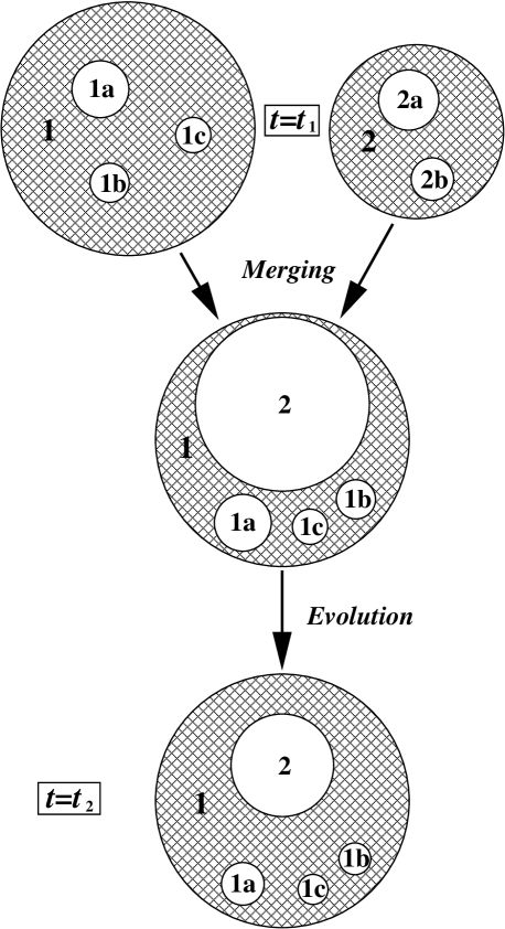
Although the subhalo mass loss rate in a static parent halo is a meaningful concept from a physical point of view, in reality parent haloes themselves evolve due to merging and accretion. In order to take this into account we utilize the discrete time stepping of our merger trees. At the beginning of each time step the parent halo is assumed to increase its mass through (instantaneous) mergers ($\dot{M}>0$, $\dot{m}=0$), while during the period in between two merger events we set $\dot{M}=0$ and evolve $m(t)$ according to eq. (2). The exact procedure is illustrated graphically in Fig 2: At $t=t_{1}$ halo 1 (with three subhaloes) and halo 2 (with two subhaloes) merge. Since $M_{1}>M_{2}$, halo 1 is considered the new parent halo, with halo 2 as a subhalo. In addition, the subhaloes of $M_{1}$ are preserved, and are considered subhaloes of the new, merged halo. The two subhaloes of 2, however, are no longer considered (i.e., we do not follow the evolution of sub-subhaloes). From time $t_{1}$ to $t_{2}$, which is when the next merging or accretion event occurs, the subhaloes evolve according to our mass loss rate, i.e., eq. (2) with $t=t_{2}-t_{1}$, $m_{i}=m(t_{1})$, and $\tau=\tau(t_{1})$. This procedure, hereafter referred to as the ‘Monte-Carlo method’, yields, at each redshift, the evolved SHMF. In addition, we also register for each subhalo the time of merging, $t_{m}$, as well as its mass at that time, $m(t_{m})$. The abundance of these progenitor haloes as function of their mass, $m(t_{m})$, is hereafter referred to as the unevolved SHMF.

In order to calibrate our model, we tune the free parameters $\zeta$ and $\tau_{0}$ such that the SHMF of parent haloes with $M_{0}=10^{15}h^{-1}\>{\rm M_{\odot}}$ matches the subhalo mass functions of Gao et al. (2004) and De Lucia et al. (2004). Although these two SHMFs, obtained from independent numerical simulations, are very similar, the agreement is not perfect. Including the results of Tormen et al. (2004) we estimate the accuracy of the absolute normalization to be about 20 percent, and caution the reader that the absolute normalization of our results is therefore uncertain by a similar amount. Nevertheless, our relative normalizations, which are the main topic of interest here, should not be effected by this. A more robust absolute normalization will have to await a larger sample of high-resolution simulations, and a more detailed investigation of numerical resolution effects.

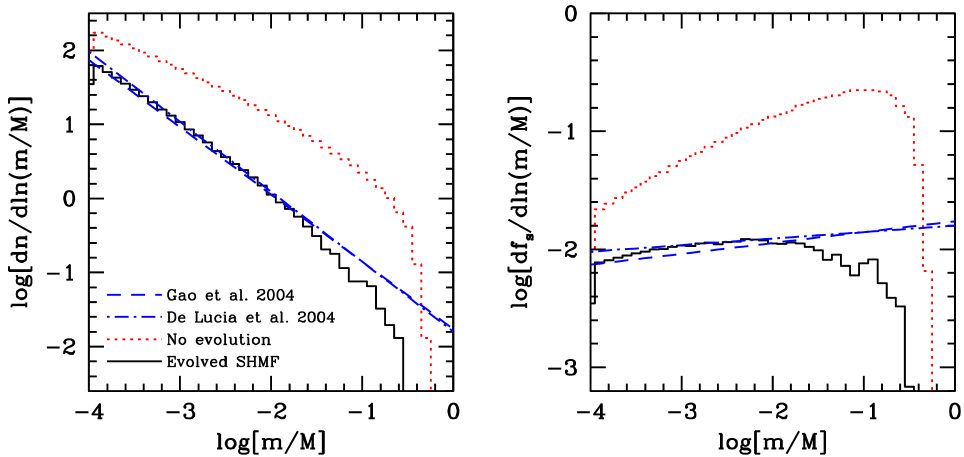
The dotted histogram in the left-hand panel of Fig. 3 plots the average unevolved SHMF obtained from 2000 merger trees for a parent halo of $M_{0}=10^{15}h^{-1}\>{\rm M_{\odot}}$, and is shown for comparison with the evolved SHMF (solid histogram). The latter is obtained from the same 2000 merger trees using the method described above with $\tau_{0}=0.13\>{\rm Gyr}$ and $\zeta=0.36$. These are the parameters for which we obtain the best-fit to the subhalo mass functions of Gao et al. (2004) and De Lucia et al. (2004), shown as dashed and dot-dashed curves, respectively. The agreement with these SHMFs obtained from numerical simulations is very satisfactory, except for a high-mass cut-off in our model, which is not accounted for in the simple power-law fits to the published SHMFs of Gao et al. (2004) and De Lucia et al. (2004). Detailed tests have shown that the location of this high-mass cut-off is robust to changes in $\tau_{0}$ and/or $\zeta$. The former mainly influences the absolute normalization, while the latter controls the slope at small $m/M$.

The right-hand panel of Fig. 3 plots

$${{\rm d}f_{s}\over{\rm d}\,{\rm ln}\,m}=\psi{{\rm d}n\over{\rm d}\,{\rm ln}\,m}$$ (4)

which indicates the mass fraction of the parent halo that is associated with subhaloes of mass $m$. Most of the present day halo mass originates from progenitors (i.e., unevolved subhaloes) with $m(t_{m})\sim 0.1M_{0}$. In fact, if one ignores all progenitors with $m(t_{m})/M_{0}<10^{-4}$ one misses only a negligible fraction of the entire mass. This, however, is not the case for the evolved SHMF. Here ${\rm d}f_{s}/{\rm d}{\rm ln}\,m$ is remarkably flat, indicating that even the evolved subhaloes with $m/M\leq 10^{-4}$ contribute a significant fraction of the total subhalo mass. Therefore, it is important to always indicate the range of $m/M$ considered when quoting subhalo mass fractions, and care is required when comparing subhalo mass fractions from different simulations with different resolutions.

4 The Mass Dependence of the Subhalo Mass Function

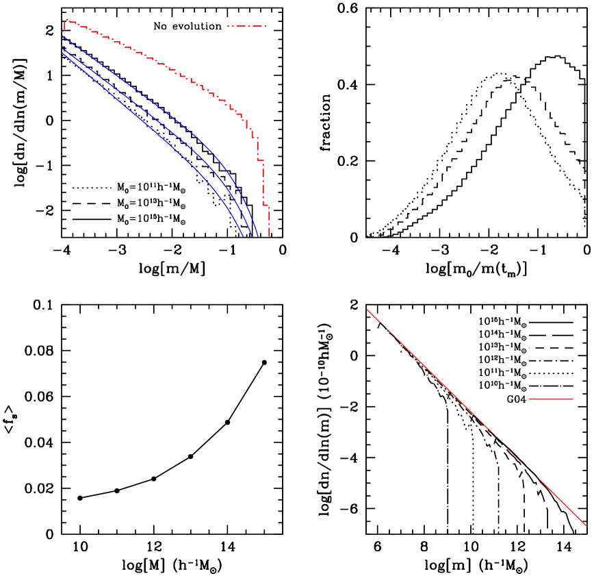
Having calibrated our mass-loss rate by matching the subhalo mass function obtained from numerical simulations for haloes with $M_{0}=10^{15}h^{-1}\>{\rm M_{\odot}}$, we now investigate what the Monte-Carlo method predicts for different parent halo masses. The upper, left-hand panel of Fig. 4 plots the SHMFs obtained using the Monte-Carlo method with $\tau_{0}=0.13\>{\rm Gyr}$ and $\zeta=0.36$ for three different parent halo masses, as indicated (each SHMF is averaged over 2000 merger trees). For comparison, we also show the unevolved subhalo mass function, which is virtually identical for all three halo masses. The evolved SHMFs, however, are clearly mass-dependent with a normalization that decreases systematically with decreasing halo mass. These findings are in good agreement with those of Gao et al. (2004), based on numerical simulation that span three orders of magnitude in parent halo mass, and strongly argue against earlier claims for a universal subhalo mass function (e.g., Moore et al. 1998; De Lucia et al. 2004).

The mass dependence of the normalization of the evolved SHMF is simply a reflection of the fact that less massive haloes form earlier, thus providing more time for mass loss to operate. This is illustrated in the upper, right-hand panel of Fig 4, which plots the distributions of $m_{0}/m(t_{m})$ for parent haloes of $M_{0}=10^{11}h^{-1}\>{\rm M_{\odot}}$ (dotted histogram), $M_{0}=10^{13}h^{-1}\>{\rm M_{\odot}}$ (dashed histogram), and $M_{0}=10^{15}h^{-1}\>{\rm M_{\odot}}$ (solid histogram). These distributions, clearly show that subhaloes in less massive parent haloes have, on average, lost a relatively larger fraction of their mass since they were accreted. The distributions of $m_{0}/m(t_{m})$, however, are very broad; while some subhaloes have only lost a negligible fraction of their initial mass (either because they were accreted relatively late, or because they had small, relative masses to begin with), others have lost more than $99.9$ percent of their mass since their time of accretion.

4.1 The mass fraction in subhaloes

To quantify the mass dependence of the SHMF we consider the mass fraction of dark matter subhaloes with $m\geq 10^{-4}M$:

$$f_{s}\equiv\int_{10^{-4}}^{1}\psi\,{{\rm d}n\over{\rm d}\psi}\,{\rm d}\psi$$ (5)

The lower limit of $10^{-4}$ reflects the effective mass resolution of our merger trees (see Section 3). Throughout this paper all subhalo mass fractions therefore only take account of subhaloes with masses above this resolution limit. As discussed above, the total subhalo mass fraction can easily be a factor two larger than this.

The lower, left-hand panel of Fig. 4 plots $\langle f_{s}\rangle$ at $z=0$ (where the average is taken over 2000 merger trees) as function of parent halo mass. This nicely illustrates the mass dependence of the SHMF indicated above, namely a systematic increase of $\langle f_{s}\rangle$ with increasing parent halo mass. From the scale of galaxy sized haloes ($M_{0}\simeq 10^{12}h^{-1}\>{\rm M_{\odot}}$) to that of massive clusters ($M_{0}\simeq 10^{15}h^{-1}\>{\rm M_{\odot}}$) we find that $\langle f_{s}\rangle$ increases by about a factor three, in reasonable agreement with Gao et al. (2004) and Kang et al. (2004). Note that $\langle f_{s}\rangle(M)$ seems to asymptote to a non-zero value of $\sim 0.01$ for low mass parent haloes, which is simply a reflection of the finite age of the Universe; only in the limit where the formation time of a halo is infinitely long ago will there be sufficient time to wipe out all substructure.

Figure 5: Distributions of $\delta_{f}$ (eq. [7]), obtained from 2000 independent merger trees, for three different parent halo masses as indicated. Note the strong skewness, and the relatively large dispersion. The vertical line indicates the average for which $\delta_{f}=0$. See text for detailed discussion.

4.2 Subhalo mass functions per unit halo mass

The lower, right-hand panel of Fig. 4 shows the subhalo mass functions for six different parent halo masses (each obtained using $\tau_{0}=0.13\>{\rm Gyr}$ and $\zeta=0.36$, and averaged over 2000 merger trees), but this time normalized in a different way. Following Gao et al. (2004) we divide the total number of subhaloes in each bin by the total mass of all the parent haloes (in units of $10^{10}h^{-1}\>{\rm M_{\odot}}$) to obtain the subhalo abundance per unit parent halo mass. These abundances are plotted as function of the actual subhalo mass, $m$, rather than the scaled mass, $m/M$. With this particular normalization, the subhalo mass functions of different parent halo masses agree extremely well (except for the high-mass cut-off). The thin, straight line corresponds to

$${{\rm d}n\over{\rm d}m}=10^{-3.2}\,\left({m\over h^{-1}\>{\rm M_{\odot}}}\right)^{-1.9}h\>{\rm M_{\odot}}^{-1}$$ (6)

which is the best-fit subhalo abundance per unit halo mass (ignoring the high mass cut-off) obtained by Gao et al. (2004). As can be seen, our results are in excellent agreement with those of Gao et al. (2004), lending strong support for our simple model.

Figure 6: Distributions of parent halo formation times, $t_{\rm form}$, (upper left-hand panel) and of the mass fraction $\Delta M(1)/M_{0}$ accreted in the last 1 Gyr (lower left-hand panel). Results are shown for three different parent halo masses, as indicated. The right-hand panels show, for a parent halo mass of $M_{0}=10^{13}h^{-1}\>{\rm M_{\odot}}$, how $t_{\rm form}$ and $\Delta M(1)/M_{0}$ correlate with $\delta_{f}$. The relatively tight relation between $\delta_{f}$ and $\Delta M(1)/M_{0}$ indicates that the subhalo mass fraction of individual haloes depends mainly on their accretion history in the last $\sim 1$ Gyr.

Figure 7: The upper panels plot the distributions $P(N)$, where $N$ is the number of subhaloes with $\log[\psi_{0}]\geq-4$ (upper left panel) and $\log[\psi_{0}]\geq-3$ (upper right panel), respectively. Results, obtained from 2000 merger trees, are shown for three different parent halo masses, as indicated. The lower panels plot $\langle N(N-1)\rangle^{1/2}/\langle N\rangle$ (lower left panel) and $\langle N(N-1)(N-2)\rangle^{1/3}/\langle N\rangle$ (lower right panel), which express the second and third moments of $P(N)$ in the units of that of a Poisson distribution with the same $\langle N\rangle$. See text for a detailed discussion.

5 Scatter in Subhalo Mass Functions

Thus far we only focussed on the average SHMFs, where the average is taken over all orbital configurations and over many mass accretion histories (hereafter MAHs). However, since there is considerable scatter in MAHs of parent haloes of the same mass, and since individual haloes may have significantly different orbital distributions for their subhaloes, one expects a relatively large halo-to-halo variation in the SHMF. Here we use the Monte-Carlo method to obtain an estimate of this scatter. Since this method implicitly averages over all orbital configurations, we can only address the halo-to-halo scatter due to variance in the MAHs. Our estimates of the amount of scatter are therefore to be considered lower-limits.

Fig. 5 plots the distributions of

$$\delta_{f}\equiv{f_{s}-\langle f_{s}\rangle\over\langle f_{s}\rangle}$$ (7)

obtained from 2000 independent MAHs (merger trees). Note that these distributions are extremely skewed (not surprising, given that $f_{s}\geq 0$), and fairly broad. This indicates that the SHMF obtained from a small number of haloes, as is typically the case with current simulations, may not be an accurate representation of the true, average mass function. This explains, at least partially, why it is so difficult to infer from numerical simulations whether or not the SHMF depends on parent halo mass; only when averaged over a sufficiently large number of parent haloes will such a trend become evident.

The upper, left-hand panel of Fig. 6 plots the distributions of the parent halo formation times, $t_{\rm form}$, defined as the lookback time at the redshift where the mass of the most massive progenitor reaches half the present day mass. Although these distributions are very broad, there is a clear mass-dependent trend in that more massive haloes form later. As discussed in Section 4, this explains why $\langle f_{s}\rangle$ increases with parent halo mass; in systems that form later, the subhaloes have less time to experience mass loss. It therefore seems natural that the scatter in $t_{\rm form}$ is the direct source of scatter in $f_{s}$. However, as evident from the upper, right-hand panel of Fig. 6, the correlation between $t_{\rm form}$ and $\delta_{f}$ is, in fact, surprisingly weak.

We find a must stronger correlation between $\delta_{f}$ and $\Delta M(1)/M_{0}$ (lower right-hand panel of Fig. 6), with $\Delta M(1)$ the mass that has been accreted by the parent halo in the last 1 Gyr. This is easy to understand. Since the characteristic time scale for subhalo mass loss is relatively short ($\tau_{0}=0.13$ Gyr) compared to the typical halo formation time, the subhalo mass fraction in individual systems is dominated by the mass that was accreted relatively recently; we find that the scatter between $\delta_{f}$ and $\Delta M(t)/M_{0}$ is minimized for $t\simeq 1.0$ Gyr, which is the value adopted here. A similar conclusion was reached by Gao et al. (2004) who found that subhaloes are typically recent additions to their parent haloes, substantially more recent, in fact, than typical dark matter particles (see also ZB03). Thus, whereas the average SHMF depends strongly on formation time, the SHMF of an individual halo simply reflects its accretion history in the last $\sim 1$ Gyr. Although this may seem contradictory, it is easy to understand when looking at the distributions of $\Delta M(1)/M_{0}$, which are shown in the lower-left panel of Fig 6 for parent haloes of three different masses. As is evident, more massive haloes have, on average, accreted more mass recently, which reflects their relatively later formation times, and which is responsible for the mass-dependence of the average SHMF.

Figure 8: Redshift dependence of the SHMF. Left-hand panel: Subhalo mass functions for parent haloes with a mass of $M(z)=10^{15}h^{-1}\>{\rm M_{\odot}}$ at four different redshifts, as indicated. For comparison, the unevolved SHMF, which is identical for all four cases, is also shown as a dot-dashed histogram. Note that haloes at high redshift contain, on average, more subhaloes than haloes of of the same mass at lower redshifts. As in Fig. 4 the thin, solid lines are the SHMF fitting functions described in Section 7. Right-hand panel: Redshift dependence of the average subhalo mass fraction, $\langle f_{s}\rangle$, for parent haloes of 5 different masses. Each curve is labelled by $M(z)$ (in $h^{-1}\>{\rm M_{\odot}}$).

In addition to the scatter in the subhalo mass fraction $f_{s}$, we also investigate the scatter in the number of subhaloes. The upper two panels of Fig. 7 plot the distributions $P(N)$, where $N$ is the number of subhaloes with $\log[\psi_{0}]\geq-4$ (upper left panel) and $\log[\psi_{0}]\geq-3$ (upper right panel), respectively. Results are shown for three different parent halo masses, as indicated. As above, these probability distributions reflect 2000 independent MAHs (per parent halo mass). These two panels, once again, clearly demonstrate that the subhalo mass function is not universal, but instead depends strongly on parent halo mass: more massive haloes contain more subhaloes above a give $\psi$-threshold. The lower two panels plot ${\cal M}_{2}\equiv\langle N(N-1)\rangle^{1/2}/\langle N\rangle$, related to the second moment, and ${\cal M}_{3}\equiv\langle N(N-1)(N-2)\rangle^{1/3}/\langle N\rangle$, related to the third moment, of these distributions, as function of parent halo mass $M$. Note that for a Poissonian distribution ${\cal M}_{2}={\cal M}_{3}=1$, while distributions that are narrower (sub-Poissonian) or broader (super-Poissonian) have ${\cal M}<1$ and ${\cal M}>1$, respectively. Clearly, when considering all subhaloes with $\log[\psi_{0}]\geq-4$ (solid lines), the $P(N)$ are very close to Poissonian. However, when only counting the more massive subhaloes, with $\log[\psi_{0}]\geq-3$, the distributions are super-Poissonian, with a clear trend of increasing ${\cal M}$ with decreasing parent halo mass. These results are inconsistent with Kravtsov et al. (2004), who finds that the number of subhaloes in numerical simulations follow Poisson statistics. This may reflect a generic problem of the EPS formalism used here to construct the merger trees: as shown by various authors (Lacey & Cole 1993; Somerville et al. 2000; van den Bosch 2002; Wechsler et al. 2002), the halo formation times predicted by EPS are systematically offset from those obtained from numerical simulations. In particular, Somerville et al. (2000) found the average mass of the largest progenitor to be larger with the EPS formalism than in the simulations. This may explain why we find the non-Poissonian nature of $P(N)$ to be more pronounced for more massive subhaloes. Although the merger trees extracted from numerical simulations have their own problems, we caution that the scatter issues discussed here are probably less reliable than the average mass trends.

6 Redshift evolution of the Subhalo Mass Function

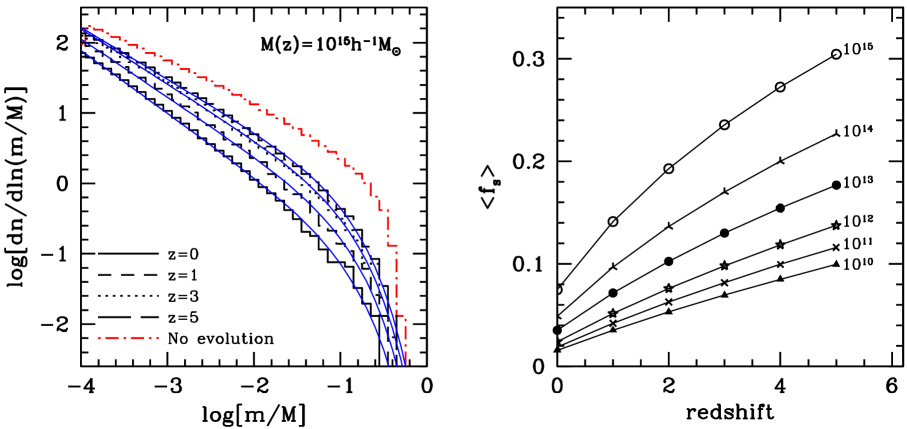
The left-hand panel of Fig. 8 shows the average subhalo mass functions for parent haloes of the same mass, $M(z)=10^{15}h^{-1}\>{\rm M_{\odot}}$, but at different redshifts. At higher redshifts parent haloes of the same mass have a larger abundance of subhaloes than their counterparts at lower redshifts. This is quantified more clearly in the right-hand panel of Fig. 8, which shows the redshift dependence of the average subhalo mass fraction. The various curves are labelled by the parent halo mass $M(z)$ (in $h^{-1}\>{\rm M_{\odot}}$). In all cases $\langle f_{s}\rangle(z)$ increases with redshift, though with a rate, ${\rm d}\langle f_{s}\rangle/{\rm d}z$, that decreases monotonically. Roughly speaking, the subhalo mass fraction at $z=1$ is about twice as large as that of a halo with the same mass at $z=0$.

Figure 9: The dependence of $\langle f_{s}\rangle$ (top panel), $\alpha$ (middle panel), and $\beta$ (bottom panel) on the mass ratio $M/M^{*}$. Solid and open circles correspond to parent haloes in a $\Lambda$CDM concordance cosmology and a SCDM cosmology, respectively. Both the normalization and the shape parameters $\alpha$ and $\beta$ are tightly correlated with $M/M^{*}$, indicating that the latter is the main parameter determining the average SHMF of dark matter haloes. The solid lines are the best-fit functions (9), (13), and $\beta=0.13$ discussed in the text.

The subhalo mass fraction of a given halo at redshift $z$ is a trade-off between the time scale, $t_{\rm acc}$, on which new subhaloes are being ‘accreted’ by the parent halo, and the time scale, $\tau$, of subhalo mass loss. The latter evolves with redshift as described by eq. (3), and therefore was shorter in the past. The former depends on the detailed MAH, and is thus a function of both redshift and parent halo mass. In the limit where $t_{\rm acc}\ll\tau$, subhalo mass loss is negligible and $f_{s}$ will increase with time. The opposite limit, in which $t_{\rm acc}\gg\tau$, is equivalent to that of subhalo mass loss in a static parent halo. In this case, $f_{s}$ will decrease with time. Since the subhalo mass fraction always decreases with time, the time scale for subhalo mass loss is always smaller than that of mass accretion; $\tau<t_{\rm acc}$.

7 An analytical fitting function for the subhalo mass function

Since the unevolved SHMF is virtually independent of $M$, $z$, or even of the cosmological parameters (see Lacey & Cole 1993 and ZB03 for detailed discussions), and since we have adopted a universal, average subhalo mass loss rate, the average, evolved SHMF simply depends on the halo formation time. This suggests that the mass, redshift, and cosmology dependence of the average SHMF can be written as a simple one-parameter dependency on the mass ratio $M/M^{*}$, with the characteristic non-linear mass $M^{*}(z)$ defined by $\sigma(M^{*},z)=\delta_{c}(z)$. Here $\sigma^{2}(M,z)$ is the mass variance of the smoothed density field at redshift $z$ and

$$\delta_{c}(z)=0.15\,(12\pi)^{2/3}\,[\Omega_{m}(z)]^{0.0055}$$ (8)

is the critical threshold for spherical collapse (e.g., Navarro et al. 1997).

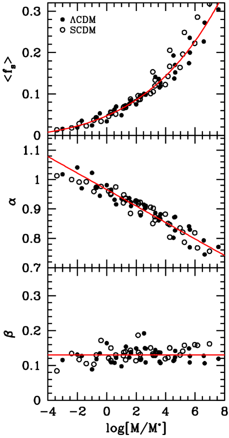
The top panel of Fig. 9 plots the average subhalo mass fraction, $\langle f_{s}\rangle$, as function of $M/M^{*}$ (solid circles). Results are shown for six different parent halo masses (${\rm log}[M/h^{-1}\>{\rm M_{\odot}}]=10,11,...,15$) at six different redshifts ($z=0,1,..5$). Although this yields values of $M/M^{*}$ up to $10^{8}$, we caution that systems with $M/M^{*}\lower 3.01385pt\hbox{$\;\buildrel>\over{\sim}\;$}10^{4}$ are extremely rare. The open circles indicate the results for the same halo masses and redshifts, but obtained for a SCDM cosmology with $\Omega_{m}=1.0$, $\Omega_{\Lambda}=0.0$, $h=0.5$, and $\sigma_{8}=0.7$. All these different haloes follow a tight relation between $\langle f_{s}\rangle$ and $M/M^{*}$, which is well fitted by

$${\rm log}[\langle f_{s}\rangle]=\sqrt{0.4({\rm log}[M/M^{*}]+5)}-2.74$$ (9)

indicated by the solid line. This indicates that, as expected, the average subhalo mass function is completely specified by the mass ratio $M/M^{*}$. To quantify this further we fit the average subhalo mass functions with a Schechter function of the form

$${{\rm d}n\over{\rm d}{\rm ln}\psi}={\gamma\over\beta\,\Gamma(1-\alpha)}\left({\psi\over\beta}\right)^{-\alpha}\,{\rm exp}\left(-{\psi\over\beta}\right)$$ (10)

(cf. Vale & Ostriker 2004). Here $\beta M$ is a characteristic mass, such that for $m\gg\beta M$ the SHMF reveals an exponential decline, and $\gamma$ is the total subhalo mass fraction, i.e.,

$$\gamma=\int_{0}^{\infty}\psi\,{{\rm d}n\over{\rm d}\psi}\,{\rm d}\psi$$ (11)

Some of these fits are shown as thin, solid lines in Fig. 4 (upper left-hand panel) and Fig. 8 (left-hand panel), and in general match the model SHMFs extremely well. Note that in practice we don’t fit the actual SHMF, ${\rm d}n/{\rm d}{\rm ln}\psi$, but rather the corresponding ${\rm d}f_{s}/{\rm d}{\rm ln}\psi$, treating $\alpha$ and $\beta$ as free parameters. The normalization, $\gamma$, is not treated as a free parameter, but is fixed by requiring to match the subhalo mass fraction $f_{s}$, which implies

$$\gamma={f_{s}\over P(1-\alpha,1/\beta)-P(1-\alpha,10^{-4}/\beta)}$$ (12)

with $P(a,x)$ the incomplete Gamma function.

The middle and bottom panels of Fig. 9 plot the best-fit $\alpha$ and $\beta$ for each of the 72 SHMFs (2 cosmologies, 6 masses, 6 redshifts) as function of the mass ratio $M/M^{*}$. As with the average subhalo mass fraction, $\alpha$ and $\beta$ are both tightly correlated with the parent halo mass in units of the characteristic non-linear mass; the power-law slope $\alpha$ scales roughly linearly with ${\rm log}(M/M^{*})$, which is best fit by

$$\alpha=0.966-0.028\,{\rm log}(M/M^{*})\,,$$ (13)

while the parameter $\beta$ is best fit by $\beta=0.13$.

We thus have obtained an extremely simple recipe to compute the average subhalo mass function for a parent halo of any mass, at any redshift, and for any cosmology: compute the characteristic non-linear mass $M^{*}(z)$, and use eq. (9) and (13) to obtain both $f_{s}$ and $\alpha$. The normalization $\gamma$ then follows from (12), which, together with $\beta=0.13$, completely specifies the SHMF.

8 Conclusions

We combined merger trees of dark matter haloes, constructed using the EPS formalism, with a simple prescription of the average mass loss rate of dark matter subhaloes, to compute subhalo mass functions. We calibrated the subhalo mass loss rate by matching the SHMFs of massive haloes with $M_{0}=10^{15}h^{-1}\>{\rm M_{\odot}}$ obtained from high-resolution, numerical simulations. Under the assumption that this average mass-loss rate only depends on redshift and on the mass ratio of sub- and parent halo, $m/M$, this method allows us to make detailed predictions for the mass and redshift dependence of the SHMF, and to investigate the halo-to-halo variance.

Our main conclusions are:

• Contrary to previous claims, the subhalo mass function is not universal. Instead, both the slope and the normalization depend on the ratio of parent halo mass, $M$, to characteristic non-linear mass, $M^{*}$. This simply reflects a halo formation time dependence, in which parent haloes that form earlier have a lower subhalo mass fraction, because there is relatively more time for subhalo mass loss to operate.

• When the subhalo mass function is normalized by the mass of the parent halo, the abundance of subhaloes is universal, in excellent agreement with the numerical simulations of Gao et al. (2004) and Kravtsov et al. (2004).

• The subhalo mass function of an individual halo depends most strongly on its accretion history in the last $\sim 1$ Gyr. This indicates, as previously shown by ZB03 and Gao et al. (2004), that the population of the more massive dark matter subhaloes is, at any time, relatively young.

• The dependence of SHMF on the recent accretion history introduces a large halo-to-halo scatter in the SHMFs, with a distribution of subhalo mass fractions that is strongly skewed towards large values.

• The average subhalo mass function of dark matter haloes is a one-parameter family, depending only on the mass ratio $M/M^{*}$. We have provided simply fitting functions that allow one to compute the average SHMF for a parent halo of any mass, at any redshift, and for any cosmology.

While this paper was being refereed, a paper appeared by Zentner et al. (2004) which uses a similar semi-analytical model as in ZB03 and TB04 to compute subhalo statistics. Using a proper integration of individual orbits, and taking detailed account of dynamical friction and tidal stripping, these authors reach conclusions that are in excellent agreement with the simplified method presented here. In particular, they find that (i) the subhalo mass function is not universal but scales with halo mass, (ii) the subhalo mass function is most sensitive to the most recent accretion history of the parent halo, and (iii) the distribution of the number of subhaloes per parent halo is super-Poissonian. The good agreement of this more sophisticated model with that presented here, provides further support for our ‘orbit averaged’ approach.

These results have a number of important, astrophysical implications. For example, the prediction that the average subhalo mass fraction in galaxy sized haloes is a factor three lower than in cluster-sized haloes has important implications for the magnitude of the claimed substructure crisis (Moore et al. 1999; Klypin et al. 1999b: D’Onghia & Lake 2004), for the flux-ratio statistics of multiply lensed quasars (e.g., Chiba 2002; Metcalf & Madau 2001; Bradač et al. 2002; Dalal & Kochanek 2002), and for the build-up of the galactic halo (Helmi, White & Springel 2003). Furthermore, the redshift dependence of the subhalo mass fraction impacts on the survival probability of fragile structures in dark matter haloes, such as tidal streams and/or galactic disks (Tóth & Ostriker 1992; Taylor & Babul 1991). The subhalo mass functions derived here may also be used in combination with the so-called halo model (see Cooray & Sheth 2002 and references therein) to give a full statistical description of the distribution of dark matter haloes down to the level of subhaloes. This will proof especially fruitful in combination with the conditional luminosity function formalism developed by Yang et al. (2003) and van den Bosch et al. (2003), allowing for a detailed, statistical description of the relation between light and mass (see also Vale & Ostriker 2004). Finally, the average mass loss rates derived here may proof useful in semi-analytical models for galaxy formation, where a proper treatment of the evolution of subhaloes is extremely important (Springel et al. 2002; Benson et al. 2002; Kang et al. 2004).

Finally we point out that, although the Monte-Carlo method presented here is nice and simple, it is important to be aware of its potential shortcomings. For example, the accuracy of the absolute normalization of our model is only as good as that of the SHMFs used for its calibration, which we estimate to be about $\sim 20$ percent. In the numerical simulations used for this calibration, the masses of the parent haloes are defined as the masses within a sphere of density 200 times the critical density at redshift zero. Therefore, we have implicitly assumed that the masses in the EPS formalism used to construct our merger trees are defined in the same way. Since it is still unclear what the proper interpretation of these EPS masses is (see White 2002 for a detailed discussion), this ‘definition’ may introduce an additional uncertainty in the absolute normalization of our results. The fact that the method to construct merger trees is not without its own shortcomings (e.g., SK99; TB04; Sheth & Tormen 1999; Benson, Kamionkowski & Hassani 2004) may have additional implications for the accuracy of our results. Furthermore, we have ignored the weak dependence of halo concentration on halo mass, which may cause a (weak) dependence of the average subhalo mass loss rate on $M$ in addition to $\psi$ (see e.g., ZB03). Finally, we have ignored any possible effect due to subhalo-subhalo mergers. Although the excellent agreement between our results and those of Gao et al. (2004) suggest that none of these effects have a strong impact, large, high-resolution numerical simulations are required to further test both the validity of our approach as well as the accuracy of our results.

Appendix A The Mass loss rate of subhaloes on circular orbits

Consider a subhalo with density distribution $\rho_{s}(r)$ on a circular orbit in a parent halo with density distribution $\rho_{p}(r)$. For simplicity, we assume that both $\rho_{s}(r)$ and $\rho_{p}(r)$ are singular, isothermal spheres.

In the absence of tidal heating, the mass loss rate of the subhalo is given by

$${{\rm d}m\over{\rm d}t}={{\rm d}m\over{\rm d}r_{\rm tid}}\,{{\rm d}r_{\rm tid}\over{\rm d}t}$$ (14)

with $r_{\rm tid}$ the instantaneous tidal radius of the subhalo. We define this tidal radius as the radius of the subhalo where its density is equal to that of the parent halo at the orbital radius $r_{\rm orb}$ of the satellite: $\rho_{s}(r_{\rm tid})=\rho_{p}(r_{\rm orb})$. Since $\rho_{s}(r)$ and $\rho_{p}(r)$ are scale-free we have that

$${1\over r_{\rm tid}}\,{{\rm d}r_{\rm tid}\over{\rm d}t}={1\over r_{\rm orb}}\,{{\rm d}r_{\rm orb}\over{\rm d}t}$$ (15)

The evolution of $r_{\rm orb}$ is governed by dynamical friction, and is given by

$${{\rm d}r_{\rm orb}\over{\rm d}t}=-0.428\,{G\,m\over V_{c}\,r_{\rm orb}}\,{\rm ln}\Lambda$$ (16)

(Binney & Tremaine 1987) with $V_{c}$ the circular velocity of the parent halo and ${\rm ln}\Lambda$ the Coulomb logarithm, which, to leading order, is just a function of the mass ratio $m/M$ (Binney & Tremaine 1987).

Using that ${\rm d}m/{\rm d}r_{\rm tid}=4\pi\rho_{s}(r_{\rm tid})\,r_{\rm tid}^{2}$ and $V^{2}_{c}=GM/r_{\rm vir}$, with $r_{\rm vir}$ the virial radius of the parent halo, we obtain that

$${{\rm d}m\over{\rm d}t}\propto-\rho_{s}(r_{\rm tid})\,V_{c}\,{r_{\rm tid}^{3}\,r_{\rm vir}\over r^{2}_{\rm orb}}\,{m\over M}\,{\rm ln}\Lambda$$ (17)

Defining the dynamical time as $t_{\rm dyn}\propto r_{\rm vir}/V_{c}$ and using that $m\propto\rho_{s}(r_{\rm tid})r_{\rm tid}^{3}$, the subhalo mass loss rate can be written as

$${{\rm d}m\over{\rm d}t}\propto-{m\over t_{\rm dyn}}\,\left({r_{\rm vir}\over r_{\rm orb}}\right)^{2}\,{m\over M}\,{\rm ln}\Lambda$$ (18)

Therefore, when averaging over all possible circular orbits, i.e., all possible ratios $r_{\rm vir}/r_{\rm orb}$, one obtains an average mass loss rate for which

$${{\rm d}m\over{\rm d}t}\propto-{m\over t_{\rm dyn}}\,g(m/M)$$ (19)

with $g(x)$ an arbitrary function. This is the basic form for the average mass loss rate adopted in this paper. Note that since $t_{\rm dyn}\propto\rho^{-1/2}$, and since the average density of dark matter haloes change with redshift, eq. (19) automatically implies a redshift dependence (see Section 3.1).

References

- [] Benson A.J., Lacey C.G., Baugh C.M., Cole S., Frenk C.S., 2002, MNRAS, 333, 156
- [] Benson A.J., Kamionkowski M., Hassani S.H., 2004, preprint (astro-ph/0407136)
- [] Binney J.J., Tremaine S.D., 1987, Galactic Dynamics. (Princeton: Princeton University Press)
- [] Bond J.R., Cole S., Efstathiou G., Kaiser N., 1991, ApJ, 379, 440
- [] Bower R.G., 1991, MNRAS, 248, 332
- [] Bradač M., Schneider P., Steinmetz M., Lombardi M., King L.J., Porcas R., 2002, A&A, 388, 373
- [] Bryan G., Norman M., 1998, ApJ, 495, 80
- [] Chiba M., 2002, ApJ, 565, 17
- [] Colpi M., Mayer L., Governato F., 1999, ApJ, 525, 720
- [] Cooray A., Sheth R.K., 2002, Phys. Reports, 372, 1
- [] Dalal N., Kochanek C.S., 2002, ApJ, 572, 25
- [] De Lucia G., et al., 2004, MNRAS, 348, 333
- [] Diemand J., Moore B., Stadel J., 2004, MNRAS, 352, 535
- [] D’onghia E., Lake G., 2004, ApJ, 612, 628
- [] Fujita Y., Sarazin C.L., Nagashima M.,Yano T., 2002, ApJ, 577, 11
- [] Gao L., White S.D.M., Jenkins A., Stoehr F., Springel V., 2004, MNRAS, 355, 819
- [] Ghigna S., Moore B., Governato F., Lake G., Quinn T., Stadel J., 1998, MNRAS, 300, 146
- [] Ghigna S., Moore B., Governato F., Lake G., Quinn T., Stadel J., 2000, ApJ, 544, 616
- [] Gill S.P.D., Knebe A., Gibson B.K., Dopita M.A., 2004a, MNRAS, 351, 410
- [] Gill S.P.D., Knebe A., Gibson B.K., 2004b, MNRAS, 351, 399
- [] Gnedin O.Y., Hernquist L., Ostriker J.P., 1999, ApJ, 514, 109
- [] Hayashi E., Navarro J.F., Taylor J.E., Stadel J., Quinn T., 2003, ApJ, 584, 541
- [] Helmi A., White S.D.M., Springel V., 2003, MNRAS, 339, 834
- [] Kang X., Jing Y.P., Mo H.J.., Börner G., 2004, preprint (astro-ph/0408475)
- [] Kazantzidis S., Mayer L., Mastropietro C., Diemand J., Stadel J., Moore B., 2004, ApJ, 608, 663
- [] Klypin A., Gottlöber S., Kravtsov A.V., Khokhlov A.M., 1999a, ApJ, 516, 530
- [] Klypin A., Kravtsov A.V., Valenzuela O., Prada F., 1999b, ApJ, 522, 82
- [] Kravtsov A.V., Berlind A.A., Wechsler R.H., Klypin A.A., Gottlöber S., Allgood B., Primack J.R., 2004, ApJ, 609, 35
- [] Lacey C.G., Cole S., 1993, MNRAS, 262, 627
- [] Lee J., 2004, ApJ604, L73
- [] Metcalf R.B., Madau P., 2001, ApJ, 495, 139
- [] Moore B., Governato G., Quinn T., Stadel J., Lake G., 1998, ApJ, 499, L5
- [] Moore B., Ghigna S., Governato G., Lake G., Quinn T., Stadel J., Tozzi P., 1999, ApJ, 524, L19
- [] Navarro J.F., Frenk C.S., White S.D.M., 1997, ApJ, 490, 493
- [] Oguri M., Lee J., 2004, MNRAS, 355, 1200
- [] Reed D., Governato F., Quinn T., Gardner J., Stadel J., Lake G., 2004, preprint (astro-ph/0406034)
- [] Schechter P., 1976, ApJ, 203, 297
- [] Sheth R.K., 2003, MNRAS, 345, 1200
- [] Sheth R.K., Tormen G., 1999, MNRAS, 308, 119
- [] Somerville R.S., Kolatt T.S., 1999, MNRAS, 305, 1
- [] Somerville R.S., Lemson G., Kolatt T.S., Dekel A., 2000, MNRAS, 305, 1
- [] Springel V., White S.D.M., Tormen G., Kauffmann G., 2001, MNRAS, 328, 726
- [] Stoehr F., White S.D.M., Tormen G,. Springel V., 2002, MNRAS, 335, 762
- [] Taffoni G., Mayer L., Colpi M., Governato F., 2003, MNRAS, 341, 434
- [] Taylor J.E., Babul A., 2001, ApJ, 559, 716
- [] Taylor J.E., Babul A., 2004, MNRAS, 348, 811 (TB04)
- [] Tormen G., 1997, MNRAS, 290, 411
- [] Tormen G., Diaferio A., Syer D., 1998, MNRAS, 299, 728
- [] Tormen G., Moscardini L., Yoshida N., 2004, MNRAS, 350, 1397
- [] Tóth G., Ostriker J.P., 1992, ApJ, 389, 5
- [] Vale A., Ostriker J.P., 2004, MNRAS, 353, 189
- [] van den Bosch F.C., 2002, MNRAS, 331, 98
- [] van den Bosch F.C., Lewis G.F., Lake G., Stadel J., 1999, ApJ, 515, 50
- [] van den Bosch F.C., Yang X.H., Mo H.J., 2003, MNRAS, 340, 771
- [] Wechsler R.H., Bullock J.S., Primack J.R., Kravtsov A.A., Dekel A., 2002, ApJ, 568, 52
- [] Weller J., Ostriker J.P., Bode P., 2004, preprint (astro-ph/0405445)
- [] White M., 2002, ApJS, 143, 241
- [] Yang X.H., Mo H.J., van den Bosch F.C., 2003, MNRAS, 339, 1057
- [] Zentner A.R., Bullock J.S., 2003, ApJ, 598, 49 (ZB03)
- [] Zentner A.R., Berlind A.A., Bullock J.S., Kravtsov A.V., Wechsler R.H., 2004, preprint (astro-ph/0411586)
- [] Zhao H.S., 2004, MNRAS, 351, 891