Models of Stellar structure for asteroseismology
Abstract
Among the problems still open in the study of stellar structure, we discuss in particular some issues related to the study of convection. We have recently built up complete stellar models, adopting a consistent formulation of convection both in the non gray atmosphere and in the interior, to be used for non adiabatic pulsational analysis, and discuss in some details two problems which have been clarified by these models: the physical interpretation of one of the main sequence “Böhm-Vitense gaps”, and the necessity of parametrizing pre main sequence convection differently from the main sequence convection. We also report preliminary results of the application to the solar model of the non–local turbulence equations by [*]canuto-dubovikov1998 in the down–gradient approximation.
keywords:
Stars: structure – Stars: convection – Stars: asteroseismology1 Introduction
The list of unsolved problems in stellar structure is long: microscopic diffusion; mass loss; rotation, its evolution and its effects on chemical mixing; magnetic fields, and their interaction with rotation and convection; and an adequate model of convection able to describe the overadiabaticity in the shallow layers, and non-local aspects like overshooting. Asteroseismology, and especially asteroseismology from the space, is destined to be very useful in providing us with additional constraints to our models. Here, we only touch the problem of convection in stars, and in particular the problem of envelope convection. The convective envelope in low mass stars has a fundamental role in Scuti, Doradus and solar-type oscillations. Furthermore, the boundaries between the corresponding domains of instability in the HR diagram seem to be linked to changes in the convection features. The non adiabatic seismological analysis requires knowledge of the entire stellar structure up to the atmosphere, and selfconsistent convection models for the atmosphere and interior integration are necessary for this use. On the other hand, progress in the study of convection is slow enough that today’s main attitude with respect to this problem is the following: parametrize in a rough way the overadiabatic convection, by using constraints either coming from the analysis of stellar spectra or from other structural observational information (e.g. the p–modes solar patterns, or the depletion of light elements in the stellar envelopes, or empirical radii constraints). This can be sufficient for studying solar oscillations, but it is difficult to extend models so much parametric to regions of the HR diagram in which the observational constraints are scarce (or none). We have been attempting to build up complete stellar models to be used for non adiabatic pulsational analysis. These models have clarified some interesting problems in stellar evolution which we discuss here in more detail: i): they have provided an interpretation for the “Böhm Vitense gap” observed in open clusters at B–V0.35 ([\astronciteRachford & Canterna2000]); ii): they have made explicitly clear the necessity of parametrizing pre main sequence convection differently from the main sequence convection, possibly implying that there is an hidden “second parameter” acting to change the convection behaviour during the first phases of stellar evolution. Finally, we show the results of preliminary computation of non local convection in the solar model, which indicate that the overshooting expected at the bottom of the solar convective envelope is HP.
2 Convection in complex evolutionary phases
A good example of complex models of stellar structure are the intermediate mass Asymptotic Giant Branch (AGB) stars, those which evolve through the phase called Hot Bottom Burning (HBB). These stars are extremely important for the chemical evolution of galaxies, and they are probably the key ingredient to develop primordial chemical inhomogeneities among Globular Clusters stars. During 90% of their life, they are fueled by hydrogen, whose stationary burning in an external shell is interrupted by the sudden ignition of the helium beneath. During the ensuing thermal runaway (the Thermal Pulse –TP– phase), the hydrogen envelope expands, hydrogen burning stops and external convection reaches into the helium nuclearly processed layer, provoking the ‘third dredge up’ phase by which nuclearly processed material appears at the stellar surface. In the most massive AGB stars (4–8), the stationary hydrogen burning shell is partially contained into the convective envelope, that is, the bottom of the convective envelope attains temperatures so large that nuclear reactions take place there. The CN –or even CNO, for low metallicity stars ([\astronciteVentura et al.2001])– nuclearly processed material is convected to the surface and then convected back to the bottom. So the nuclear processing which can be observed in the atmospheres of these stars is due to the combined action of HBB and of the third dredge up. In spite of the fundamental importance of these objects evolution, for sure this phase is not easily modeled! One of the big problems is the (unknown) mass loss, which affects the yield of the processed chemistry both through the time dependent loss of the envelope into the interstellar medium, and through altering the temperature structure of the envelope. In addition, these stellar models are heavily dependent on the way we model convection it all its aspects:
-
1.
the convective model, that is the convective flux and temperature gradients computation;
-
2.
overshooting, that is mixing outside the formal convection boundaries. For AGBs, this includes both the problem of core–overshooting, which affects the relation between initial mass and mass at the beginning of the TP phase, and the possible overshooting below the convective envelope, which affects the nucleosynthesis;
-
3.
time dependence: mixing must be treated as non instantaneous, and coupled with nucleosynthesis, for all the elements for which the convective mixing timescale is of the same order of the nuclear burning timescale.
3 Convection in more “normal” stars
In the present discussion, we leave entirely aside the “big problems” of convection modelling —apart from the last section. While turbulence in stars is compressible and non local, we must accept that for a long time, for general purposes of computing stellar structure for any mass, chemistry and evolutionary phase, we still will deal with incompressible and local models. 3D radiation hydrodynamics (RHD) simulations still miss the computer power needed to deal with deep envelope convection, although great insight has been obtained in the atmospheric studies. Interesting results are available by 2D simulations. Analytic non–local convection models have recently been applied to stellar atmospheres of A stars ([\astronciteKupka & Montgomery2002]) and we may foresee important developments also in this area. Among the local models, the Mixing Length Theory (MLT) by [*]bv1958 certainly is still dominant, in spite of its limitations. Other local models have become available, among them the Full Spectrum Turbulence (FST) model by [*]cm1991 and its variant in [*]cgm1996, which have been adopted for a variety of applications in the latest 10 years.

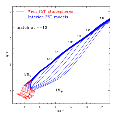
As no available theory is self consistent, the dominant attitude in stellar studies –unless there are particular requirements– is to use the convective model as a ‘black box’ simply to infer the stellar properties in the region in which convection becomes adiabatic. In general, in fact, the main important property which a convection model is required to provide is the stellar radius: whatever is in the ‘black box’ of convection, we first of all wish to know the radius (or the , or, equivalently, the entropy jump between the adiabatic interior and the surface). The solar radius in particular is generally adjusted in the models by varying the convective efficiency. In the MLT this can be done by varying the ‘mixing length’ parameter, that is the ratio of mixing length to pressure scale height . Recently it has been stressed the importance of surpassing the Eddington approximation, or the gray atmosphere approximations to correctly describe the optical atmosphere. For many stellar situations, a non gray model atmosphere —which also must reproduce the observed spectral features— includes as necessary ingredient a treatment of convection, which, in the MLT, will be characterized by a given down to the optical depth at which the atmosphere will be matched to the interior computation. In the interior, convection will be characterized by a given . Thus, actually, a ‘modern’ MLT structure will have three parameters: , and . Figure 9 illustrates this classic problem by using our recent models ([\astronciteMontalbán et al.2003]) which adopt as boundary conditions the NextGen atmospheric grid ([\astronciteAllard et al.1997], hereinafter referred to as AH97), computed by assuming MLT convection with , down to optical depth .
Adopting for the interior computations, we obtain a set of tracks, among which the solar track passes through the solar location at the solar age. The solar mass track with , on the contrary, is K cooler at the solar luminosity. This well known fact remembers how large is the variation in allowed by changing the MLT parameter. The meaning of this solar radius adjustment is simply the following: when using the MLT, the entropy jump, necessary to fit the solar , between the adiabatic layers and the surface corresponds to what is obtained with the MLT and up to , and with MLT and up to the surface. Of course, the model can not tell us anything about the temperature gradient layer by layer within the envelope. If we only wish to use convection as a ‘black box’, we just take the model for the Sun111and generally we forget, or at least do not even mention, that is actually for most of the overadiabatic region, which is contained in the model atmosphere grid.. Of course, our assumption will only be valid for the Sun itself.
An interesting broadening of of this point of view to a wider part of the HR diagram has been given by [*]ludwig99, who performed detailed 2D numerical RHD calculations of time-dependent compressible convection, in the range 4300 7100K, 2.544.74 (cgs) for solar composition. They used these models to ‘calibrate’ the effective for these envelopes, that is the value of which provides the same specific entropy jump (using a gray atmosphere, therefore this approximation defines a unique average parameter) than their 2D models. They found values from 1.3Hp for F dwarfs up to 1.8Hp for K giants. This calibration of , again, does not tell us anything about the temperature gradient layer by layer.
The approach of keeping convection as an entirely black box is very useful, but it has –obviously– many limitations. In particular, if we wish to study the excitation of oscillation instabilities in stars we must know the full stratification of physical quantities in the star, up to the atmosphere.
4 Convection modelling in full stellar models
We have to recognize that no general purpose convection model is presently available, which can be meaningfully applied to any stellar structure in order to know the layer by layer stratification of physical quantities. Nevertheless, recently there have been several attempts to produce entire stellar models, which satisfy some observational constraints on the atmospheric and envelope convection, and in which the atmospheric and the envelope convection are matched ‘smoothly’ each other. A smooth match is at least technically necessary for stellar stability studies, to avoid discontinuities in the physical quantities. A prototype of these models has been discussed by [*]schlattl1997 for the Sun. They built up a non gray 1D model atmosphere with down to , and matched it to a subatmosphere and MLT interior, guided by the results of 2D hydro models. To do this, they had to vary the parameter in the interior computation, with the aim to provide the solar radius and obtain a temperature stratification similar to that of the 2D models. The aim of this study was to explore the influence of the physical inputs on the solar p–modes.
Of course, for the Sun we have an enormous number of constraints —from the p–modes themselves, and from the precise knowledge of the solar radius— which help to build up a fully parametric model. But what should we do to extend the analysis to other stars? What kind of model atmosphere can we use, and how do we produce a ‘meaningful’ match of the atmospheric and interior computation? There are not yet many model atmosphere grids available, and many of them have been computed for “atmospheric purposes” only, that is to produce an adequate modelling of the region from which the stellar spectum emerges, so they are not entirely apt to be used as boundary conditions for full stellar models. For instance, the quoted AH97 models, computed with the PHOENIX code, adopt MLT convection with and a total of 50 layers down to . [*]heiter2002 have adopted a new version of Kurucz’s ([\astronciteKurucz1993]) model atmospheres (the Vienna–ATLAS9 code), in which the convection model is either the MLT with or the FST (both in the [\astronciteCanuto & Mazzitelli1991] and in the [\astronciteCanuto et al.1996] versions), and they have increased the number of layers in the latter models to 288. We have recently used all these grids of model atmospheres to explore the meaning of the match between atmosphere and interior, and what happens when one extends to other models (pre main sequence, and giants) the approximations adopted for the solar model. The extensive results of this study are presented elsewhere ([\astronciteMontalbán et al.2003]). Here we show, in Figure 1, that the different solar models which can be built up, all satisfying the constraint of the solar fit, can have very different subatmospheric structures, depending on the choice of the convection efficiency in the different layers.
In Figure 1 we also see that the model adopting the FST convection both in the atmosphere and in the interior does not show discontinuities in the T vs. P stratification. The structure smoothly passes from a very inefficient convection in the atmosphere, similar to that of the MLT models with , to such an efficient convection inside, that the precise solar fit is easily obtained (see e.g. [\astronciteCanuto & Mazzitelli1991])222Remember that, whatever the choice of the free parameters in the FST convection, it is not possible to obtain a 1location, at L⊙, with much smaller or larger than the solar , contrary to the MLT models..
Computing “full FST” structures, then, has as a first a “formal” advantage, as it helps to avoid the problem of discontinuities in the physical quantities for instability studies. In addition, there are other, more physical, reasons to use this model as probe: a series of works on 1) determination from Hα and Hβ lines (e.g. [\astronciteFuhrmann et al.1993]; [\astroncitevan’t Veer-Menneret et al.1996]); 2): theoretical predictions of Hα and Hβ from 1D models ([\astronciteGardiner et al.1999]) and from 2D models ([\astronciteSteffen & Ludwig1999]); 3): theoretical predictions of and Strömgren indices ([\astronciteSmalley & Kupka1997]) and abundance determinations ([\astronciteHeiter et al.1998]) indicate that, even if a 1D, homogeneous model can not explain all the spectroscopic and photometric observations, model atmospheres which predict temperature gradients closer to the radiative gradient are in better overall agreement with the observations. These arguments favors those models in which convection in the atmosphere is less efficient than predicted by models having ), and led [*]heiter2002 to adopt either the FST model or the MLT models to compute their atmospheric grids. These were also further motivations to produce “full FST” stellar models by use of their atmospheric grids.
We may ask whether the “full FST” models have shown features interesting enough to render it useful to explore the application of the FST convection in different parts of the HR diagram. We give here one positive example (the interpretation of the Böhm–Vitense gap at B–V) and one “negative” example, namely the impossibility of explaining the patterns of Lithium depletion in the Sun and in open clusters with the FST model. This latter result, however, may be telling us something else on the behaviour of convection in young convective stars.
5 The Böhm Vitense gap at B–V
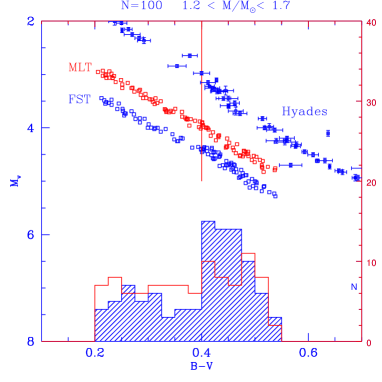
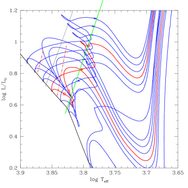
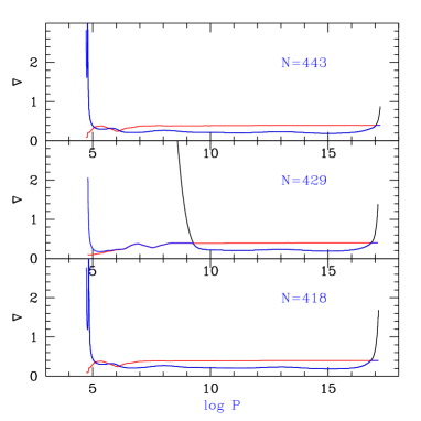
One of the most interesting results in our recent exploration of “full” FST models regards the main sequence: the FST convection, due to its very low efficiency close to the stellar surface, and high efficiency in the inner subatmospheres, yields a very sharp transition between structures which are convective only in the surface layers, and structures which show a well developped convection also in the interior ([\astronciteD’Antona et al.2002]) . This is shown in Figure 2 by comparing the stratification of models of different mass in the P–T plane: models down to 1.42 are mostly radiative (or convection is so inefficient that the convective gradient sticks very close to the radiative one), while suddenly, at 1.41, an extended adiabatic convection region appears for a larger part of the envelope. The fast increase in the convective mass fraction () as a function of the main sequence color B–V is shown in Figure 3. This characteristic of the models is reflected in their mass– relation, which becomes suddenly steeper around K, and is also apparent in the HR diagram as a sudden change of slope (Figure 3). Using numerical simulations we have shown that this feature produces a stellar depletion which is consistent with the gap seen in the Hyades at 0.33 B–V 0.38, one of the so called “Böhm Vitense gaps” after [*]bvcanterna1974 and [*]bv1982, found by [*]rachford-canterna2000 in 6 our of 9 open clusters which have been investigated. The standard MLT models do not show this behavior (see Figure 4).
The very sharp variation of the stellar structures in the HR diagram (or in the gravity plane) is shown as a transition line in the HR diagram of Figure 5. Models on the right of this line have extended convective regions, and models on the left have very small convective regions, independently from their evolutionary phase (pre, on or post the main sequence). This can be seen in Figure 6. The transition line is compared in Figure 5 with the location of the Scuti and Doradus instability strips. We may speculate that our transition line separates HR diagram regions which harbor different modalities of stellar oscillation patterns, as the excitation or driving mechanisms can be very different for stars having so different convective structure. In particular, it could represent the dividing line between coherent pulsations and solar-type oscillations. In this case, we should have expected that also the stars between the red edge of the Doradus instability strip and the transition line are pulsating. Notice that the location of the red edge of the Doradus strip is based on observations from the ground and might still be uncertain in the theoretical HR diagram. On the other hand, many other structural parameters may have a role in defining these instability strips, and at least two of these —elements diffusion and rotation— should be considered. A further note of caution on the naivety of this proposal comes also from the complex behavior of the chromospheric and transition layer indicators for the MS stars on the right of the transition line ([\astronciteBöhm-Vitense et al. 2002]).
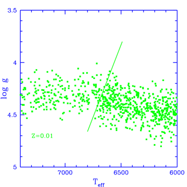
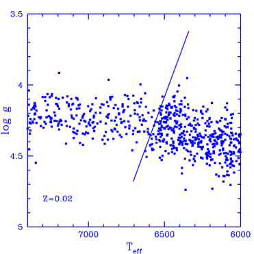
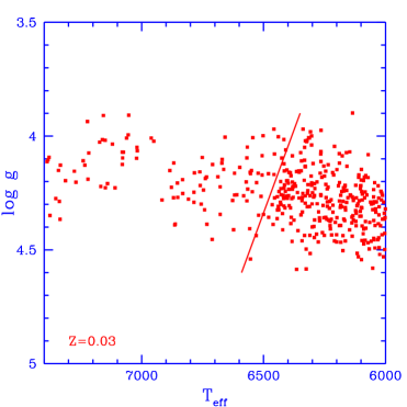
Will the Böhm Vitense gap appear also in the field stars? Here the problem will be much more complicated by the blurring due to the fact that we have a mixture of ages and metallicities! Figure 7 shows simulations for three stellar populations with different metallicities (Z=0.01, 0.02 and 0.03), covering ages from 107 to 109yr, and distributed according to a Salpeter mass function. The diagonal lines separate the location of the models having deep envelope convection (at cooler ) from those, hotter, having very thin atmospheric convection. A gap is apparent on the left of each line, which shift to cooler with increasing metallicity, so that it will not be easy to locate a gap in a sample of stars not homogeneous in metallicity.
6 The ‘historical’ problem of Lithium
In the years 1965-1990, we called ‘problem of lithium in the Sun’ the inhability of the solar mass evolutionary tracks to burn a substantial fraction of their initial lithium during the Pre Main Sequence (PMS). This result was generally taken as a good proof that additional mechanisms for depletion were required, acting during the long solar MS lifetime, to reduce by a factor 140 the initial solar system abundance ( N(Li)=3.31 ([\astronciteAnders & Grevesse1989]). This interpretation still today is taken as most plausible one, confirmed by the scarce lithium depletion, at the solar mass, in young open clusters (see e.g. [\astronciteChaboyer1998]). In fact the lithium vs. relation for the MS stars of young open clusters indicates a lithium depletion by at most a factor two for the solar mass in young clusters, while it is compatible with the solar depletion in some stars of the cluster M67, close to the solar age. For recent reviews see e.g. [*]jeffries2000 and [*]pasquini2000.
However, a different problem emerges from the most recent computation of solar models: they deplete too much lithium during the PMS evolution ([\astronciteD’Antona & Mazzitelli1994], [\astronciteD’Antona & Mazzitelli1997], [\astronciteSchlattl & Weiss1999], [\astroncitePiau & Turck-Chièze2000]) and are incompatible with the young open clusters observations. This problem is most severe in models using very efficient convection models, in fact it is more relevant for the D’Antona and Mazzitelli (1994 and 1997) models adopting the FST convection. MLT models of the most recent generation, adopting updated equations of state and opacities also deplete too much lithium. [*]dm2003 have recently reappreciated that the problem is severe in tracks whose convection is adjusted to provide the solar radius at the solar age! If one does not require the solar fit, it is easy to decrease the convection efficiency and to obtain a negligible PMS lithium depletion.
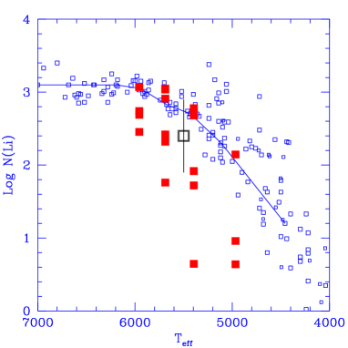
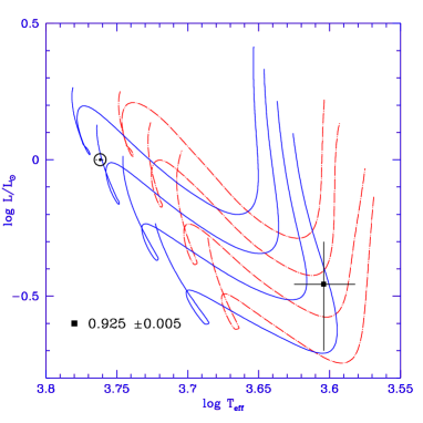
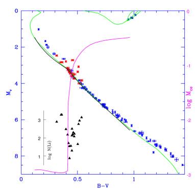
In Fig. 8 we compare the lithium depletion predicted by many of our models, computed using AH97 atmospheres () as boundary conditions, with the Pleiades data by [*]soderblom1993 and [*]garcialopez1994. Only the upper squares, corresponding to the models employing , which do not fit the Sun, are compatible with the data. The HR diagram of the models is shown in Figure 9. The tracks are on the right, much cooler than what is needed to allow the solar fit! In addition, Figure 9 opens up the complex problem of the location in the HR diagram of PMS tracks (for a review see, e.g. [\astronciteD’Antona et al. 2000], while our full recent computation for this phase can be found in [\astronciteMontalbán et al.2003]). When we compare the location of PMS theoretical tracks with the observed few data of PMS stars for which an independent determination of mass is available333these stars either belong to binaries (e.g. [\astronciteCovino et al.2001], [\astronciteSteffen et al.2001)], or one can measure the stellar mass from the dynamical properties of their protoplanetary disks ([\astronciteSimon et al.2000])., the tracks most consistent with the observations are again those with cooler atmospheres (higher mass for a given spectral type) and thus those which, generally, provide a radius larger than R⊙ for the solar model. In fact, Figure 9 shows that the tracks are well compatible with the location of the secondary component of the eclipsing spectroscopic binary RXJ 0529.4+0041, one of the best determined PMS masses ([\astronciteCovino et al.2001]. It is then clear that 1) the HR diagram location of the tracks during the PMS evolution, and 2) PMS lithium depletion, are two problems correlated each other, as it could have been expected, because, the smaller the of the Hayashi track, the smaller is the temperature at the base of the convective envelope during the possible phase of lithium burning. Both the HR diagram location and the lithium depletion seem to be compatible only with models in which PMS convection is much less efficient than MS convection. Is this simply another proof that we are not able to model convection, or that there are unsolved problems with the opacities? Or does it mean that there is some other parameter playing a role in the PMS –and not on the MS? It is probably too early to derive strong conclusions, but we have suggested that PMS convection is inhibited by the thermal role of a dynamo built magnetic field ([\astronciteVentura et al.1998b], [\astronciteD’Antona et al. 2000]).
7 Non-local convection in the Sun
Always in the framework of stellar evolution for asteroseismology, we performed one more consistency test, of a completely different nature. In this case, our attention is not at the surface, but at the bottom of the solar convective zone (CZ). In fact, a constraint to the thickness of the overshooting layer in this region has been set by helioseismology (e.g. [\astronciteBasu & Antia1997]), and it can not be larger than 0.05. We constructed a detailed FST solar model matching the correct thickness of the CZ (the surface boundary condictions are in this case of negligible importance) and applied the treatment suggested by [\astronciteCanuto & Dubovikov1998] (CD98) to a thin region centered around the formal Schwarzschild boundary of convection, to gain insight on what happens when a fully non-local turbulence theory is applied to a stellar structure.
More in detail, we have computed from the local model the starting distribution for the quantities: (turbulent kinetic energy in the radial direction), (mean quadratic temperature variance), (convective flux), (mean quadratic velocity variance) and (dissipation rate), according to (42a-c), (43a-c) and (44a-d) in CD98. Then, temporal relaxation to the five above quantities has been allowed, according to the equations (19a-d) and (35a-b), until stationary conditions were reached. For each relaxation step, the gradient :
| (1) |
has been updated according to:
| (2) |
where is the thermometric conductivity, . Further, is the kinetic energy flow and is the turbulent viscosity, .
Eq. (18c) from CD98, relative to the temperature, was not included in the final network since, being superadiabaticity at the bottom of the solar CZ negligible, temperature itself turned out to be nearly stationary already at the beginning of the relaxation.
As for the diffusive terms , the most simple down-gradient approximation has been chosen, namely, for each generic turbulent quantity :
| (3) |
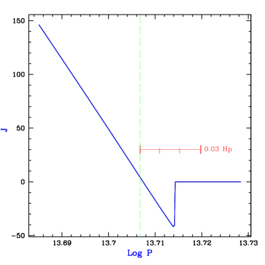
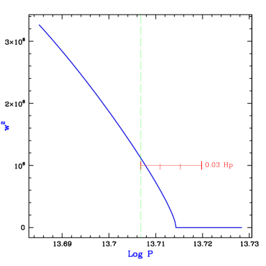
This is (perhaps) far from the best one can do but, noticeably, no built-in scale length is present, contrarily to the only other non-local treatment ([\astronciteXiong1985]) with which extensive stellar models have been computed. In fact, in Xiong case, an explicit, arbitrary scale length was included, and the results almost linearly depended on the value of the scale length. After s, all the six quantities (including ) reached a final, stationary distribution, clearly showing a thin overshooting region. Figure 10 shows the behavior of the turbulent flux ; Figure 11 presents the mean quadratic velocity variance . Overshooting is present indeed, but its amplitude does not overcome 0.02, consistently with the solar observational constraints.444The very sharp decline of the flux is an important constraint for the ‘local’ parametrization of overshooting. In particular, it is different from the approximation of exponential decay adopted, e.g., by [\astronciteVentura et al.1998a] and [\astronciteHerwig et al.1997]. These results apply only to overshooting below the CZ, we can not extend them to what happens above the convective cores. The same relaxations have been performed for the CZ of the solar mass track at various evolutionary phases, from the first appearence of a radiative nucleus in PMS, up to early red giant. The overall features turn out to be similar in all cases. It is found that the overshooting region is absolutely negligible () in PMS during the lithium burning phase. This at least ensures us that inclusion of proper overshooting in PMS evolutionary models will not worsen the problems with the exceedingly large solar lithium depletion shown by todays standard models. The thickness of overshooting, then, steadily increases during the evolution, reaching at , where the computations have been stopped. In all case, the decay of is very sharp, putting an end to overshooting.
The only conclusion we can presently draw from these first non-local results is that probably the chosen approximation for the diffusive terms is perhaps not too bad, at least as long as the thickness of overshooting is concerned, since they are consistent with the observational solar constraints, and do not worsen the lithium problem.
Acknowledgements.
This work has been partially supported by the MIUR through the COFIN 2002-2003 project “Asteroseismology’.References
- [\astronciteAllard et al.1997] Allard F., Allard, F., Hauschildt, P. H., Alexander, D. R., & Starrfield, S. 1997, Annu. Rev. A.&A., 35, 137
- [\astronciteAnders & Grevesse1989] Anders E., Grevesse N., 1989, Geochim. Cosmochim. Acta 53, 197
- [\astronciteBasu & Antia1997] Basu, S. & Antia, H. M. 1997, MNRAS, 287, 189
- [\astronciteBoesgaard & Tripicco 1986] Boesgaard, A.M., & Tripicco, M.J. 1986, ApJ, 302, L49
- [\astronciteBöhm-Vitense1958] Böhm-Vitense, E. 1958, Z. Astrophys., 46, 108
- [\astronciteBöhm-Vitense1970] Böhm-Vitense, E. 1970, A&A, 8, 283
- [\astronciteBöhm-Vitense & Canterna1974] Böhm-Vitense, E. & Canterna, R. 1974, ApJ, 194, 629
- [\astronciteBöhm-Vitense1982] Böhm-Vitense, E. 1982, ApJ, 255, 191
- [\astronciteBöhm-Vitense et al. 2002] Böhm-Vitense, E., Robinson, R., Carpenter, K., & Mena-Werth, J. 2002, ApJ, 569, 941
- [\astronciteCanuto & Mazzitelli1991] Canuto, V. M. & Mazzitelli, I. 1991, ApJ, 370, 295
- [\astronciteCanuto & Dubovikov1998] Canuto, V. M. & Dubovikov, M. 1998, ApJ, 493, 834
- [\astronciteCanuto et al.1996] Canuto, V. M., Goldman, I., & Mazzitelli, I. 1996, ApJ, 473, 550
- [\astronciteChaboyer1998] Chaboyer B., 1998, In: Deubner F.-L, Christensen-Dalsgaard J., Kurtz D. (eds.) ‘New eyes to see inside the sun and stars’. IAU Symp. 185. p. 25
- [\astronciteCovino et al.2001] Covino E., Melo C., Alcalá J.M., Torres G., Fernández M., Frasca A., and Paladino R. 2001, A&A 375, 130
- [\astronciteD’Antona2000] D’Antona, F. 2000, Star formation from the small to the large scale. ESLAB symposium (33 : 1999 : Noordwijk, The Netherlands). Edited by F. Favata, A. Kaas, and A. Wilson. Proceedings of the 33rd ESLAB symposium on star formation from the small to the large scale, ESTEC, Noordwijk, The Netherlands, 2-5 November 1999 Noordwijk, The Netherlands: European Space Agency (ESA), 2000. ESA SP 445., p.161, 445, 161
- [\astronciteD’Antona & Mazzitelli1994] D’Antona F., Mazzitelli I., 1994, ApJS 90, 467 (DM94)
- [\astronciteD’Antona & Mazzitelli1997] D’Antona F., Mazzitelli I., 1997, in “Cool stars in Clusters and Associations”, eds. G. Micela and R. Pallavicini, Mem. S.A.It. 68, 807
- [\astronciteD’Antona & Montalbán2003] D’Antona F., & Montalbán J. 2003, A&A, in press
- [\astronciteD’Antona et al. 2000] D’Antona, F., Ventura, P., & Mazzitelli, I. 2000, ApJL, 543, L77
- [\astronciteD’Antona et al.2002] D’Antona F., Montalbán J., Kupka F., Heiter U., 2002, ApJ 564, L93
- [\astroncitede Bruijne et al.2000] de Bruijne, J. H. J., Hoogerwerf, R., & de Zeeuw, P. T. 2000, ApjL, 544, L65
- [\astroncitede Bruijne et al.2001] de Bruijne, J. H. J., Hoogerwerf, R., & de Zeeuw, P. T. 2001, A&A, 367, 111
- [\astronciteFuhrmann et al.1993] Fuhrmann, K., Axer, M., & Gehren, T. 1993, A&A, 271, 451
- [\astronciteGarcia Lopez et al.1994] Garcia Lopez, R. J., Rebolo, R., & Martin, E. L. 1994, A&A, 282, 518
- [\astronciteGardiner et al.1999] Gardiner, R. B., Kupka, F., & Smalley, B. 1999, A&A, 347, 876
- [\astronciteHeiter et al.1998] Heiter, U., Kupka, F., Paunzen, E., Weiss, W. W., & Gelbmann, M. 1998, A&A, 335, 1009
- [\astronciteHeiter et al.2002] Heiter, U., Kupka, F., van’t Veer-Menneret, C., Barban, C., Weiss, W.W., Goupil, M.J., Schmidt, W.W., Garrido, R. 2002, A&A, 392, 619
- [\astronciteHerwig et al.1997] Herwig, F., Bloecker, T., Schoenberner, D., & El Eid, M. 1997, A&A, 324, L81
- [\astronciteJeffries2000] Jeffries, R. D. 2000, ASP Conf. Ser. 198: Stellar Clusters and Associations: Convection, Rotation, and Dynamos, 24
- [\astronciteKurucz1993] Kurucz, R.L. (1993), CDROM13: ATLAS9, SAO, Harvard, Cambridge
- [Kupka (1999)] Kupka, F. 1999, ApjL, 526, L45
- [\astronciteKupka & Montgomery2002] Kupka F., Montgomery M.H., 2002, MNRAS, 330, L6
- [\astronciteLudwig et al.1999] Ludwig, H.–G., Freytag, B., & Steffen, M. 1999, A&A, 346, 111
- [\astronciteMazzitelli & D’Antona1993] Mazzitelli, I., & D’Antona, F. 1993, in Inside the stars; Proceedings of the 137th IAU Colloquium, Univ. of Vienna, Austria, Apr. 13-18, 1992, p. 457
- [\astronciteMontalbán et al.2003] Montalbán, J., D’Antona F., Kupka F., Heiter, U., 2003, A&A submitted
- [\astroncitePamyatnykh2000] Pamyatnykh, A.A. 2000, in “Delta Scuti and Related Stars”, eds. M. Breger and M.H. Montgomery, ASP Conf. Series 210, 215
- [\astroncitePasquini2000] Pasquini, L. 2000, IAU Symposium, 198, 269
- [\astroncitePiau & Turck-Chièze2000] Piau, L. & Turck-Chièze, S. 2002, , 566, 419
- [\astronciteRachford & Canterna2000] Rachford, B. L. & Canterna, R. 2000, AJ, 119, 1296
- [\astronciteSchlattl et al.1997] Schlattl, H., Weiss, A., & Ludwig, H.–G. 1996, A&A, 322, 646
- [\astronciteSchlattl & Weiss1999] Schlattl, H. & Weiss, A. 1999, A&A, 347, 272
- [\astronciteSimon et al.2000] Simon, M., Dutrey, A., & Guilloteau, S. 2000, ApJ, 545, 1034
- [\astronciteSmalley & Kupka1997] Smalley, B. & Kupka, F. 1997, A&A, 328, 349
- [\astronciteSoderblom et al.1993] Soderblom, D. R., Jones, B. F., Balachandran, S., Stauffer, J. R., Duncan, D. K., Fedele, S. B., & Hudon, J. D. 1993, AJ, 106, 1059
- [\astronciteSteffen & Ludwig1999] Steffen, M. & Ludwig, H.-G. 1999, ASP Conf. Ser. 173: Stellar Structure: Theory and Test of Connective Energy Transport, 217
- [\astronciteSteffen et al.2001)] Steffen, A. T. et al. 2001, AJ, 122, 997
- [\astroncitevan’t Veer-Menneret et al.1996] van’t Veer-Menneret C., Megessier C., 1996, A&A 309, 879
- [\astronciteVentura et al.1998a] Ventura, P., Zeppieri, A., Mazzitelli, I., & D’Antona, F. 1998a, A&A, 334, 953
- [\astronciteVentura et al.1998b] Ventura, P., Zeppieri, A., Mazzitelli, I., & D’Antona, F. 1998b, A&A, 331, 1011
- [\astronciteVentura et al.2001] Ventura, P., D’Antona, F., Mazzitelli, I., & Gratton, R. 2001, ApjJL, 550, L65
- [\astronciteXiong1985] Xiong, D. R. 1985, A&A, 150, 133
- [\astronciteZerbi2001] Zerbi, F.M. 2000, in “Delta Scuti and Related Stars”, eds. M. Breger and M.H. Montgomery, ASP Conf. Series 210, 332