The current status of observational cosmology

Abstract

Observational cosmology has indeed made very rapid progress in recent years. The ability to quantify the universe has largely improved due to observational constraints coming from structure formation. The transition to precision cosmology has been spearheaded by measurements of the anisotropy in the cosmic microwave background (CMB) over the past decade. Observations of the large scale structure in the distribution of galaxies, high red-shift supernova, have provided the required complementary information. We review the current status of cosmological parameter estimates from joint analysis of CMB anisotropy and large scale structure (LSS) data. We also sound a note of caution on overstating the successes achieved thus far.

1. Introduction

Recent developments in cosmology have been largely driven by huge improvement in quality, quantity and the scope of cosmological observations. The measurement of temperature anisotropy in the cosmic microwave background (CMB) has been arguably the most influential of these recent observational success stories. A glorious decade of CMB anisotropy measurements has been topped off by the data from the Wilkinson Microwave Anisotropy Probe (WMAP) of NASA. Observational success has set off an intense interplay between theory and observations. While the observations have constrained theoretical scenarios and models more precisely, some of these observations have thrown up new challenges to theoretical understanding and others that have brought issues from the realm of theoretical speculation to observational verification. The results the WMAP mission on CMB anisotropy  [?] and the power spectrum of density perturbations from the 2-degree field (2dF) survey of galaxies  [?] and the Sloan Digital Sky Survey (SDSS) of galaxies [?], have allowed very precise estimation of cosmological parameters  [?,?,?].

These results have been widely heralded as the dawn of precision cosmology. To a casual science observer, the unprecedented precision in determining the parameters of the standard cosmological model often conveys the false impression that we actually know and understand the components that make up the universe, we know its primeval history (including the theoretical scenarios of baryogenesis and inflation) and evolution including growth of large scale structures. The reality is that our understanding of some of the components is limited to very rudimentary characterization, e.g., in terms of their cosmic energy density, velocity dispersion, equation of state etc. Besides the obvious need for direct detection, we are not quite in a position even to rule out equally viable non-standard alternatives.

The cosmological model can be broadly split into two distinct aspects: the nature and dynamics of the homogeneous background and, the origin and evolution of perturbations leading to the large scale structure in the distribution of matter in the universe. It is certainly fair to say that the present edifice of the standard cosmological models is robust. A set of foundation and pillars of cosmology have emerged and are each supported by a number of distinct observations:

• Homogeneous, isotropic cosmology, expanding from a hot initial phase due to gravitational dynamics of the Friedman equations derived from the laws of general relativity.

• The basic constituents of the universe are baryons, photons, neutrinos, dark matter and dark energy (cosmological constant/vacuum energy).

• The homogeneous spatial sections of space-time are nearly geometrically flat (Euclidean).

• Generation of primordial perturbations in an inflationary epoch. The primordial density perturbations are adiabatic with a nearly scale invariant power spectrum. Imprint of these perturbations on CMB anisotropy indicates correlation on a scale larger than the causal horizon. Polarization of the CMB anisotropy provides even stronger support for adiabatic initial conditions and the apparently ‘acausal’ correlation in the primordial perturbations.

• Evolution of density perturbations under gravitational instability has produced the large scale structure in the distribution of matter.

The past few years have seen the emergence of a ‘concordant’ cosmological model that is consistent with observational constraints from the background evolution of the universe as well as with those from the formation of large scale structures.

The emergent concordance cosmological model does face challenges from future observations. For example, the detection of the inflationary gravity wave in B-mode of CMB polarization would be needed to clinch the case for inflation. The current observations have also revealed potential cracks in the cosmological model which need to be resolved through improved theoretical computations and improved future observations. An example is the inability to recover the profile and number density of cusps in the halos with the standard (collision-less) cold dark matter.

2. Observations of the cosmological model

The evolution of the universe is an initial value problem in general relativity that governs Einstein’s theory of gravitation. Under the assumptions of large scale homogeneity and isotropy of space (spatial sections in a foliation of space-time), the dynamics of the spatial sections reduces to the time evolution of the scale factor $a(t)$ of the spatial section. Further, the components (species) of matter are assumed to be non-interacting (on cosmological scales), ideal, hydrodynamic fluids, specified by their energy/mass density $\rho$ and the pressure $p$ (equivalently, by the equation of state $w$ where $p=w\rho$). The density of any component $i$ then evolves in the expanding universe as $\rho_{i}=\rho_{\rm 0i}a^{-3(1+w_{i})}$. The simple Friedman equation

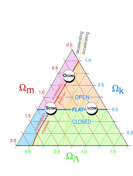
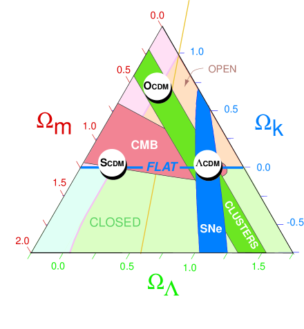
Figure  1.: The Cosmic Triangle represents the three key cosmological parameters – $\Omega_{m}$, $\Omega_{\Lambda}$, and $\Omega_{k}$ – where each point in the triangle satisfies the sum rule $\Omega_{m}+\Omega_{\Lambda}+\Omega_{k}=1$. The blue horizontal line (marked Flat) corresponds to a flat universe ($\Omega_{m}+\Omega_{\Lambda}=1$), separating an open universe from a closed one. The red line, nearly along the $\Lambda=0$ line, separates a universe that will expand forever (approximately $\Omega_{\Lambda}>0$) from one that will eventually recollapse (approximately $\Omega_{\Lambda}<0$). And the yellow, nearly vertical line separates a universe with an expansion rate that is currently decelerating from one that is accelerating. The location of three key models are highlighted: (flat) standard cold-dark-matter (Scdm) ; flat ($\Lambda$cdm); and Open CDM (Ocdm). The right panel schematically shows the complementarity of constraints ($\sim 1\sigma$) from LSS, High-z SN Ia, and CMB anisotropy are shown by the three color bands.The three independent bands intersect at the emergent concordance model – flat model with $\Omega_{m}\sim 0.3$ and $\Omega_{\Lambda}=0.7$.

$$H^{2}(t)\equiv\left(\frac{\dot{a}}{a}\right)^{2}=\frac{8\pi G}{3}~{}\left[\rho_{\rm 0m}a^{-3}+\rho_{\rm 0r}a^{-4}+\rho_{\Lambda}+\rho_{\rm 0K}a^{-2}\right]$$ (1)

that arises from the Einstein equations relates the Hubble parameter $H(t)$ that measures the expansion rate of the universe to the present matter density in the universe. Dividing by $H^{2}$ on both sides leads to a simple sum rule

$$\Omega_{\rm m}+\Omega_{\rm r}+\Omega_{\Lambda}+\Omega_{\rm K}=1\,,$$ (2)

where we use the conventional dimensionless density parameter $\Omega_{i}=\rho_{i}/\rho_{\rm c}$ in terms of the critical density $\rho_{\rm c}=3H^{2}/8\pi G$. The key components of the universe are relativistic matter (eg., radiation) $\Omega_{\rm r}$, pressure-less gravitating matter $\Omega_{\rm m}$, cosmological vacuum (dark) energy, $\Omega_{\Lambda}$. The departure of the total matter density parameter from unity contributes to the curvature of the space and can, hence, be represented by an effective curvature energy density, $\Omega_{K}$ that determines the effect of curvature on the expansion of the universe. The relativistic matter density is almost entirely dominated by the cosmic microwave background (CMB) and the relic background of massless neutrinos. The isentropic expansion dictated by the Friedman equations implies that although $\Omega_{\rm r}$ makes a negligible contribution at present given by the temperature of the CMB, at an early epoch the universe was dominated by relativistic matter density. The pressure-less matter density $\Omega_{\rm m}=\Omega_{\rm B}+\Omega_{\rm cdm}+\Omega_{\nu}$ minimally consists of three distinct components, the baryonic matter, cold dark matter, and a minor contribution from massive neutrino species. The dark energy density could well be an exotic, ‘non-clustering’ matter with a variable equation of state, $w(z)<-1/3$. In this article, we limit our attention to the simplest case of a cosmological constant with a constant equation of state, $w=-1$.

The present state of the universe in terms the three dominant components can neatly be summarized on the ‘cosmic triangle’ shown in figure 1  [?]. The three axes address fundamental issues regarding the background cosmology – does space have positive, negative or zero curvature, whether the expansion is accelerating or decelerating, and, the issue of the non-relativistic matter budgets? The current cosmological observations have definitively determined the present universe to be located in the $\Lambda$-cdm region and far removed from the past favorites, the canonical standard cold dark matter (Scdm) and open cold dark matter (Ocdm) models with high statistical significance.

Some of the cosmological parameters are well-estimated by observations that probe the background evolution of the universe. The latest constraint on the baryon density, $\Omega_{\rm B}h^{2}=0.022\pm 0.002$ obtained by matching the predicted abundances of light elements from Big Bang nucleosynthesis with observations  [?] is consistent with that recently obtained from considerations of structure formation  [?,?,?].

The energy density of the cosmological constant (or, more broadly quintessence) can be inferred from the measurement of luminosity distance as a function of red-shift using high red-shift supernova SN Ia as standard candles. The recent results using supernova indicate that $\Omega_{\Lambda}-1.4\Omega_{\rm m}=0.35\pm 0.14$  [?]. For a flat universe (indicated by CMB+LSS data), $\Omega_{\rm m}=0.29\pm 0.05$ and the equation of state $w=-1.02\pm 0.2$ is consistent with a cosmological constant. Further, the analysis including new SN Ia observations from HST concludes that allowing for a variable equation of state, $w(z)$, there is no evidence for any rapid variation  [?]. As mentioned below, this is consistent with the constraints from the CMB anisotropy and large scale structure observations and combined constraints are remarkably tight around the cosmological constant.

Measuring the expansion rate of the universe, $H_{0}=100h$ km s^-1/Mpc was a key project of the Hubble space telescope mission. The current estimates are $h=0.72\pm 0.07$  [?]. The high-$z$ SN Ia results also constrain the combination $H_{0}t_{0}=0.96\pm 0.04$ implying an age $t_{0}=13.6\pm 1.5\,\,\,\rm Gyr$ when combined with the HST determination of $H_{0}$. The expansion rate and age estimates are again consistent with, and considerably improved by including structure formation consideration as discussed below.

3. Structure formation in the universe

The ‘standard’ model of cosmology must not only explain the dynamics of homogeneous background universe, but also (eventually) satisfactorily describe the perturbed universe – the generation, evolution and finally, the formation of large scale structures in the universe. It is fair to say that much of the recent progress in cosmology has come from the interplay between refinements of the theories of structure formation and the improvement of the corresponding observations.

The CMB anisotropies are the imprints of the perturbed universe in the radiation. On the large angular scales, the CMB anisotropy directly probes the primordial power spectrum on scales enormously larger than the ‘causal horizon’ at the epoch of last scattering at a red-shift, $z\sim 1100$. On smaller angular scales, the CMB temperature fluctuations probe the physics of the coupled baryon–photon fluid through the imprint of the acoustic oscillations in the ionized plasma sourced by the same primordial fluctuations. The physics of CMB anisotropy is well-understood, the predictions (of the linear primary anisotropy) and their connection to observables are unambiguous  [?,?]. The remarkable success of the measurements of the CMB angular power spectrum $C_{l}$ over the past decade leading up to the recent WMAP results is covered elsewhere in these proceedings (see p. — of Pramana – J. Phys. 64(4), (2004)).

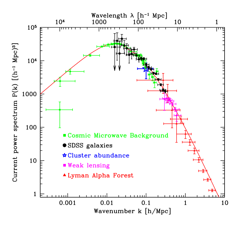
Figure  2.: Figure taken from [2] shows that the current estimate of the linear power spectrum, $P(k)$ of ‘density’ perturbations comes from a number of distinct cosmological observations of spectrum of cosmological perturbations . At low wave numbers $k$, the $P(k)$ is inferred from the angular power spectrum of the CMB anisotropy. At the high $k$ end, the $P(k)$ is measured from the Ly-$\alpha$ forest. The intermediate regime, is probed by distribution of galaxies in the large scale surveys (here,SDSS). The measurements from these different measurements line up along the theoretical predictions of the currently favored cosmology.

In its totality, quantifying and understanding the observed large scale structures in the universe involves complex, non-linear aspects of gravitational instability and baryon ‘gastrophysics’. However, in estimating cosmological parameters the observational constraints from structure formation on scales larger than $\sim$10$h^{-1}\ {\rm Mpc}$ are dominant. At present, the constraints come from the measured linear power spectrum of density perturbations $P(k)$. As shown is figure 2, for small values of the wave number, $P(k)$ are probed by the CMB anisotropy spectrum. On the intermediate wave numbers, $P(k)$ is measured by the ongoing large surveys of galaxies such as the SDSS and 2 degree field  [?,?]. The power spectrum at the largest wave numbers considered here is measured from the one-dimensional distribution of absorption features along the line of sight to quasars  [?].

There is a well-understood (if not rigorously defined) notion of a ‘standard’ model of cosmology that includes the formation of large scale structure. Table 1 is an illustrative list of parameters that characterize a cosmology in terms of background evolution as well as structure formation  [?]. Variations on the choice, as well as, combinations of the parameters are possible and have been used. More importantly, these constitute a kind of ‘minimal’ accepted set. We often need to extend the set of parameters. In particular, it is important to distinguish between the cosmological parameters and the parameters characterizing the initial conditions (IC) for primordial perturbations. The dimensionality of the IC sector is largely kept under check by an implicit adherence to the generic predictions of the simplest inflationary scenarios.

Table 1.: Cosmological parameters used in the parameter estimation with WMAP and SDSS data using Markov chain Monte Carlo technique(MCMC) [3]. The first 13 parameters determine the rest of the parameters (below the dividing line). The parameters labeled IC characterize the initial condition of the primordial perturbations.

Parameter	Meaning	Definition
$\omega_{b}$	Baryon density	$\omega_{b}=\Omega_{b}h^{2}$
$\omega_{d}$	Dark matter density	$\omega_{d}=\Omega_{d}h^{2}$
$f_{\nu}$	Dark matter neutrino fraction	$f_{\nu}=\rho_{\nu}/\rho_{d}$
$\Omega_{\Lambda}$	Dark energy density
$w$	Dark energy equation of state	$p_{\Lambda}/\rho_{\Lambda}$
		(approximated as constant)
$\Omega_{k}$	Spatial curvature
$\tau$	Reionization optical depth
$A_{s}$	Scalar fluctuation amplitude[IC]	Primordial scalar power
		at chosen pivot $k_{*}=0.05$/Mpc
${n_{s}}$	Scalar spectral index [IC]	Primordial spectral index at $k*$
$\alpha$	Running of spectral index[IC]	$\alpha=d\ln{n_{s}}/d\ln k$
		(approximated as constant)
$r$	Tensor-to-scalar ratio[IC]	Tensor-to-scalar power ratio at $k_{*}$
${n_{t}}$	Tensor spectral index [IC]
$z_{\rm ion}$	Reionization redshift (abrupt)	$z_{\rm ion}\approx 92(0.03h\tau/\omega_{b})^{2/3}\Omega_{m}^{1/3}$
		(assuming abrupt reionization)
$\omega_{\rm m}$	Physical matter density	$\omega_{\rm m}=\omega_{b}+\omega_{d}=\Omega_{m}h^{2}$
$\Omega_{m}$	Matter density/critical density	$\Omega_{m}=1-\Omega_{\Lambda}-\Omega_{k}$
$\Omega_{\rm tot}$	Total density/critical density	$\Omega_{\rm tot}=\Omega_{m}+\Omega_{\Lambda}=1-\Omega_{k}$
$A_{t}$	Tensor fluctuation amplitude	$A_{t}=rA_{s}$
$M_{\nu}$	Sum of neutrino masses	$M_{\nu}\approx(94.4\>{\rm eV})\times\omega_{d}f_{\nu}$
$h$	Hubble parameter	$h=\sqrt{(\omega_{d}+\omega_{b})/(1-\Omega_{k}-\Omega_{\Lambda})}$
$t_{0}$	Age of Universe
$\sigma_{8}$	Galaxy fluctuation amplitude	$\sigma_{R}^{2}=\int_{0}^{\infty}W[kR]^{2}P(k){k^{2}dk\over 2\pi^{2}}$,
	within sphere $R=8h^{-1}$Mpc	$W(x)=3(\sin x-x\cos x)/x^{3}$

Table 2 summarizes the current estimates of some of the cosmological parameters based on the combined analysis of CMB anisotropy measured by WMAP and the power spectrum of density perturbations measured by SDSS and the Ly-$\alpha$ forest   [?,?]. The estimates given in the three columns reflect the dependence of cosmological parameter estimates on the choice and space of parameters. Figure 3 summarizes the observations and best fit cosmological models arrived at from the combined analysis of WMAP and SDSS data.

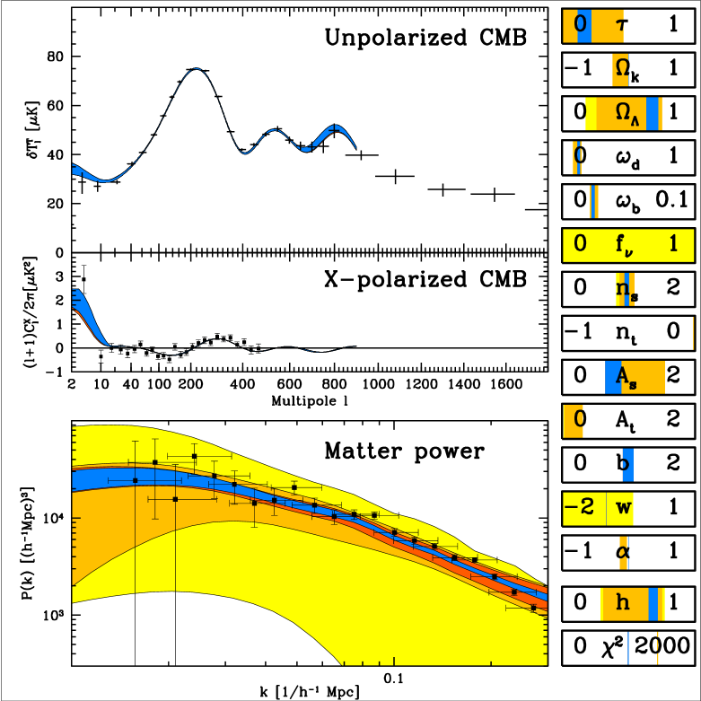
Figure  3.: Summary of observations and cosmological models taken from the combined analysis of WMAP and SDSS data  [?]. Data points are for unpolarized CMB experiments combined (top; Appendix A.3 details data used) cross-polarized CMB from WMAP (middle) and Galaxy power from SDSS (bottom). Shaded bands show the 1-sigma range of theoretical models from the Monte-Carlo Markov chains, both for cosmological parameters (right) and for the corresponding power spectra (left). From outside in, these bands correspond to 1.) WMAP with no priors; 2.) adding the prior of zero contribution from neutrinos $f_{\nu}=0$, and a cosmological constant $w=-1$, 3.) adding the priors $\Omega_{k}=0$ (flat universe), negligible gravity wave contribution $r=0$ and power law primordial spectra $\alpha=0$; and finally adding the SDSS information, respectively. These four bands essentially coincide in the top two panels, since the CMB constraints were included in the fits. Note that the $\l$-axis in the upper two panels goes from logarithmic on the left to linear on the right, to show important features at both ends, whereas the $k$-axis of the bottom panel is simply logarithmic.

Any observational comparison based on the structure formation in the universe necessarily depends on the assumed initial conditions describing the primordial seed perturbations of the perturbed universe. What has been remarkable is the extent to which recent cosmological observations have been consistent with and, in certain cases, even vindicated the standard assumptions. Besides, the entirely theoretical motivation of the paradigm of inflation, the assumption of Gaussian, random adiabatic scalar perturbations with a nearly scale invariant power is also arguably the simplest possible choice for the initial perturbations.

Table 2.: The current estimates of a selected set of cosmological parameters obtained from the CMB anisotropy and LSS power spectrum measurement from SDSS and Ly-$\alpha$ [?]. The results assume a flat universe and a cosmological constant (constant equation of state $w=-1$). The second and third columns correspond to parameter estimates when the space of IC parameters is curtailed by imposing the assumptions of negligible gravity wave contribution $r=0$ and exact power law primordial spectra $\alpha=0$. The error bars quoted is the larger of the upper and lower error bars ($1\sigma$ equivalent). For upper bounds the $95$% CL is quoted. See  [?] for exact error bars at $1\sigma$, $2\sigma$ and $3\sigma$ equivalent confidence levels.

Parameter	Priors ($\Omega_{K}=0$, $w=-1$)	+priors ($r=0$)	+priors ( $\alpha=0$)
$10^{2}\omega_{b}$	$2.42\pm 0.12$	$2.33\pm 0.09$	$2.31\pm 0.09$
$\Omega_{m}$	$0.27\pm 0.037$	$0.28\pm 0.022$	$0.3\pm 0.04$
$h$	$0.72\pm 0.037$	$0.71\pm 0.02$	$0.694\pm 0.03$
$\tau$	$0.14\pm 0.049$	$0.163\pm 0.04$	$0.133\pm 0.05$
$\sigma_{8}$	$0.9\pm 0.034$	$0.9\pm 0.03$	$0.89\pm 0.03$
$n_{s}$	$0.97\pm 0.023$	$0.98\pm 0.02$	$1.00\pm 0.03$
$10^{2}\alpha$	$-0.57\pm 1.2$	$-0.3\pm 1.1$	fixed
$r$	$<0.45$	fixed	fixed

In a simple power law parametrization of the primordial spectrum of density perturbation ($|\delta_{k}|^{2}=Ak^{n_{s}}$), the scale invariant spectrum corresponds to $n_{s}=1$. Recent estimation of (smooth) deviations from scale invariance favor a nearly scale invariant spectrum  [?]. Current observations favor a value of $n_{s}=0.98\pm 0.02$ (99.9%CL) which are consistent with a nearly scale invariant power spectrum. The current combined CMB and LSS data is good enough to constrain the ‘running’ of the spectral index, $\alpha={\rm d}n_{s}/{\rm d}\ln k=0.003\pm 0.01$ (99.9%CL). These results are remarkably consistent with the generic predictions of the simplest models of inflation. The power in the CMB temperature anisotropy at low multipoles ($l\mathrel{\hbox to0.0pt{\lower 4.0pt\hbox{\hskip 1.0pt$\sim$}\hss}\raise 1.0pt\hbox{$<$}}60$) first measured by the COBE-DMR  [?] did indicate the existence of correlated cosmological perturbations on super Hubble-radius scales at the epoch of last scattering, except for the (rather unlikely) possibility of all the power arising from the integrated Sachs–Wolfe effect along the line of sight. Since the polarization anisotropy is generated only at the last scattering surface, the negative trough in the $C_{l}^{\rm TE}$ spectrum at $l\sim 140$ (that corresponds to a scale larger than the horizon at the epoch of last scattering) measured by WMAP seals this loophole, and provides an unambiguous proof of apparently ‘acausal’ correlations in the cosmological perturbations  [?]. Inflation is the most promising causal explanation for the generation of these ‘acausal’ correlations. Further, the negative power in $C_{l}^{\rm TE}$ is a trademark of the adiabatic scalar metric perturbations that is also a generic prediction of the simplest models of inflation.

Other than some anomalies reported regarding the recent WMAP results (see below), the CMB anisotropy maps (including the WMAP non-gaussianity analysis carried out by the WMAP team  [?]) have been found to be consistent with a statistically isotropic, Gaussian random field. This assumption is theoretically motivated by inflation  [?]. The Gaussianity of the CMB anisotropy on large angular scales directly implies Gaussian primordial perturbations  [?].

Finally, the most interesting and robust constraint obtained is that on the spatial curvature of the universe. The combination of CMB anisotropy, LSS and other observations can pin down the universe to be spatially flat, $\Omega_{\rm K}=-0.02\pm 0.02$. These results are further tightened when combined with the constraints from high red-shift supernova (SN Ia). The connection between the geometry of space and the precise location of acoustic peaks leads to the widespread belief that the CMB data from WMAP alone can measure $\Omega_{\rm K}$ precisely. However, the present CMB anisotropy from the WMAP spectrum alone constrains the curvature rather weakly $-0.4\mathrel{\hbox to0.0pt{\lower 4.0pt\hbox{\hskip 1.0pt$\sim$}\hss}\raise 1.0pt\hbox{$<$}}\Omega_{\rm K}\mathrel{\hbox to0.0pt{\lower 4.0pt\hbox{\hskip 1.0pt$\sim$}\hss}\raise 1.0pt\hbox{$<$}}0.1$. This is due to the degeneracy $\Omega_{\rm K}$ with the Hubble constant, $h$ and the age of the universe, $t_{0}$. Even reasonably weak priors, $h>0.5$ or $t_{0}>12\,\,{\rm Gyr}$ tightens the constraint on $\Omega_{\rm K}$ significantly.

The current constraints on curvature density eliminates one of the three currently important players in eq. (2) leading to $\Omega_{\rm m}+\Omega_{\Lambda}\approx 1$. The physical origin and nature of $\Omega_{\Lambda}$ is one of the major challenges of present cosmology. The simplest parametrization of $\Omega_{\Lambda}$ as pure vacuum energy density with an equation of state $w=-1$ is consistent with all the observations  [?]. This conclusion appears to hold for the combination of CMB and LSS data in analyses where the equation of state is allowed to vary with red-shift  [?,?].

4. Discussion

Despite the precision of the cosmological parameter estimates, we do not know them ‘accurately’. It is clear from Table 2 that there are systematic differences in the median value depending on the choice of priors and the space of parameters. There are significant differences also due to the choice of the supplementary observational data sets used. The fact that the results differ when CMB anisotropy data are combined with different ‘complementary’ data sets also indicates that the other observational constraints are not as reliable as the CMB anisotropy  [?].

The dependence on the choice of the parameter space or the priors imposed on them simply arises due to the covariances (and degeneracies, therein) between parameters. Even imposing a uniform prior but on different parameter combination can make a difference to measurement of physical observables. For example, imposing uniform prior on the epoch of reionization $z_{\rm ion}$, instead of the optical depth $\tau$, tends to lower the estimate of $\tau$  [?,?]. Progress on new observational fronts would help resolve these issues by breaking the parameter degeneracies and eliminating/constraining extra parameters. For example, it is only very recently that the angular power spectrum of CMB polarization has been detected. The degree angular scale interferometer (DASI) has measured the CMB polarization spectrum over a limited band of angular scales ($l\sim 200$–440) in late 2002  [?]. The WMAP mission has also detected CMB polarization  [?]. WMAP is expected to release the CMB polarization spectra very soon. The results of much awaited CMB polarization spectrum from WMAP would be a crucial test of the early epoch of reionization and resolve some other degeneracies. Future experiments that target the $B$-mode polarization signature of gravity waves will be invaluable in pinning down the values of $r$, and consequently, in identifying the viable sectors in the space of inflationary parameters.

In principle, there is no well-defined procedure for selecting ‘the set’ of parameters. While there may be some consensus on the choice of cosmological parameters, the situation becomes murky when confronted with the parameters describing initial conditions (or, inflationary parameters). In the absence of an accepted early universe scenario (more narrowly, a favored model of inflation), it is difficult to a priori set up and justify the chosen space of initial conditions. The complex covariances between the cosmological and the initial parameters are sensitive to the parametrization of the space of initial spectra adopted. Efforts along these lines are further obscured by issues such as the applicability of the Occam’s razor to dissuade the extension of the parameter space of initial conditions. Such deliberations have been recently framed in the more quantitative language of Bayesian evidence to evaluate and select between possible parametrizations  [?]. However, this approach cannot really point to a preferred parametrization. A possible approach may be to maximize the likelihood over the space of initial conditions. This has been suggested in the context of the primordial power spectrum  [?]. A similar situation exists regarding the parametrization of the dark energy component.

The estimation of the parameters is only the first step. The challenge that lies ahead would be to connect them to physics. The physical origin and properties of the dark energy component is a complete mystery  [?]. While interpreting the cosmological constant as vacuum energy may be the simplest parametrization, it implies an extreme form of fine tuning. Quintessence field does alleviate the problem of fine tuning, but the scalar field does not appear to have any other reason for its existence (in contrast to the inflaton). So postulating a scalar field to explain one cosmological observation appears to be a theoretical overkill. The precise property of the cold dark matter remains an open problem. Eventually, direct detection and identification of the CDM particle candidates is perhaps needed. Meanwhile, cosmological observations pertaining to successful galaxy formation are beginning to put interesting constraints on the properties of the CDM  [?]. In particular, simulations using canonical ‘collision-less’ CDM appears to be at odds with the observations on small (sub Mpc.) scales. First, the substructure of CDM halos is predicted to be richer than observed. The number of small galaxies that are observed orbiting with a larger unit is less than expected. Second, the density profile at the centers of CDM halos is predicted to be ‘cuspier’ than observed. Addressing these issues is complex, since predictions come from large N-Body and hydrodynamic simulation which have their own limitations. At this time, we are still mired in uncertainty. Alternative variants to the collision-less CDM are under active investigation. They include possibilities such as self-interacting dark matter   [?], warm dark matter   [?], self annihilating dark matter  [?], massive black holes  [?], etc. There is an interesting phenomenology developing as sub-field of cosmology. It is not inconceivable that cosmological observations would pin down the properties of the CDM component well before any direct detection.

There could also be major surprises hidden in the current cosmological observations. After the recent release of the first year of WMAP data, anomalies such as the suppression of power in the lowest multipoles of the CMB anisotropy, possible breakdown of statistical isotropy (SI) and Gaussianity has attracted much attention. Tantalizing evidence for SI breakdown (albeit, in very different guises) has mounted in the WMAP first year sky maps, using a variety of different statistics. It was pointed out that the suppression of power in the quadrupole and octopole are aligned  [?], but this could be due to imperfect (galactic) foreground subtraction. Further ‘multipole-vector’ directions associated with these multipoles (and, some other low multipoles as well) appear to be anomalously correlated  [?,?]. There are indications of asymmetry in the power spectrum at low multipoles in opposite hemispheres  [?,?]. Possibly related, are the results of tests of Gaussianity that show asymmetry in the amplitude of the measured genus amplitude (at about $2$ to $3\sigma$ significance) between the north and south galactic hemispheres  [?,?]. Analysis of the distribution of extrema in WMAP sky maps has indicated non-Gaussianity, and to some extent, violation of statistical isotropy  [?]. These anomalies could be pointing to new physics with exciting cosmological ramifications and need to be addressed with specialized statistical measures  [?].

5. Summary

Observational cosmology has made impressive progress in recent years. We now have the ability to make precise measurements of cosmological parameters by including observational constraints from structure formation in the universe. While ability to make quantitatively ‘precise’ statements within a parameterized standard cosmology has improved remarkably, we still have far to go before we are ‘accurate’ in describing our cosmos. Observational cosmology has to first grapple with the physical interpretation of these precisely measured parameters!

REFERENCES

- [1] C L Bennett et al, Astrophys. J. Suppl. 148, 1 (2003)
- [2] A C Pope et al, Astrophys. J. 607 655 (2004) W J Percival et al, Mon. Not. R. Astron. Soc. 327, 1297 (2001)
- [3] M Tegmark et al, Astrophys. J. 606, 702 (2004)
- [4] D N Spergel et al, Astrophys. J. Suppl. 148, 175 (2003)
- [5] M Tegmark et al, Phys. Rev. D69, 103501 (2004)
- [6] U Seljak et al, preprint, astro-ph/0407372
- [7] N Bahcall, J P Ostriker, S Perlmutter and P J Steinhardt, Science 284, 1481 (1999)
- [8] R H Cyburt, B D Fields and K A Olive, Phys. Lett. B567, 227, (2003) D Kirkman et al, Astrophys. J. Suppl. 149, 1 (2003)
- [9] J L Tonry et al, Astrophys. J. 594, 1 (2003)
- [10] A G Reiss et al, Astrophys. J. 607, 665 (2004)
- [11] W L Freedman et al, Astrophys. J. 553, 47 (2001)
- [12] J R Bond, Theory and observations of the cosmic background radiation, in Cosmology and large scale structure, Les Houches Session LX, August 1993, edited by R Schaeffer, (Elsevier Science Press, 1996)
- [13] W Hu and S Dodelson, Ann. Rev. Astron. Astrophys. 40, 171 (2002)
- [14] R A C Croft, D H Weinberg, N Katz and L Hernquist, Astrophys. J. 495 44 (1998) P McDonald et al, preprint, astro-ph/0405013
- [15] G F Smoot et al, Astrophys. J. Lett. 396, L1 (1992)
- [16] E Komatsu, et al, Astrophys. J. Suppl. 148, 119 (2003)
- [17] A A Starobinsky, Phys. Lett. 117B, 175 (1982) A H Guth and S-Y Pi, Phys. Rev. Lett. 49, 1110 (1982) J M Bardeen, P J Steinhardt and M S Turner, Phys. Rev. D28, 679 (1983)
- [18] D Munshi, T Souradeep and A Starobinsky, Astrophys. J. 454, 552 (1995) D N Spergel and D M Goldberg, Phys. Rev. D59, 103001 (1999)
- [19] C R Contaldi, H Hoekstra and A Lewis, Phys. Rev. Lett. 99, 221303 (2003)
- [20] J M Kovac et al, Nature, 420, 772 (2002)
- [21] A Kogut et al, Astrophys. J. Suppl. 148, 161 (2003)
- [22] A Niarchou, A H Jaffe and L Pogosian, Phys. Rev. D69, 063515 (2004)
- [23] A Shafieloo and T Souradeep, Phys. Rev. D 70, 043523, (2004).
- [24] V Sahni and A Starobinsky, Int. J. Mod. Phys. D9, 373 (2000) T Padmanabhan, Phys. Rept. 380, 235 (2003) P J E Peebles and B Ratra, Rev. Mod. Phys. 75, 559 (2003)
- [25] J P Ostriker and P J Steinhardt, Science, 300, 1909 (2003)
- [26] D N Spergel and P J Steinhardt, Phys. Rev. Lett. 84, 3760 (2000)
- [27] P Colin, V Avila-Reese and O Valenzuela, Astrophys. J. 542, 622, (2000) P Bode, J P Ostriker and N Turok, Astrophys. J. 556, 93 (2001)
- [28] M Kaplinghat, L Knox and M S Turner, Phys. Rev. Lett. 85, 3335 (2000)
- [29] C Lacey and J P Ostriker, Astrophys. J. 229, 633 (1985)
- [30] M Tegmark, A de Oliveira-Costa and A Hamilton, D 68 123523 (2003).
- [31] C J Copi, D Huterer and G D Starkman, Phys. Rev. D 70 043515 (2004).
- [32] D J Schwarz et al, preprint astro-ph/0403353
- [33] C Park, Mon Not. Roy. Astron. Soc. 349, 313 (2004)
- [34] H K Eriksen et al, Astrophys. J. 605, 14 (2004)
- [35] F K Hansen, A J Banday and K M Gorski, preprint, astro-ph/0404206
- [36] H K Eriksen et al, Astrophys. J. 612, 64 (2004)
- [37] D L Larson and B D Wandelt, preprint, astro-ph/0404037
- [38] A Hajian and T Souradeep, Astrophys. J. Lett. 597, L5 (2003) A Hajian, T Souradeep and N Cornish, preprint, astro-ph/0406354