The impact of thermal gas in AGN jets on the low-frequency emission

We study the effect of non-relativistic, thermal matter in the jets of active galaxies (AGN) on the low-frequency non-thermal emission and the variability thereof. In matter-dominated jets, sizable quantities of gas should exist, in particular in the compression zones near the collision fronts that are an implicit ingredient of Fermi-type particle acceleration scenarios. Non-relativistic thermal gas in AGN jets noticably contributes to the optical depth at radio to infrared frequencies, and much less to the emission, with an efficiency that is strongly temperature-dependent. The observable flux of low-frequency emission is thus modulated by the temperature evolution of the thermal gas, and it can therefore display very complicated variability. For a particular particle energisation scenario we calculate the temperature evolution of the thermal plasma as well as the radiation transport of low-frequency emission, and thus derive simulated light curves at different frequencies and their typical correlation properties.

1 Introduction

Blazars, a sub-class of active galactic nuclei (AGN), are among the strongest known radiation sources in the universe. Observations show that they exhibit strong optical polarization, variability on all observable timescales, flat-spectrum radio emission from a compact core, and many of them emit the bulk of their luminosity in the form of $\gamma$-rays (e.g. Dermer & Gehrels 1995; Mukherjee et al. 1997). On account of these measurements it is usually argued that the $\gamma$-rays are produced in very compact regions within a relativistically moving system, the so-called jets, thus providing a strong Doppler amplification of the radiation. Often, the relativistic bulk motion can be directly observed as apparent superluminal motion of individual emission regions in the jets in sequences of VLBI observations of their radio emission. The Lorentz factors (and Doppler factors) thus derived are of the order of ten for general samples of AGNs (Vermeulen & Cohen 1994), but may be higher for AGNs showing prominent gamma-ray emission (e.g. Homan et al. 2002, 2003). The range of Lorentz factors prevalent at the time of gamma-ray emission, which presumably occurs before the emission region becomes visible at radio frequencies, is not known, but is likely higher than ten, if the bulk kinetic energy of the jets is the energy reservoir for the particle acceleration (see, e.g., Georganopoulos & Kazanas 2003). These conclusions are further supported by the absence of $\gamma-\gamma$ pair absorption and the violation of the Elliot-Shapiro relation (Elliot & Shapiro 1974) in several observed AGNs.

The unified model for active galaxies (Urry & Padovani 1995) assumes that a supermassive black hole is located in the center of a galaxy. The black hole supposedly accelerates plasma to high energies, while the surrounding host galaxy provides a steady inflow of matter, often assumed to be in the form of an accretion disk, to keep the system running for a long time. Above the accretion disk plasma is ejected in jets, which may reach lengths of several hundreds kpc (Begelman et al. 1984; Schlickeiser 2002).

Though thermal radiation can be observed from many AGN, it is usually associated with the accretion disk and the medium around it. The emission from the jets is generally assumed to be entirely non-thermal on account of the spectrum and the variability behaviour. Nevertheless, there may be thermal plasma in the jets, in which the dominantly radiating, energetic particles are embedded and confined.

In this paper we will study the effect of thermal matter in the jets on the low-frequency non-thermal emission and the variability thereof. We will do so in the framework of one particular model of particle acceleration, in which the energetic particles are provided by the isotropization of interstellar matter in the downstream region of a relativistic collision front (Pohl & Schlickeiser 2000, henceforth referred to as PS), though most of our treatment, and hence most of the results, are not restricted to the particulars of this scenario.

As we will see, the thermal gas will not necessarily manifest itself by its emission, but rather by its absorption. Both the emission and the absorption properties of thermal matter depend strongly on the temperature, and thus the problem at hand has two aspects. First, the radiation transport of low-frequency emission through thermal gas must be calculated, which is a function of the plasma temperature and density as well as of the spectrum of energetic particles. We then need to follow the temperature evolution of the thermal gas, which depends on the its emission and absorptions coefficients (and hence on its temperature), on the spectrum of energetic particles, and on possible wave damping. In this study we concentrate on continuum emission processes.

The spectrum of non-thermal particles obviously varies with time on account of the variability in the high-energy emission. Consequently the plasma temperature will vary, and so will the thermal absorption coefficient. The observable flux of low-frequency emission is thus modulated by the temperature evolution of the thermal gas, and it can therefore display very complicated variability behaviour, the study of which is the subject of this paper.

We first give a brief introduction into the PS model for active galactic nuclei (Sect. 2). After this, in Sect. 3 we discuss the radiation transport for a general non-thermal population of electrons in a warm electron-proton plasma. We present numerical absorption and emission coefficients for a generic situation (when this is possible) as well as for the PS model (when a generic treatment is not possible). In Sect. 5 we discuss the temperature evolution in a generic warm background plasma for different heating processes. The results of this analysis are independent of the non-thermal particle spectrum, so that they can easily be applied to other (non-)astrophysical situations.

In Sect. 4 and 5.5 we present numerical results for the PS model and demonstrate that only a few parameters actually influence the qualitative behaviour of a system. Section 5.5 emphasizes the limits of our calculations, while Sect. 6 connects these limits to free parameters in this situation.

2 The basic model

Pohl & Schlickeiser (2000) have studied the kinetic relaxation of particles that have traversed a parallel collision front from the upstream to the downstream region. This pick-up process occurs due to scattering off low-wavenumber plasma waves that the picked-up particles generate through streaming instabilities. The calculation describes the first half-cycle of the standard shock acceleration process for relativistic, collisionless flows. If the outflow plasma propagating through the jet is dense, the downstream region provides a target for the ultra-relativistic protons to interact with and produce radiation through various leptonic and hadronic emission channels. The predicted radiation properties resemble those of gamma-ray blazars and thus the model offers an attractive alternative to shock acceleration of electrons and subsequent Inverse Compton scattering.

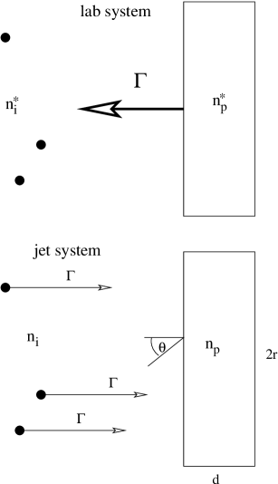
Figure 1: The geometry visualized for two systems of reference, the jet frame and the laboratory (host galaxy) frame, for which all quantities are indexed with an asterisk. We consider a single cloud of thermal proton-electron plasma with density $n_{\rm p}$, that is relativistically moving through the interstellar medium of the host galaxy with density $n_{\rm i}^{\ast}$. An observer would see radiation from the plasma cloud that is emitted at an angle $\theta$ with respect to its direction of motion.

The geometry of the system is shown in Fig. 1 for two systems of reference, the jet frame (without index) and the laboratory (host galaxy) frame, for which all quantities are indexed with an asterisk. In this report, we also use a third reference frame, the observer frame, which we use to calculate the observed evolution time. We will come back to this point later in this section. We consider the jet to consist of individual clouds of thermal proton-electron plasma, that are relativistically moving through the interstellar medium of the host galaxy. Here we discuss the interactions of one such cloud with temperature $T$, density $n_{\rm p}$, and as a simple approximation for its spatial extent and form a cylindrical disk with radius $r$ and thickness $d$. We emphasize that we treat the swept-up matter as a simple collection of particles, which is in accordance with the earlier model by Pohl & Schlickeiser (2000), and unlike the fluid treatment common to shock acceleration physics (Schlickeiser 2002). As a consequence, there is no relation between the two quantities $n_{p}$ and $n_{i}$, and the Rankine-Hugoniot conditions do not apply.

The Lorentz transformation between the two frames of reference gives the relations $n_{\rm i}=\Gamma n_{\rm i}^{\ast}$ and $n_{\rm p}^{\ast}=\Gamma n_{\rm p}$ with a relative Lorentz factor of $\Gamma$. The swept-up particles are of high energies in the instantaneous downstream (jet) frame and are quickly isotropized (Pohl & Schlickeiser 2000). Momentum conservation causes the system to decelerate, while internal processes produce a broad distribution of primary protons, $N_{\rm p}(\gamma_{\rm p})$, and secondary electrons, $N_{\rm e}(\gamma_{\rm e})$, which are more important than primary electrons for the parameters of interest. Unless noted otherwise, all relevant expressions use cgs units, all particle spectra $N_{\rm x}$ are taken per unit volume and all equations and formulae are taken in the instantaneous jet frame.

The isotropization of the swept-up particles effects a momentum transfer from the interstellar medium particles to the jet. Therefore, the jet decelerates and the Lorentz factor of the jet, $\Gamma$, is a function of time. It follows the equations (Pohl & Schlickeiser 2000)

$$\dot{\Gamma} = -\frac{\pi r^{2}n_{i}^{\ast}cm_{\rm p}}{M(t)}(\Gamma^{2}-1)^{3/2}$$ (1)

$$M(t) = V\sum_{\rm x=e,p}\int_{1}^{\infty}d\gamma\ m_{\rm x}\,\left(n_{b}+\gamma\,N_{\rm x}(\gamma,t)\right)$$ (2)

where $M(t)$ is the total mass of the compact plasma, which in turn depends on the differential number density of the energetic particles, $N(\gamma)$. Such gradual deceleration has been directly observed in the case of the micro-quasar XTE J1550-564 (Corbel et al. 2002).

The Lorentz factors observed in astrophysical sources vary greatly depending on the source class and the measured velocity indicator. While in gamma-ray burst (GRBs) they may reach values of several hundreds, the Lorentz factors in AGN jets are usually only of the order of ten, if deduced from measurements of superluminal motion, but may be higher for $\gamma$-ray-bright blazars. For TeV-blazars the radiation modeling often also requires significantly higher Lorentz (and Doppler) factors (e.g. Konopelko et al. 2003). However, gamma-ray emission is presumed to occur before the emission zone becomes visible at radio frequencies, and the corresponding Lorentz factor should thus be very much higher than ten, if the bulk kinetic energy of the jets is supposed to be the source for particle acceleration. Additionally, the physics of jet formation, and therefore the Lorentz factors involved with this process are not understood, but considering the supposedly extreme conditions near a black hole, it is highly possible that the particles which are ultimately injected into the jet initially possess similarly high velocities. For this reason, we assume an initial Lorentz factor $\Gamma_{0}=300$. We would like to point out that our results are only parametrically dependent on this choice.

In the instantaneous jet frame the differential number density of protons and electrons follows the evolution equation

$$\frac{\partial N}{\partial t}=\dot{N}-\frac{\partial}{\partial\gamma}\left(\dot{\gamma}N(\gamma)\right)-\frac{N(\gamma)}{T_{\rm c}}$$ (3)

where $T_{\rm c}$ is the timescale for particle losses by escape or decay, $\dot{\gamma}$ represents continuous energy losses, and $\dot{N}$ is the injection or production rate of new particles. As initial condition at the time $t=0$, when the jet Lorentz factor is $\Gamma=\Gamma_{0}$, we assume that there are no energetic particles in the jet, $N(\gamma)=0$.

In the default configuration the background plasma sweeps up protons from the interstellar matter, while electrons are produced in inelastic collisions in the system. The differential proton source density in the co-moving frame is (Pohl & Schlickeiser 2000)

$$\dot{N}={{c\,n_{\rm i}^{\ast}}\over d}\sqrt{\Gamma^{2}-1}\;\delta(\gamma-\Gamma)$$ (4)

while the (secondary) electron production proceeds through the reaction chain

$$p+p \rightarrow \pi^{\pm}+X$$ (5)

$$\pi^{\pm} \rightarrow \mu^{\pm}+\nu$$ (6)

$$\mu^{\pm} \rightarrow e^{\pm}+2\nu,$$ (7)

and is calculated numerically to properly account for the pion multiplicity spectrum in reaction (3). Here we use the Monte Carlo model DTUNUC (V2.2) (Möhring & Ranft 1991; Ranft et al. 1994; Ferrari et al. 1996a; Engel et al. 1997), which is based on a dual parton model (Capella et al. 1994). This MC model for hadron-nucleus and nucleus-nucleus interactions includes various modern aspects of high-energy physics and has been successfully applied to the description of hadron production in high-energy collisions (Ferrari et al. 1996b; Ranft & Roesler 1994; Möhring et al. 1993; Roesler et al. 1998).

The particle losses are diffusive escape (protons and electrons), neutron escape following $\hbox{p+p}\rightarrow\hbox{n+X}$ reactions and pair annihilation (electrons and positrons),

$$T_{\rm esc}=1.67\cdot 10^{-19}\ \frac{d^{2}\,\Gamma\,n_{i}^{\ast}}{\beta\sqrt{n_{\rm p}}}\quad\hbox{sec}$$ (8)

$$T_{\rm neu}=3\cdot 10^{15}n_{\rm p}^{-1}\left<\exp\left(-\frac{L}{\gamma\,2.7\cdot 10^{13}\ {\rm cm}}\right)\right>^{-1}\quad\hbox{sec}$$ (9)

$$T_{\rm ann}^{-1}=\frac{3c\sigma_{T}n_{\rm p}}{8(\gamma+1)\sqrt{\gamma^{2}-1}}\times$$ (10)

$$\left[(\gamma+4+\gamma^{-1})\log(\gamma+\sqrt{\gamma^{2}-1})-\beta(\gamma+3)\right]\quad\hbox{sec}^{-1}$$

$$\frac{1}{T_{\rm c,tot}}=\sum_{i}\frac{1}{T_{\hbox{c,}i}}.$$ (11)

For all relevant cases the exponential in eq. 9 (where $L$ is the distance to the plasma cloud boundary) can be approximated by 1 (Pohl & Schlickeiser 2000). We approximate the continuous losses by

$$-\dot{\gamma}_{\rm el,p} = 3.75\cdot 10^{-16}\ n_{\rm p}\,\frac{\gamma}{\sqrt{\gamma^{2}-1}}\quad\hbox{sec}^{-1}$$ (12)

$$-\dot{\gamma}_{\rm el,e} = 7.5\cdot 10^{-13}\ n_{\rm p}\,\frac{\gamma}{\sqrt{\gamma^{2}-1}}\quad\hbox{sec}^{-1}$$ (13)

$$-\dot{\gamma}_{\rm inel,p} = 7\cdot 10^{-16}\ n_{\rm p}\,\frac{(\gamma-1)^{2}}{\gamma+1}\quad\hbox{sec}^{-1}$$ (14)

$$-\dot{\gamma}_{\rm Sync} = 1.1\cdot 10^{-15}\ \frac{B^{2}}{m_{\rm e}c^{2}}\,\gamma^{2}\,\beta^{2}\quad\hbox{sec}^{-1}$$ (15)

$$-\dot{\gamma}_{\rm Brems} = 8\cdot 10^{-16}\ n_{\rm p}\,(\gamma-\gamma^{-1})\quad\hbox{sec}^{-1}.$$ (16)

Here the subscripts $el$ and $inel$ stand for elastic and inelastic processes, $Sync$ for synchrotron radiation and $Brems$ for Bremsstrahlung. The equations 12 and 13 are taken from Haug (1988), eq. 18, assuming a Coulomb logarithm of 25 and neglecting the last terms. This modification has been made to be consistent with eq. 48, while in Pohl & Schlickeiser (2000) a value of 20 is used. It does not affect the overall results in any visible way. Equation 15 is from Pacholczyk (1970), averaged over all emission directions. The inelastic energy losses, eq. 14 are a result of the model used to evaluate these processes (Capella et al. 1994). Finally, the Bremsstrahlung energy losses are taken from Hayakawa (1969) and Pohl & Schlickeiser (2000).

The timescales for particle losses are from Jauch & Rohrlich (1976) (eq. 10) and Pohl & Schlickeiser (2000) (eq. 8 and 9). The diffusive escape timescale used here is derived for the disk geometry under the condition $\hbox{r}\gg\hbox{d}$, which implies that effectively the charged particles will only escape through the top and bottom surfaces. The most important point here is the assumption that the energetic particles start diffusing outwards near the center of the jet plasma cloud. Depending on the Alfvén speed and the initial intensity of scattering waves this may be questionable (Vainio et al. 2004). We also want to emphasize that these equations have been derived under the assumption that the plasma is fully ionized and that the particle number is conserved. If this is not the case, the above equations have to be modified for ionization, recombination and pair production.

The free parameters of the model are specified in table 1 for a quick reference, where we also show the numerical values we have adopted as standard set of parameters in this paper. Whenever we modify one of these values, it is explicitely mentioned in the text.

parameter	default value
average magnetic field $B$	1 G
background plasma density $n_{\rm p}$	$5\cdot 10^{8}\hbox{cm}^{-3}$
interstellar matter density $n_{\rm i}^{\ast}$	$0.4\;\hbox{cm}^{-3}$
observer angle $\theta^{\rm obs}$	$0.1^{\circ}$
initial Lorentz factor $\Gamma_{0}$	300
disk height $d$	$3\cdot 10^{13}\;\hbox{cm}$
disk radius $r$	$10^{14}\;\hbox{cm}$
initial temperature $\rm T_{0}$	$10^{4}{\rm K}$

Table 1: Standard parameters used in this report unless noted otherwise. For the relation between the observer angle and the emission angle see Eq.17 and 18.

We have neglected all $e^{+}e^{-}$ annihilation processes, since we focus on the optical-to-infrared region where pair annihilation does not contribute.

All calculations in this analysis are made in the jet rest frame. For a comparison with observations, the photon spectra have to be transformed into the observer’s frame, which, depending on the cosmological redshift of the AGN in question, can be different from the host galaxy frame. For ease of exposition we will assume in the following treatment that the observer’s frame and the host galaxy frame are identical, as was done in Pohl & Schlickeiser (2000).

As a reminder we here list the relations between relevant quantities in the observer’s frame and the jet frame. While the observer’s frame is fixed, the jet frame is only the instantaneous rest frame of the jet plasma at the time considered. Since we are interested in the long-time evolution of a compact relativistic object moving along a straight line under a fixed aspect angle in the observer’s frame, we also need to consider that the corresponding aspect angle in the instantaneous jet frame is not constant, for the Doppler factor is changing with time.

$$\cos\theta^{obs} = \frac{\cos\theta+\beta_{\Gamma}}{1+\beta_{\Gamma}\cos\theta}$$ (17)

$$\cos\theta = \frac{\cos\theta^{obs}-\beta_{\Gamma}}{1-\beta_{\Gamma}\cos\theta^{obs}}$$ (18)

$$D = \frac{1}{\Gamma(1-\beta_{\Gamma}\cos\theta^{obs})}$$ (19)

$$\nu^{obs} = D\nu$$ (20)

$$I^{obs}(\nu^{obs}) = D^{3}I(\nu^{obs}/D)$$ (21)

$$dt^{obs} = dt/D$$ (22)

3 The radiation transport

3.1 The radiation transport equation

To calculate the emitted photon spectra $I_{\nu,0}$ for a given line-of-sight, it is required to know the emission coefficient $j_{\nu}$ and the absorption coefficient $\alpha_{\nu}$. These two quantities enter in the radiation transport equation (e. g. Rybicki & Lightman 1985),

$$\frac{dI_{\nu,0}}{d\tau}=S_{\nu}-I_{\nu,0}$$ (23)

via the source function $S_{\nu}=\sum_{i}j_{i}/\sum_{i}\alpha_{i}$ and the optical depth

$$\tau=\int_{0}^{s}\alpha\;dx\ .$$ (24)

The well-known general solution to this equation are for a path length of $s$

$$\begin{array}[]{llr}I_{\nu,0}(\tau)&=S_{\nu}\,\left[1-\exp(-\tau)\right]&\\ &=j_{\nu}\cdot s&\quad\hbox{for $\tau\ll$ 1}\hphantom{.}\\ &=S_{\nu}&\quad\hbox{for $\tau\gg$ 1}.\end{array}$$ (25)

In our calculations we have assumed that the radiation coefficients $j_{\nu}$ and $\alpha_{\nu}$ are independent of location, i.e. the supposedly cylindrical cloud of plasma in the jet is homogeneous, so that the optical depth reduces to

$$\tau_{s}=\alpha\cdot s$$ (26)

These expressions are the solution of the radiation transport equation for a single line-of-sight through the jet plasma. We still have to integrate over the entire emitting surface, as well as respecting the exact geometry of the system, since the photon path length is not constant over the apparent surface of the emission region. The total spectral power is then

$$P_{\nu}(\Omega) = \int dA(\Omega)\ I_{\nu,0}(\Omega)$$ (27)

with the apparent surface element $dA$ and the emission direction $\Omega$.

Since a real cloud of plasma will have a complicated (and generally unknown) geometry rather than the simple shape considered by Pohl & Schlickeiser (2000) and in this report, it may be sufficient to arrive at an approximate solution to Eq.27.

Let us start with the most simple approximation: we assume that the path length, $s$, is independent of the emission point both for the front surface, $A_{\rm f}$, and the side surface, $A_{\rm s}$. Then for the front surface

$$s_{f} \simeq d/\cos\theta,$$ (28)

and

$$P_{\nu,f}(\Omega) \simeq A_{f}\;\cos\theta\;I_{\nu,0}(d\theta)$$ (29)

$$\simeq \pi\,r^{2}\,\cos\theta\,S_{\nu}\,\left[1-\exp\left(-{{\alpha\,d}\over{\cos\theta}}\right)\right].$$ (30)

On account of the assumed thin-disk geometry, i.e. $d\ll r$, the contribution from the side surface is significant only for emission angles $\theta\approx\pi/2$. The choice of a thin disk for our system introduces an additional problem, for the photon path length between two opposite points on the side surface is not constant; we use $s\simeq r$ and obtain

$$s_{s} \approx r/\sin\theta,$$ (31)

and

$$P_{\nu,s}(\Omega) = A_{s}\;\sin\theta\;I_{\nu,0}(d\theta)$$ (32)

$$= 2\,d\,r\,\sin\theta\,S_{\nu}\,\left[1-\exp\left(-{{\alpha\,r}\over{\sin\theta}}\right)\right].$$ (33)

which turns out to be a fair approximation to the exact solutions of the problem, which are derived in appendix A.

A better approximation is afforded by a box geometry instead of the original cylinder. The side lengths would be $a=\sqrt{\pi}\,r$ to conserve the volume. If one assumes that the line-of-sight to the observer is in the plane of two of the side surfaces, Eq.27 can be solved exactly. The resulting expressions for the observable photon spectra are presented in appendix B. The box geometry turns out an excellent approximation to the exact solution for the initially assumed disk geometry, with a maximum error of 3% at $\theta=60^{\circ}$, while the simple constant-$s$ approach introduces an error of 20-30%.

3.2 The emission coefficients

In this report we consider two different contributions to the radiation processes, synchrotron emission and thermal bremsstrahlung (free-free emission). The bremsstrahlung coefficients for a quasineutral thermal hydrogen plasma are (Rybicki & Lightman 1985)

$$j_{br}=\frac{\sqrt{2}\,n^{2}\,\alpha\,\sigma_{T}\,\hbar\,c}{\pi^{3/2}}\sqrt{\frac{mc^{2}}{kT}}\,\ln\left({{2\,kT}\over{h\nu}}\right)\,\exp\left(-\frac{h\nu}{kT}\right)$$ (34)

$$\alpha_{br}=\frac{2\,n^{2}\,\alpha\,\sigma_{T}\,c^{3}}{(2\pi)^{5/2}\,\nu^{3}}\sqrt{\frac{mc^{2}}{kT}}\,\ln\left({{2\,kT}\over{h\nu}}\right)\left[1-\exp\left(-\frac{h\nu}{kT}\right)\right]\,.$$

   (35)

Figure 2: The absorption coefficients $\alpha$ for the free-free process and the synchrotron process for the jet model of Pohl & Schlickeiser (2000) with standard parameters (see table 1). We display the situation after one hour in the observer’s frame, at which time the plasma temperature is T$\approx 3\cdot 10^{4}\,$K. Apparently the system is dominated by free-free absorption.

Figure 3: The emission coefficients $j$ for the free-free process and the synchrotron process after one hour observed time for standard parameters, as in Fig.2. The free-free emission is only visible because of the Razin effect. For $n_{\rm p}=5\cdot 10^{8}\ {\rm cm}^{-3}$ the plasma frequency corresponds to $E_{\nu}\approx 8\cdot 10^{-7}\ {\rm eV}$, so we cover the entire valid energy spectrum.

The synchrotron radiation coefficients for an ensemble of electrons with differential number density $N(\gamma)$ can be calculated as (Rybicki & Lightman 1985)

$$j_{\rm sy} = \frac{1}{4\pi}\int_{1}^{\infty}d\gamma\;N(\gamma)\,p_{sy}(\nu)$$ (36)

$$\alpha_{\rm sy} = -\frac{1}{8\pi m\nu^{2}}\int_{1}^{\infty}d\gamma\;(\gamma^{2}-1)\,p_{sy}(\nu)\,\frac{\partial}{\partial\gamma}\left(\frac{N(\gamma)}{\gamma^{2}-1}\right)$$ (37)

with the spectral power per electron

$$p_{sy}(\nu)=\frac{\sqrt{3}e^{3}B}{mc^{2}}\,F\left(\frac{\nu}{\nu_{c}}\right)$$ (38)

where

$$\nu_{c}=\frac{3eB}{4\pi mc}\gamma^{2}\qquad\qquad F(x)\approx 1.8\;x^{1\over 3}\,\exp(-x)$$ (39)

In a dense plasma with plasma frequency $\nu_{\rm p}$ the spectral power is modified at low frequencies by the Razin effect (Rybicki & Lightman 1985; Crusius & Schlickeiser 1988) on account of the modified dispersion relation for electromagnetic waves. Then

$$p_{sy,Razin}(\nu)=\frac{p_{sy}(\nu R^{3/2})}{\sqrt{R}}$$ (40)

where

$$R=1+\left(\frac{\nu_{\rm p}\gamma}{\nu}\right)^{2}\qquad\qquad\nu_{\rm p}\simeq 9\cdot 10^{3}\sqrt{n_{\rm p}}\ {\rm Hz}.$$ (41)

The Razin effect creates a cutoff in the photon spectrum at low energies, whereas at high energies the emission spectrum is unchanged.

The radiation coefficients for the standard parameters (see table 1) in the jet model of Pohl & Schlickeiser (2000) are displayed in Fig.2 and Fig.3. The synchrotron coefficients are based on the numerically derived electron spectrum in the system after one hour of observed time, while the free-free radiation coefficients depend only on the temperature, which is approximately $3\cdot 10^{4}\ {\rm K}$ at this time. The kinematic of the pion and muon decays is unfavorable for the production of secondary electrons with an energy less than approximately 100 MeV. Thus, essentially only highly relativistic electron are generated. The energy loss rate below 300 MeV is dominated by Coulomb and ionization interactions, i.e. is independent of energy, so that in a steady-state spectrum the cooling tail towards lower energies would be flat. The synchrotron spectrum in Fig. 3 is correspondingly inverted.

Figure 4: Emitted photon spectra after one hour of observed time in the jet system for the standard parameters ($\theta^{\rm obs}\approx 0.1^{\circ}$, see table 1) and $T\approx 3\cdot 10^{4}\,$K. The thermal Bremsstrahlung dominates at low energies only because of the Razin-effect, which suppresses the synchrotron spectrum here.

Figure 5: Emitted photon spectra in the jet frame after one hour of observed time for different emission angles, based on an exact treatment of the geometry. For high $\theta^{\rm obs}$, the slow evolution of the synchrotron part of the spectrum has been reproduced.

The non-thermal emission spectra do not significantly change when we modify the parameters, except for an approximately linear dependence on the density of the interstellar medium, so the results displayed here are a good estimate in most situations. The free-free absorption, and to a smaller extent the emission, is strongly reduced in efficiency for higher temperatures. As we shall see later, the plasma temperature can rise from $T=3\cdot 10^{4}\,$K, which nearly is a lower limit, to $10^{9}\,$K or more. Modifying the temperature from $3\cdot 10^{4}\,$K to this value reduces the absorption coefficient by 7 orders of magnitude, which makes the free-free absorption less efficient than the synchrotron absorption. The temperature, for which both are approximately equal, is around $10^{8}\,$K.

It thus appears that the optical thickness is mostly dominated by free-free absorption, while the emission is dominated by either synchrotron radiation or bremsstrahlung, depending on the frequency. It is important to include the Razin effect in our calculations, for, without the Razin effect, the synchrotron emission coefficient would not have a cut-off at low frequencies, and free-free emission would be completely negligible.

An interesting possibility is that a synchrotron maser may operate in the jet plasma. Maser activity requires a negative absorption coefficient ($\alpha<0$), indicating that stimulated emission is more important than the spontaneous absorption. If the optical depth $\tau\ll-1$, the emitted photon intensity can be very high.

Crusius & Schlickeiser (1988) have shown that for the synchrotron process this is only possible when the electron spectrum has a slope of at least 2, i.e. the distribution function is inverted. The numerical calculations of the inelastic proton decay chain seem to indicate that this is not the case, at least in the energy regions covered in this report. The condition for synchrotron masering is $\alpha<0$, and since the evaluation of $\alpha$ requires an integration over the entire radiating particle distribution (eq. 37), this condition must be valid for a large energy interval, and a locally hard spectrum will not be sufficient for a maser to operate.

4 Simple photon spectra

In this section we discuss radiation spectra for a constant temperature with a view to understand the characteristic properties of the escaping low-frequency emission. After one hour of observed time, the temperature is $T\approx 3\cdot 10^{4}\ {\rm K}$.

Photon spectra calculated on the basis of the exact disk geometry are presented in Fig. 4. The spectrum can be separated in an optically thick region and an optically thin region. The optical depth itself is dominated by the free-free absorption process. The emission process is dominated by the synchrotron process, for which the Razin effect causes a drop off below a certain photon energy, so that at very low frequencies the free-free emission becomes visible.

The spectra shown here are calculated in the jet frame, and thus they need to be transformed in the observer system for a comparison with data. For blazars, this would result in a frequency shift by about two orders of magnitude, so the turn-over frequency, at which the emission transitions from optically thick to optically thin conditions, would be located in the near-infrared.

Next, we calculate the emitted photon spectra for different observation angles $\theta^{\rm obs}$ and show typical results in Fig.5. For very small aspect angles $\theta^{\rm obs}\leq 1^{\circ}$, the jet system appears to rapidly evolve; in fact $\Gamma\approx 270$ after one hour of observed time. This value is still very high compared to typical Lorentz factors of 10, but one should note that it takes months for an outburst to become visible at radio frequencies, where most measurement of jet velocity are made.

The characteristic aspect of these spectra is the presence of both the thermal and the synchrotron components of the spectrum. Variations on the high-frequency part of the spectrum, most notably a shift of the turn-over frequency, are visible, which result from the different aspect in the jet frame, i.e. the different optical depth for a frontal and side view of the emission region in the jet frame.

For larger observation angles ($\theta^{obs}>1^{\circ}$), the system evolves much slower, so that $\Gamma\approx\Gamma_{0}$ after a single hour.

5 The evolution of the temperature

Throughout this paper we have assumed that LTE is valid, that the jet plasma is always non-relativistic, and that the electron and proton components have the same temperature, i.e. the internal equilibration processes are faster than the energy exchange with the environment.

5.1 The cooling process

As we have seen, the temperature of the jet plasma is a decisive parameter for the radiation yield at low frequencies. The plasma is subjected to a number of heating and cooling processes, and therefore the temperature will not remain constant. We use a balance equation to follow the variations of the plasma temperature,

$$\dot{T}=\frac{1}{n_{\rm p}k}(\gamma-1)(\dot{\epsilon}-\Lambda)\ ,$$ (42)

with the adiabatic index $\gamma$ (=5/3 for a non-relativistic hydrogen gas), the heating rate, $\dot{\epsilon}$, and the cooling rate, $\Lambda$. For the cooling rate we use an analytical approximation (see fig. 6) of the standard interstellar cooling function (Dalgarno & McCray 1972; Raymond et al. 1976).

$$\Lambda=\left(10^{-22}\ \hbox{erg cm}^{-3}\hbox{ s}^{-1}\right)\,n_{\rm p}^{2}$$

$$\hphantom{\Lambda=}\times\,\left\{\begin{array}[]{rll}2.3\cdot 10^{-5}&T^{1.1}&\mbox{for }\ 10^{2}\leq T\leq 10^{4}\\ 0.64&T^{0.55}&\mbox{for }\ 10^{4}\leq T\leq 10^{5}\\ 3.6\cdot 10^{5}&T^{-0.6}&\mbox{for }\ 10^{5}\leq T\leq 4\cdot 10^{7}\\ 1.6\cdot 10^{-3}&T^{0.5}&\mbox{for }\ T\geq 4\cdot 10^{7}\end{array}\right.$$ (47)

where the temperature, $T$, is in units of Kelvin. The error introduced by this approximation is not significant, for other uncertainities such as the real geometry have a much greater impact on the final results. A possible exception is the jump at $T\simeq 10^{4}\ {\rm K}$ that results from electron-impact excitation and ionization of H i, but may be modified here on account of the collisional excitation and ionization by the energetic particles.

Figure 6: The approximated cooling function according to Eq.47.

5.2 The Coulomb heating process

The heating rate is more difficult to calculate, since there are several concurring contributions. For a completely ionized plasma, the heating rate from elastic Coulomb scattering of a distribution of suprathermal electrons or protons, $N(\gamma)$, in a thermal plasma of temperature $T$ is given by (Butler & Buckingham 1962; Haug 1988)

$$\dot{\epsilon}=\int_{1}^{\infty}d\gamma\;N(\gamma)\,\frac{3}{2\beta}\,\sigma_{T}\,m_{\rm e}c^{3}\,n_{\rm p}\,\ln{\Lambda}$$ (48)

where $\ln\Lambda\approx 25$ is the Coulomb logarithm. This expression is valid for protons and electrons (this follows from Eq.13 and 12), so that usually the non-thermal particles with the greatest number density dominate this heating process. In most practical situations in our model, this is the secondary-electron population.

If only relativistic particles are considered, $\gamma\gg 1$ and $\beta\simeq 1$; then the heating rate scales linearly with the total number density of high energy particles, $N_{\rm tot}$.

$$\dot{\epsilon} \simeq \frac{3}{2}\,\sigma_{T}\,m_{\rm e}c^{3}\,n_{\rm p}\,N_{\rm tot}\,\ln{\Lambda}$$ (49)

5.3 The synchrotron heating process

Heating is also effected by absorption of non-thermal emission. In our case, the dominant process is free-free absorption of synchrotron photons. The synchrotron absorption coefficient is usually small compared to the free-free absorption coefficient, and hence the emitted radiation is almost exclusively absorbed by the free-free process. The heating rate can be calculated as an integral over the deficit in total luminosity caused by the absorption.

$$\dot{\epsilon}=\frac{1}{V}\int_{0}^{\infty}d\nu\left(4\pi Vj_{\nu}-2\pi\int d\theta\ P_{\nu}(\Omega)\right)$$ (50)

The spectral power, $P_{\nu}(\Omega)$, is given by Eq.27 and strongly dependent on the emission angle, thus necessitating the integral over $\theta$. In appendix A we will discuss ways to arrive at approximate solutions to $P_{\nu}(\Omega)$ with various degrees of accuracy.

5.4 Comparing both heating processes

It may be useful to identify parameters, for which Coulomb heating is always more efficient than heating by absorption, in which case solving Eq.50 would not be necessary. For that purpose, we neglect the Razin effect, for the very low-frequency photons do not significantly contribute to the total heating rate. We also note that the optical depth is strongly dependent on frequency, thus effectively dividing the spectrum at the turn-over frequency $\nu_{+}$, for which $\tau=1$, in a low-frequency part at $\nu\leq\nu_{+}$, in which essentially all photons are absorbed, and a high-frequency part at $\nu\geq\nu_{+}$, in which essentially all photons escape.

We have noted before that free-free absorption is generally more efficient than synchrotron absorption. The turn-over frequency $\nu_{+}$ is determined by the absorption coefficient (Eq.35) and the path length $s$. Setting the logarithmic term to the constant value $L$ we find in the limit $h\nu\ll kT$

$$\nu_{+} = n_{\rm p}\,\sqrt{\frac{2\,\alpha\,\sigma_{T}\,\hbar\,c}{(2\pi)^{3/2}\,m_{\rm e}}}\,\left(\frac{mc^{2}}{kT}\right)^{3/4}\,\sqrt{s}\,\sqrt{L}$$

$$\approx (10^{11}\,\hbox{\rm Hz})\left(\frac{n_{\rm p}}{\rm 10^{9}\,cm^{-3}}\right)\sqrt{\frac{s}{\rm 10^{14}\,cm}}\sqrt{\frac{L}{\rm 10}}\left(\frac{T}{\rm 10^{6}\,K}\right)^{-{3\over 4}}$$

With these approximations eq. 50 reduces to a much simpler form. Using eq. 36 and changing the order of integration we obtain

$$\dot{\epsilon} \leq \int_{0}^{\nu_{+}}d\nu\;4\pi j_{\nu}$$ (52)

$$= \int_{1}^{\infty}d\gamma\;N(\gamma)\int_{0}^{\nu_{+}}d\nu\;p_{sy}(\nu)=\int_{1}^{\infty}d\gamma\;N(\gamma)\,f(\gamma)_{sy}.$$ (53)

This integral has the same mathematical form as that in Eq.48 and Eq.49, implying that is may be sufficient to compare the weight functions for the heating processes, $f$.

For Coulomb heating by relativistic particles, the weight function, $f_{\rm el,e}$, follows directly from eq. 49,

$$f(\gamma)_{\rm el,e} \simeq 6\cdot 10^{-19}\,n_{\rm p}\quad{\rm erg\,cm^{3}\,s^{-1}}\,.$$ (54)

Since electrons and protons have the same weight functions, $f(\gamma)_{\rm el,e}=f(\gamma)_{el,p}$, this applies to protons as well, which are usually less numerous that electrons and therefore won’t dominate the overall heating process.

The synchrotron weight function is more difficult, for the integral over $\nu$ in Eq.53,

$$f(\gamma)_{\rm sy} = \int_{0}^{\nu_{+}}d\nu\;p_{sy}(\nu)$$ (55)

$$= 1.8\,\frac{\sqrt{3}e^{3}}{mc^{2}}\,B\int_{0}^{\nu_{+}}d\nu\ \left(\frac{\nu}{\nu_{c}}\right)^{1/3}\exp(-\frac{\nu}{\nu_{c}})$$

requires a numerical treatment for general $\nu_{+}$. However, an approximate solution can be derived. For that purpose we compare the electron energy loss rates for synchrotron emission (Eq.15) and Coulomb scattering (Eq.13). For electron Lorentz factors, $\gamma$, smaller than the critical value

$$\gamma_{-} = \max(1,g(n_{p},B))$$ (56)

$$g(n_{p},B) = \sqrt{682\frac{n}{B^{2}}m_{\rm e}c^{2}}\approx 0.024\left(\frac{n_{\rm p}}{\rm cm^{3}}\right)^{1/2}\left(\frac{B}{\rm G}\right)^{-1}\ ,$$ (57)

the electrons lose more energy by Coulomb scattering than by synchrotron radiation. This implies that Coulomb interactions are the dominant heating process, whatever the optical depth of the jet plasma. Only at Lorentz factors $\gamma\geq\gamma_{-}$ will the electrons dump a significant fraction of their energy into the radiation field. At these energies, the electrons will mainly radiate at frequencies $\nu\geq\nu_{-}$, where

$$\nu_{-}=(2.2\cdot 10^{13}\,{\rm Hz})\,\left(\frac{n_{\rm p}}{\rm 10^{9}\,cm^{-3}}\right)\left(\frac{B}{\rm G}\right)^{-1},$$ (58)

i.e. under optically thin conditions for the standard parameters (see table 1). So

$$\qquad\nu_{-} \gg \nu_{+}$$

$$\Leftrightarrow\left(\frac{T}{\rm 10^{4}\,K}\right)^{3\over 4} \gg 0.14\ \sqrt{\frac{s}{\rm 10^{14}\,cm}}\,\sqrt{\frac{L}{\rm 10}}\,\left(\frac{B}{\rm G}\right)$$ (59)

which means that only a small fraction of the synchrotron emission will be absorbed by the plasma, and thus Coulomb heating should always be more efficient than heating by absorption. A careful evaluation of Eq.55 using a Taylor expansion in $\nu_{+}\ll\nu_{c}$ indicates that the numerical factor on the RHS of Eq.59 should be closer to unity, but, on the other hand, that equation does not consider the heating by energetic protons. We may therefore conclude that synchrotron heating can be neglected, if the condition (59) is met.

5.5 The balance of heating and cooling

The evolution of the temperature is closely tied to the evolution of the heating and cooling rates. For a homogeneous interstellar medium the system will tend to attain a quasi-steady state. Consequently, the heating rates rise with time until they reach an asymptotic value. The temperature then evolves until the cooling balances the heating.

The cooling rate is a strong function of the temperature, with a huge jump at $10^{4}\,$K as the dominating feature at low temperatures (see fig.6). To reach higher temperatures, the heating rate must be large enough to compensate the hydrogen cooling, or the system will stay at $10^{4}\,$K, where the ionization fraction of hydrogen may be low, which results in an even lower turn-over frequency, so that the entire emission may be optical thin. Additionally, it is likely that under the conditions prevailent in the jet plasma, the temperature dependence of the ionization fraction is weaker than in the LTE calculations of Dalgarno & McCray (1972) and Raymond et al. (1976), thus causing a slower rise of the cooling curve. Nevertheless, the system will have a stable region around $10^{4}\,$K for a wide range of heating rates.

When the heating rate becomes larger than the maximum of the cooling function at $10^{5}\,$K, the temperature will increase to more than $10^{8}\,$K, beyond which bremsstrahlung cooling may again balance the heating. Extrapolating the cooling function to temperature $T\gtrsim 10^{8}\,$K is problematic, though, for one quickly arrives at relativistic temperatures, $kT\gtrsim m_{\rm e}c^{2}$, at which most of our assumptions and formulae are no longer valid. At these temperatures, it is especially required to include pair production into our equations, which increases the particle number in the background plasma while reducing the amount of energy available for the individual particle, thus efficiently limiting the temperature of the system. In addition, the concept of a stable isotropic Maxwell-Boltzmann distribution is not well justified in these regions (Stepney 1982).

For the standard parameters (see table 1), this overheating does not happen (see fig. 7), while for $n_{i}^{\ast}=0.8\;\hbox{cm}^{-3}$ the heating processes are too strong to keep the temperature non-relativistic. The Fig. also demonstrates that the synchrotron contribution to the heating rate is quite small; numerical evaluations show that this process contributes about 10 % of the Coulomb heating rate, which is in good agreement with our estimate in the preceding section. Finally, the asymptotic cooling is a direct result of the deceleration of the system, which decreases the number of swept up particles (eq. 4). At $t=0$, when there are no non-thermal particles present, the heating rates equal zero, and the system usually cools down to the stable point at $10^{4}\,$K. It is possible to prevent this with a careful choice of initial parameters, which results in stable temperatures of $T=10^{8}\,$K.

Figure 7: The temperature as a function of time for the standard parameters as well as $n_{\rm i}^{\ast}=0.8\;\hbox{cm}^{-3}$, for which the temperature becomes larger than $10^{9}\,$K, where our model is invalid.

6 Results

6.1 Modifying the initial parameters

In the last sections we have seen that the temperature of the background plasma can be used to estimate the stability of our model. For this reason, we have made a parameter study to approximate the regions in which we get reliable results. We have discovered four different regions: cold ($T\leq 10^{4}\,$K), warm ($10^{4}\,$K$\leq T\leq 10^{5}\,$K), hot ($10^{8}\,$K$\leq T\leq 10^{9}\,$K) and forbidden ($T>10^{9}\,$K). The region between $10^{5}\,$K and $10^{8}\,$K is unstable, which is a result of the specific form of the cooling function. The region between $10^{8}$ and $10^{9}\,$K is stable only for very specific initial parameters, as outlined in the last section.

The particle number densities $n_{\rm p}$ and $n_{\rm i}^{\ast}$ strongly dominate the system; the different regions in the $n_{\rm p}-n_{\rm i}^{\ast}$-plane for the standard parameters (see table 1) are displayed in Fig.8. Another parameter which determines the temperature evolution is the size of the system. It turns out that on account of the particle number sweep-up rate (eq.4), which is proportional to the sweep-up surface divided by the total volume of the system, only one of the size parameters really contributes to this point, which can be identified as the average optical path for a generic system. For the specific disk geometry, this parameter is identical to the thickness $d$; then for the standard parameters the boundary points are

$$d_{cold-warm} \approx 2.1\cdot 10^{13}\ \hbox{cm}$$ (60)

$$d_{warm-hot\ } \approx 4.1\cdot 10^{13}\ \hbox{cm}$$ (61)

Since the secondary electrons dominate the heating process (see Sect. 5.2), and their production rate can not be treated analytically, these results can not be derived from Fig. 8.

The initial Lorentz factor $\Gamma(t=0)$ modifies the interstellar matter density in the jet frame, $n_{\rm i}=\Gamma(t)n_{\rm i}^{\ast}$. This in turn modifies the number of particles in the system and therefore the heating rate by elastic scattering. However, it does not modify the form of the boundaries of temperature regions in the $n_{\rm p}-n_{\rm i}^{\ast}$-plane, but only their location. To demonstrate this, in fig. 8 we also display the temperature regions for $\Gamma_{0}=600$.

The observer angle $\theta^{\rm obs}$ only modifies the observed time required for the system to evolve, so the asymptotic behaviour remains unchanged. The magnetic field strength $B$ has practically no influence on the temperature, since the synchrotron heating process is negligible.

As mentioned earlier, by modifying the initial temperature $T_{0}$ together with the interstellar matter density $n_{\rm i}^{\ast}$, we are able to establish stable ’hot’ temperatures. In most cases, however, the initial temperature will not modify the system.

Figure 8: The three qualitatively different temperature regions as a function of the particle densities and the standard parameters ($T_{0}=10^{4}\,{\rm K}$). The dotted lines are for $\Gamma_{0}=600$.

From this we conclude that our model is stable only on a rather small region in the initial parameter space. In this case, there are three asymptotically stable temperature regions, and it may be possible to fix some of these parameters by observations. In all other cases, the initial assumption of a non-relativistic thermal component in the jets breaks down, although the sweep-up mechanism itself remains valid.

6.2 Time-dependent variations of free parameters

In a real situation the extragalactical matter density $n_{\rm i}^{\ast}$ is not constant over long timescales and distances. The plasma in the jet may cross dense clouds of hydrogen or enter a local fluctuation. For this reason we have investigated the temperature evolution under some simple modifications of our sweep-up rate.

First, we have considered a simple step in the ambient matter density,

$$\dot{N}_{cld} = \dot{N}(1+a\Theta(t_{1}-t)).$$ (62)

Such a situation may possibly be found when the jet leaves the immediate host galaxy and enter the intergalactic medium. In this case it is slightly easier to produce stable temperatures at $10^{8}\,$K, although this situation will still be quite rare. Generally, this modification simply produces a break in the temperature evolution.

Secondly, we have investigated the effect of local density fluctuations. We have studied a situation in which the system periodically passes through a dense cloud of material, that is embedded in low-density gas, where for a single period $\tau$ the sweep-up rate is

$$\dot{N}_{peak}(t) = \,\left\{\begin{array}[]{rl}a&\mbox{for }t<c\\ b&\mbox{for }c<t<\tau\end{array}\right.$$ (65)

with $a\gg b$ and $c$ the fraction of the period where the heating is strong. We have normalized these parameters in a way that the interstellar matter density averaged over a period is $n_{\rm i}^{\ast}$. Under this periodically peaked scheme, it is again easier to keep the system stable at $10^{8}\,$K without causing overheating as described in chapter 5.5.

6.3 Light curves and correlations

We have then calculated light curves for several different energies, which we present in Fig. 9 for the periodically peaked injection and the standard parameters. Unlike the other photon spectra presented in this report, these curves are taken in the observer frame, in which, on account of the deceleration of the jet, the frequency corresponding to a fixed jet-frame frequency varies with time, although the modification usually is small.

We see that the variability is visible, but that the average behaviour of the system remains unchanged. Additionally, the variability only affects the optical thick region, which is a result of temperature variations. In the optical thick region, we have $I\propto j/\alpha$ (eq. 25) and $\alpha\approx\alpha_{\rm thermal}$, which in turn causes $F_{\nu}$ to depend on the temperature. Since the heating rate is proportional to the total number of energetic particles, a sudden increase in this number causes a similar modification of the temperature of the jet plasma, which again modifies the optical thick emission. Because of $j\approx j_{\rm sy}$, the optical thin emission (see eq. 25) does not demonstrate a similar behaviour. For this reason our model is able to reproduce different variability in different freqnency bands.

Figure 9: Light curves for three different energies in the observer frame. Here we have adopted the periodic peak injection introduced in eq. 65 with the parameters $a/b=50$, a period of $\tau=1000\,{\rm s}$ observed time and $c=100\,{\rm s}$, i. e. 10% of the period time. Significant variations occur exclusively in the optical thick regime; the redshift of the source has been set to $z=0.5$.

Next, we have calculated correlation coefficients for this injection profile, using light curves in the observer frame between the infrared, optical and ultraviolet, from the plasma frequency up to a few 10 eV, with small and large distances between the considered frequencies.

It turns out that the lightcurves at different frequencies are almost perfectly correlated ($>0.9$), even if we compare free-free-dominated with synchrotron-dominated parts of the spectrum. To understand this behaviour, we first note that the electron distribution is dominated by the diffusive escape process (eq. 8), while the continuous losses are too inefficient. For high-energy electrons the particle spectrum is exclusively determined by the Lorentz factor of the jet, $\Gamma$. For this reason all light curves produced by the electrons are highly correlated with each other, even between the free-free and synchrotron processes, since the free-free emission depends on the temperature, which again is determined by the high-energy electrons, similar to the synchrotron emission. Given that the optically thin synchrotron emission shows only a very weak response to the variations in the injection rate, most of the correlation signal is presumably caused by the common secular trend in all light curves that is caused by the deceleration of the jet.

7 Possible corrections

In this section we briefly discuss possible further aspects of the problems investigated in this paper.

7.1 The electrostatic instability

Recently, Pohl et al. (2002) have investigated the electrostatic instability in a relativistic beam of electrons and protons and its impact on our model. Their conclusion was that the sweep-up spectrum effectively gets modified from a peak structure at $\gamma=\Gamma$ to a plateau distribution up to $\gamma=\Gamma$, while keeping the number of collected particles and the low-energy photon spectrum unchanged. The energy lost in this process may contribute to the heating of the background plasma, but there is no reliable estimate available of the exact amount of energy transferred. Observations hint that only a tiny fraction of the total energy lost by this mechanism can ever contribute to the heating.

Since this process in principle involves a huge amount of energy, it might dramatically change the evolution of the temperature. However, Pohl et al. (2002) have only considered the initial situation of a cold electron-proton beam penetrating cold thermal plasma. The presence of isotropic energetic particles should strongly reduce the growth rate of electrostatic turbulence, so that at least in a quasi-steady state heating by damping of electrostatic waves should be much less severe than suggested by the asymptotic energy loss of the incoming particle beam.

7.2 The initial conditions

Currently, our initial conditions assume that there are no non-thermal particles present. Although the mechanism responsible for creation and stability of the jets is not completely understood (Urry & Padovani 1995; Begelman et al. 1984), it is likely that there is no time zero, at which a plasma cloud is relativistically expelled without containing energetic particles. Because of this, the start-up phase visible in our results would be a consequence of our particular treatment of the problem, and not a physical phenomenon.

In section 6 we have found that only a few of our parameters significantly modify the asymptotic behaviour. The average system size only affects the observed photon spectra around the turn-over frequency, where $\tau=1$, and the particulars of the geometry are unknown anyway. The initial particle distributions won’t modify the asymptotic temperature evolution either, because the presence of a moderate amount of non-thermal particles only modifies the time required to reach a balance of gains and losses. Variations of the matter densities have already been investigated in section 6. All other initial parameters do not modify the general behaviour of the system.

8 Summary and conclusions

In this paper we have investigated the evolution of thermal plasma in AGN jets and its impact on the optical-to-infrared photon emission. In matter-dominated jets sizable quantities of gas should exist, in particular in the compression zones near the collision fronts that are an implicite ingredient of Fermi-type particle acceleration scenarios. We conduct our study in the framework of the channeled outflow model of (Pohl & Schlickeiser 2000), who have studied the kinetic relaxation of particles that have traversed a parallel collision front from the upstream to the downstream region. This pick-up process occurs due to scattering off low-wavenumber plasma waves that the picked-up particles generate themselves through streaming instabilities. The calculations, thus, describe the first half-cycle of the standard shock acceleration process for relativistic, collisionless flows. If the outflow plasma propagating through the jet is dense, the downstream region provides a target for the ultra-relativistic protons to interact with and produce radiation through various leptonic and hadronic emission channels.

Non-relativistic thermal gas in AGN jets noticably contributes to the optical depth at radio to infrared frequencies, and much less to the emission, with an efficiency that is strongly temperature-dependent. Assuming that this plasma is in a thermal equilibrum, we have calculated the temperature evolution resulting from the competition of radiative cooling and heating by Coulomb processes and absorption of non-thermal emission.

Similar to the well-known results for the structure of the interstellar medium in Galaxies, we find that the stable regimes exist for temperatures between $10^{4}\,$K and $10^{5}\,$K, and around $10^{8}\,$K. Below $10^{4}\,$K the ionization fraction will be small, and the optical depth is modified. Above $10^{8}\,$K, the thermal particles reach relativistic velocities, for which our model begins to break down.

In the model of Pohl & Schlickeiser (2000), short-time variability at low energies arises on account of density fluctuations in the upstream medium. Consequently the plasma temperature will vary, and so will the thermal absorption coefficient. The observable flux of low-frequency emission is thus modulated by the temperature evolution of the thermal gas, and it can therefore display very complicated variability behaviour. For simple density profiles of the interstellar gas in AGN host galaxies, we have calculated the temperature response of the thermal gas in the jet, and have then derived light curves at different frequencies. For sufficiently long observing times, all of these light curves turn out to be strongly correlated with each other, independent of the proton injection scheme, only on account of the deceleration of the jet.

Appendix A Solving the radiation transport equation with the exact cylinder geometry

The most general solution to the radiation transport equation (23) is

$$I_{\nu} = S_{\nu}\int dA(1-\exp(-\tau(x,\Omega))$$ (66)

where the optical thickness depends on the emission point $x$ and the emission direction $\Omega$. The optical thickness needs to be calculated with respect to the geometry of the system. In the case of the cylinder geometry this expression can be evaluated, with several one-dimensional integrals remaining which must be treated numerically.

To solve equation 66, we treat the emitting surface in Cartesian coordinates. (If we used polar coordinates, we would end up with two-dimensional numerical integrals.) We define our coordinate system as presented in fig.10. Then the problem reduces to an integral over all impact parameters $a$ and an integral over all ’slices’ $x=-w(a)..w(a)$. We will evaluate the integrals over the ’slices’ first.

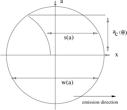
Figure 10: Definitons used in the text to calculate the integral over the emitting surface. Top view.

It is useful to define the following quantities, related to the selected coordinate system (see fig. 10), which follow from elemental trigonometry.

$$\theta_{c} = \arctan\frac{2r}{d}$$ (67)

$$a_{c}(\theta) = \sqrt{r^{2}-d^{2}/4\tan^{2}\theta}$$ (68)

$$w(a) = 2\sqrt{r^{2}-a^{2}}$$ (69)

$$s(\theta) = d\tan\theta$$ (70)

The angle $\theta_{\rm c}$ is the critical emission angle, above which some contributions to the integral vanish. $a_{c}(\theta)$ is the critical impact parameter where the mathematical form of the slices changes (see fig. 11 for a sketch of this). Above $\theta=\theta_{c}{\rm c}$ this expression no longer makes any sense. $w(a)$ is the ’width’ of the system for an impact parameter $a$ and determines the integration limits for the variable $x$. Finally $s(\theta)$ is used to divide the slice integral in the two different regions called $I$ and $II$ in fig. 11. With these conventions the integral splits in

$$I_{\nu} = I_{I+II}+I_{III+IV}$$ (71)

$$= 2(\int_{0}^{a_{c}}S_{1}(\theta)da+\int_{a_{c}}^{r}S_{2}(\theta)da)$$ (72)

where $S_{i}$ are the two types of slices that are possible in the system (see fig. 11).

Figure 11: Possible configurations of the integral over $x$ as a function of the other parameters.

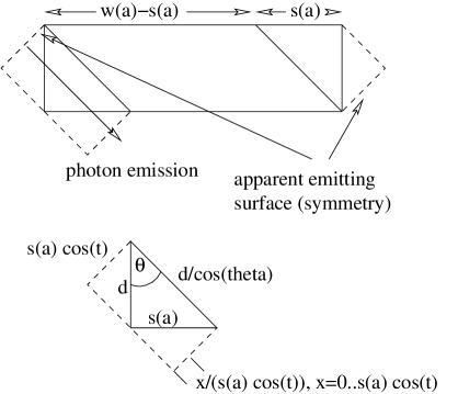
Figure 12: Detailed view of the geometry in the x-direction for small ’impact parameters’ $a$.

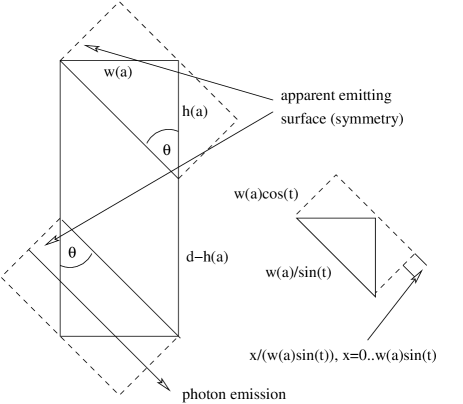
Figure 13: Detailed view of the geometry in the x-direction for large ’impact parameters’ $a$.

The first type of slice is the inner part of the disk (for small $a$), where some of the emitted photons (I) see a constant path length, where only the border region (II) is modified. Then the integral over $S_{1}$ can be solved exactly, and we get

$$S_{1} = (w(a)-s(\theta))\cos\theta(1-\exp(-\tau_{d}/\cos\theta))$$ (74)

$$+2\int_{0}^{s(\theta)\cos\theta}(1-\exp(\alpha\frac{d}{\cos\theta}\frac{x}{s(\theta)\cos\theta}))dx$$

$$= (1-\exp(-\tau_{d}/\cos\theta))\cdot$$

$$((w(a)-s(\theta))\cos\theta-2\frac{\sin\theta\cos\theta}{\alpha})$$

$$+2s(\theta)\cos\theta.$$

To solve the integral over $x$ we have used the parameterization $\tau(x)=\tau_{\rm max}\cdot x/x_{\rm max}$, with $0\leq x\leq x_{\rm max}$ (see fig.12). Inserting this expression in 72 and integrating over $a$ gives us

$$I_{1} = 2(1-\exp(-\tau_{d}/\cos\theta))\cdot$$ (75)

$$(\cos\theta(a_{c}w(a_{c})/2+r^{2}\arcsin{a_{c}/r})-a_{c}d\sin\theta$$

$$-2\frac{a_{c}\sin\theta\cos\theta}{\alpha})$$

$$+4a_{c}d\sin\theta\equiv I_{I+II}$$

which is the exact solution of the radiation transport equation for the region defined by $a<a_{\rm c}$.

The second type of slice, $S_{2}$ contains expressions that can not be solved analytically. The general structure of the integrals involved here is very similar to the $S_{1}$ contributions,

$$S_{2} = 2\int_{0}^{w(a)\cos\theta}(1-\exp(-\alpha\frac{w(a)}{\sin\theta}\frac{x}{w(a)\cos\theta}))dx$$ (77)

$$+(d-h(a))\sin\theta(1-\exp(-\tau_{w(a)}/\sin\theta))$$

$$= 2w(a)\cos\theta$$

$$+(1-\exp(-\tau_{w(a)}/\sin\theta))\cdot$$

$$((d-h(a))\sin\theta-2\frac{\sin\theta\cos\theta}{\alpha}).$$

Inserting this in eq. 72 results in non-analytical integrals,

$$I_{2} = \cos\theta(2\arccos\frac{a_{c}}{r}-a_{c}w(a_{c}))$$

$$+2\sin\theta(r-a_{c})(d-\frac{2\cos\theta}{\alpha})$$

$$+2\cos\theta\int_{a_{c}}^{r}w(a)\exp(-\frac{\tau_{w(a)}}{\sin(\theta)})da)$$

$$-2\sin\theta(d-2\frac{\cos\theta}{\alpha})\int_{a_{c}}^{r}\exp(-\frac{\tau_{w(a)}}{\sin(\theta)})da\equiv I_{III+IV}$$

The remaining integrals are of the form $\int\exp(-\sqrt{1-a^{2}})f(a)da$, which can only be solved in very special cases, such as $f(a)=a$. However, these integrals can be evaluated numerically in a fast and reliable way with the use of simple quadrature formulae of low order (see, e.g. Press et al. (1986-2001)).

Finally, for $\theta>\theta_{\rm c}$ the entire contribution $I_{1}$ vanishes, since in this case all slices are of the type ’2’, where all photons emitted from the top surface will leave the system through the side. So the total photon intensity emitted by a plasma in the form of a thin disk is

$$I(\theta<\theta_{c}) = I_{1}(a_{c}(\theta))+I_{2}(a_{c}(\theta))$$ (79)

$$I(\theta>\theta_{c}) = I_{2}(a_{c}=0).$$ (80)

Appendix B Solving the radiation transport equation with the exact square box geometry

The exact solution of the radiation transport equation takes a much simpler expression if one uses a box geometry. In fact, for this geometry all integrals are of the same type as the region called ’1’ in the last appendix, which does not involve any kind of numerical integrations. To keep the volume of the system constant, we use $a=\sqrt{\pi}r$ for the quadratic top and bottom surfaces and get

$$I_{box}(\theta<\theta_{c}) = a(1-\exp(\tau_{d}/\cos{\theta}))\cdot$$ (81)

$$(d\sin\theta-a\cos\theta-2\frac{\sin\theta\cos\theta}{\alpha})$$

$$+2ad\sin\theta$$

$$I_{box}(\theta>\theta_{c}) = a(1-\exp(\tau_{a}/\sin{\theta}))\cdot$$ (82)

$$(a\cos\theta-d\sin\theta-2\frac{\sin\theta\cos\theta}{\alpha})$$

$$+2a^{2}\cos\theta.$$

References

- Begelman et al. (1984) Begelman, M. C., Blandford, R. D., & Rees, M. J. 1984, Rev. Mod. Phys., 56, 255
- Butler & Buckingham (1962) Butler, S. & Buckingham, M. 1962, Phys. Rev., 126, 1
- Capella et al. (1994) Capella, A., Sukhatme, U., Tan, C.-I., & Tran, T. V. J. 1994, Phys. Rep, 236, 227
- Corbel et al. (2002) Corbel, S., Fender, R., Tzioumis, A., et al. 2002, Science, 298, 196