Dynamics of the Universe with global rotation

Abstract

We analyze dynamics of the FRW models with global rotation in terms of dynamical system methods. We reduce dynamics of these models to the FRW models with some fictitious fluid which scales like radiation matter. This fluid mimics dynamically effects of global rotation. The significance of the global rotation of the Universe for the resolution of the acceleration and horizon problems in cosmology is investigated. It is found that dynamics of the Universe can be reduced to the two-dimensional Hamiltonian dynamical system. Then the construction of the Hamiltonian allows for full classification of evolution paths. On the phase portraits we find the domains of cosmic acceleration for the globally rotating universe as well as the trajectories for which the horizon problem is solved. We show that the FRW models with global rotation are structurally stable. This proves that the universe acceleration is due to the global rotation. It is also shown how global rotation gives a natural explanation of the empirical relation between angular momentum for clusters and superclusters of galaxies. The relation $J\sim M^{2}$ is obtained as a consequence of self similarity invariance of the dynamics of the FRW model with global rotation. In derivation of this relation we use the Lie group of symmetry analysis of differential equation.

I Introduction

Rotation is a very universal phenomenon in nature. We can observe rotating objects at all scales of the Universe, from the elementary particles to planets, stars and galaxies. The question is, whether this property is an attribute of the whole universe at a very large scale structure. On the other hand, if our universe does not rotate, then the question is why and how does this happen? Since rotation is generic in the universe, the possible rotation of the universe cannot be excluded at the very beginning. Moreover, we should explain the physical mechanism which prevents universal rotation of the universe Obukhov02 .

Of course, if the Universe rotate, then there should exist some observational manifestations of this global rotation. Following the standard approach we can study the motion of test particles and photons on the background of corresponding spacetimes which admit the rotation. Our idea is to test the effects of rotation by classical cosmological tests like luminosity distance or angular size of radiogalaxies.

Since the work of Lanczos Lanczos24 , Gamov Gamov46 , Goedel Goedel49 , and Hawking Hawking69 , the cosmological models with rotation have been studied as well as the behavior of geodesics in such spacetimes. Although the quite strong upper limits for cosmic vorticity were obtained from analysis of CMB or BBN Hawking69 ; Collins73 ; Barrow85 ; Bunn96 ; Kogut97 all these works based on the model in which shear and vorticity effects are inseparable, i.e., in the sense that zero shear automatically implies zero vorticity. Therefore, the obtained limits actually placed not on the vorticity, but rather on the shear induced by it within the specific geometry of spacetime Obukhov02 . Finally, one thus needs a separate analysis of these limits in expanding cosmological models with trivial shear (shear-free) but non-zero rotation and expansion (it is an idea of Obukhov Obukhov02 ). Principally, there are two classes of such models in which this analysis can be performed

1. Newtonian shear-free models so-called Heckmann-Schücking models Heckmann59 ; Heckmann61 ;

2. general relativistic spatially homogeneous models with the geometry of the Bianchi IX and the cosmological constant Obukhov02 .

Let us consider the first class of models. We have a homogeneous Newtonian universe defined on product of the three-dimensional Euclidean space and absolute time coordinate. This universe is homogeneous, density and pressure of the fluid have no spatial dependence and the velocity vector field depends linearly on spatial coordinate Szekeres77 ; Senovilla98 . In this case contrary to the general relativity theory there exist shear-free solutions which satisfy the Heckmann-Schücking equations and describe both expanding and rotating universes Godlowski03 . The rotating homogeneous non-tilted universes when considered on a relativistic level filled with perfect fluid must have non-vanishing shear King73 ; Raychaudhuri79 . Therefore, it is very difficult to consider both effects of anisotropy and rotation, that’s why we study the Newtonian counterpart of model with rotation. Moreover, it is reasonable to assume that the shear scalar is sufficiently small compared with angular velocity scalar since the shear falls off more rapidly than the rotation as the universe expands Hawking69 ; Ellis73 ; Li98 ; Barrow04 .

To compare the results of analysis of supernovae data with a general relativistic model we formally consider a non-flat model $\Omega_{k,0}\neq 0$, although the satisfactory interpretation of $\Omega_{k,0}$ can be found beyond Newtonian cosmology in the general relativity.

The motion of the fluid in a homogeneous Newtonian universe is described by the scalar expansion $\theta$, the rotation tensor $\omega_{ab}$, and the shear tensor $\sigma_{ab}$. The homogeneous rotation of fluid as a whole is usually called the global rotation of the universe Li98 .

The problem of the rotation of the whole Universe attracted the attention of several scientists. It was shown, that the reported values are too big, when compared with the CMB anisotropy. Silk Silk70 pointed out that presently the dynamical effects of a general rotation of the Universe are unimportant, contrary to the the early universe, when angular velocity $\omega_{0}\geq 10^{-13}$ rad/yr. He stressed that now the period of rotation must be greater than the Hubble time, which is consequence of the CMB isotropy. Barrow Barrow85 also addressed this question and showed that the cosmic vorticity depends strongly on the cosmological models and assumptions connected with linearisation of homogeneous, anisotropic cosmological models over the isotropic Friedmann universe. For the flat universe they obtained the value ($\omega/H_{0})=2\cdot 10^{-5}$.

While the investigations of the cosmological models with global rotation has a long history, the global rotation of the Universe is still not detectable by observation. Some observational evidences for the global rotation of the Universe have not been confirmed Birch82 ; Phinney83 ; Bietenholz84 . The cosmological origin of the rotation of astronomical objects was analysed by Fil’chenkov in the framework of quantum cosmology and tunnelling approach Filchenkov03 .

The alignment of galaxies along the direction of the global rotation would also be some indication of the discussed phenomenon. However, the primordial dipole anisotropy of the distribution of rotation axes of galaxies is blurred due to the irregular shape of the protogalaxy, which can lead, after phase transition, to an almost random distribution. It is clear that the angular momentum of a structure is a sum of spins of components and its own angular momentum. A lot of work has been done in study of the alignment of galaxies in superclusters (for review see Djorgovski87 ). Here, the result are ambiguous, but several independent investigations claimed the existence of the weak alignment of galaxies in respect to the supercluster main plane Flin86 ; Kashikawa92 ; Godlowski93 ; Godlowski94 .

Independent observations of Supernovae type Ia (SNIa) have indicated that our Universe presently accelerates Perlmutter98 ; Perlmutter99 ; Garnavich98 ; Riess98 . There is a fundamental problem for theoretical physics to explain the origin of this acceleration. One of the first explanations was the cosmological constant. It is also possible to introduce the global rotation as we do in the present paper. While such a possibility seems to be attractive in the context of the accelerating universe, the cosmological constant is still needed to explain SNIa data because the contribution to acceleration coming from the global rotation is too small Godlowski03a .

In our previous papers we study some constraints on rotation coming from SNIa data, primordial nucleosynthesis as well as from the age of the oldest in the Universe Godlowski03a . The main aims of this paper is rather theoretical than empirical. We show that the analysis of the model dynamics is more effective after rewriting the basic equation to the new form with dimensionless quantities. Then we obtain a two-dimensional dynamical system in which coefficients have a simple interpretation of a density parameter of fluid fulfilling the Universe in the present epoch. In this approach dynamics is described by the Friedman-Robertson-Walker (FRW) model with some additional noninteracting fluid for which we can define density parameter $\Omega_{\omega}\equiv\rho_{\omega}/3H_{0}^{2}$. The presented formalism gives us also a natural base to discuss the influence of global rotation on acceleration of the Universe. From the observational constrains it is possible to find a limit for the angular velocity of the Universe. For example, Ciufolini and Wheeler Ciufolini95 obtained $\omega_{0}\simeq 6\cdot 10^{-21}\text{rad s}^{-1}\simeq 2\cdot 10^{-13}\text{rad yr}^{-1}$ from the CMB limit for the homogeneous B(IX) models with rotation. The limits for angular velocity of the Universe obtained from the CMB and SNIa were also discussed Godlowski03a . Here we also investigate some dynamical effects of the global rotation on the solving classical problems in cosmology, namely the horizon, flatness and cosmological constant problems.

Organization of our paper is as follows. In section 2 we present Hamiltonian dynamics of the FRW model with global rotation. In section 3 we discuss some properties of exact solutions with rotation. In section 4 we discuss the domains of the phase plane for which the cosmic acceleration and horizon problem are solved. In section 5 we construct the phase portraits for the FRW model with rotation and dust ($\gamma=1$). We also investigate general properties of dynamics by showing that generally it can be reduced to the form of the FRW models with non-interacting multifluid scaling like radiation. In section 6 a detailed analysis of dynamics on phase portrait is given in two dimensional phase plane. In section 7 we discuss the flatness and cosmological constant problems in the context of model with rotation. In section 8, it is proved (without of any help of empirical evidence) that formulae $J\sim M^{2}$ is exactly valid for the universe with dust ($\gamma=1$). For proof we use the Lie group theory of symmetry analysis of differential equations, describing the evolution of the universe. Then the relation between angular momentum and mass becomes a constraint relation between invariants of a self similarity group of symmetry of the basic equations. In section 9 we summarise obtained results.

II Reduced Hamiltonian Dynamics of FRW Universe with global rotation

In this paper we adopt the Hamiltonian formalism. It gives immediate insight into possible motion because the dynamical problem is analogous to that of a particle of unit mass moving in the one-dimension potential.

The Raychaudhuri equation describing the relation among scalar expansion $\Theta$, the rotation tensor $\omega_{ab}$ and shear tensor $\sigma_{ab}$ (if the acceleration vector $A^{a}\equiv u^{b}\nabla_{v}u^{a}$ vanishes, which would necessarily follow in the case of dust) has the form Ciufolini95

$$\dot{\Theta}=-\frac{1}{3}\Theta^{2}-2(\sigma^{2}-\omega^{2})+\Lambda-4\pi G(\rho+3p)$$ (1)

where $\omega^{2}=\omega_{ab}\omega^{ab}/2$, $\sigma^{2}=\sigma_{ab}\sigma^{ab}/2$, $\Lambda$ is the cosmological constant, $G$ is the gravitational constant, the fluid is perfect fluid with the stress-energy tensor $T_{ab}=(\rho+p)u_{a}u_{b}+pg_{ab}$ ($\rho$ is the mass density and $p$ is its pressure). The shear scalar $\sigma^{2}$ vanishes for the FRW model, while for the anisotropic Bianchi I or Bianchi V model (hereafter B(I) and B(V)) it satisfies the following equation

$$\frac{d\sigma^{2}}{dt}=-2\Theta\sigma^{2}.$$ (2)

Our aim is to consider the FRW model and its generalisation—anisotropic B(I) or B(V) models with global rotation. In the anisotropic generalization we have

$$3\Theta=(H_{1}+H_{2}+H_{3}),$$

where $H_{i}=d(\ln a_{i})/dt$ are the Hubble functions in three different main directions, and $a_{i}$ ($i=1,2,3$) are corresponding scale factors. Equation (1) can be also obtained within the Newtonian theory. However, in general relativity for the perfect fluid model with vanishing shear $\sigma=0$, and acceleration $\dot{u}_{a}=0$, the field equations can be consistent only if $\omega\Theta=0$. For the dust matter fluid with $\sigma=0$, $\dot{u}_{a}=0$, particles of dust are moving along geodesics. This is in contrast to the Newtonian case Ellis73 . Therefore, expanding and rotating spatially homogeneous universes filled with perfect fluid must have a non-interacting shear. Li Li98 considered the case that $\sigma$ is sufficiently small compared with $\omega$ since the shear following equation (2) falls off more rapidly than the rotation, during the expansion of the Universe Hawking69 . In the generic case in general relativity there is no solution with rotation and without shear. In other words, it has been shown that spatial homogeneous, rotating, and expanding universes with the perfect fluid have the nonvanishing shear Ellis73 ; Ciufolini95 . However, there exists such a possibility in the Newtonian cosmology because some standard obstacles of Newtonian cosmology can be overcome in this model Heckmann61 . The conservation of energy gives in a relativistic case

$$\dot{\rho}=-\Theta(\rho+p).$$ (3)

The occurrence of the term $p$ in the factor ($\rho+p$) has a special relativistic effect. It is a consequence of the inertia assigned to all forms of energy. The Newtonian counterpart of equation (3) corresponds to $p=0$ (dust for which world lines of fluid are geodesics Ellis73 ).

For a rotating, spherically symmetric, self-gravitating system with a characteristic size $R$, mean density $\rho$, and rotation $\omega$, the angular momentum $J$ is given by $J=2{\cal M}R^{2}\omega/5$. Therefore, the angular momentum conservation can be written in the Newtonian case in the form

$$\omega\rho a^{5}=\text{const}$$ (4)

where $a^{3}=a_{1}a_{2}a_{3}$ is an average scale factor. Principle (4) has its counterpart in the relativistic case Ellis73

$$\omega(\rho+p)a^{5}=\text{const}.$$ (5)

In the general relativistic case rotation is governed by a pair of nonlinear propagation and constraint equations which for the case of the barotropic equation of state reduces to Barrow04

$$\dot{\omega_{a}}=-\left[\frac{2}{3}\left(1-\frac{2}{3}c_{s}^{2}\right)\Theta-\sigma\right]\omega_{a}$$

where $\omega_{a}$ is a shear eigenvector ($\sigma_{ab}\omega^{2}=\sigma\omega_{a}$), and $c_{s}$ is a velocity of sound ($c^{2}_{s}=\frac{\partial p}{\partial\rho}$).

The Einstein equation for the considered case has a first integral in the form

$$\bar{H}^{2}=\frac{\Theta^{2}}{9}=\frac{8\pi G}{3}\rho-\frac{2}{3}\omega^{2}+\frac{\sigma^{2}}{3}-\frac{{}^{3}R}{6}+\frac{\Lambda}{3}$$ (6)

where ${}^{3}R$ is the Ricci scalar of three space equalled to $6k/a^{2}$ ($k=-1$ for B(V) and $k=0$ for B(I)) and for a natural system of units $8\pi G=c=1$. We usually work with the equation of state of the form

$$p=(\gamma-1)\rho$$ (7)

where $\gamma$ is a constant. From the physical point of view, the most important values are $\gamma=1$ (dust), $\gamma=4/3$ (radiation), $\gamma=2/3$ (strings), $\gamma_{\lambda}=2\gamma$ (brane effects), $\gamma=1/3$ (solid dark energy or topological defects). Let us note that in equation (6) there is no dependence on a particular form of the equation state.

If the matter is in a pressure-free form it is represented only by its 4-velocity $u^{a}$ and its energy density $\rho$. From the momentum conservation we obtain that matter moves along geodesics. For our further analysis it would be useful to rewrite equation (4) to the form of a differential equation

$$\dot{\omega}=-2\omega H\qquad\text{or}\qquad\dot{\omega}=(3\gamma-5)\omega H$$ (8)

for the equation of state in the form (7). After differentiation both sides of equation (6) with respect to the time variable and then the substitution of equation (6) we can obtain the Raychaudhuri equation. It explicitly demonstrates that in terms of the average Hubble function

$$\bar{H}=\frac{1}{3}(H_{1}+H_{2}+H_{3}),$$

equation (6) is really a first integral of basic equation (1). In the considered case we write this equation in the form

$$\dot{H}=-H^{2}-\frac{2}{3}(\sigma^{2}-\omega^{2})+\frac{\Lambda}{3}-\frac{1}{6}\rho(3\gamma-2),$$ (9)

where the bar over $H$ will be further omitted. For the FRW symmetry we have $H_{1}=H_{2}=H_{3}$, (but in general the Hubble function $H$ is understood to be averaged over three different main directions). For anisotropic models B(I) and B(V) the average Hubble parameter $\bar{H}$ is calculated from the average scale factor $\bar{H}=\ln(d/dt(\sqrt[3]{a_{1}a_{2}a_{3}}))$. Hence equation (9) for the model with the FRW symmetry can be rewritten to the form

$$\frac{\ddot{a}}{a}=-\frac{2}{3}(\sigma^{2}-\omega^{2})+\frac{\Lambda}{3}-\frac{1}{6}\rho(3\gamma-2)$$ (10)

where

$$\rho=\rho_{0}a^{-3\gamma},\qquad\sigma=\sigma_{0}a^{-3},\qquad\omega=\omega_{0}a^{-5+3\gamma}.$$

Let us note that from equation (8) we obtain that $\omega(a)$ does not preserve its form in different epochs. The value of $J$ depends on $\gamma$ ($J=\omega\rho\gamma a^{5}$). Of course

$$\frac{\dot{J}}{J}=\frac{\dot{\omega}}{\omega}+\frac{\dot{\rho}}{\rho}+5H=\frac{\dot{\omega}}{\omega}-3\gamma H+5H=0,$$

and conservation of $J$ takes place if only $\omega$ obeys relation (8).

Therefore the right-hand side of (10) can be expressed in terms of the scale factor $a$ (or average for B(I) and B(V))

$$\ddot{a}=\left(-\frac{2}{3}\sigma_{0}^{2}a^{-6}-\frac{3\gamma-2}{6}\rho_{0}a^{-3\gamma}+\frac{\Lambda}{3}+\frac{2}{3}\omega_{0}^{2}a^{-10+6\gamma}\right)a.$$ (11)

Equation (11) can be rewritten in the form analogous to the Newton equation of motion in the one-dimensional configuration space $\{a\colon a\in\mathbf{R}_{+}\}$ where $a$ is the scale factor

$$\ddot{a}=-\frac{\partial V}{\partial a}$$ (12)

where the potential function for $\gamma\neq 4/3$ is in the form

$$V(a)=-\frac{\sigma_{0}^{2}}{6}a^{-4}-\frac{\rho_{0}}{6}a^{-3\gamma+2}-\frac{\Lambda}{6}a^{2}-\frac{1}{3}\frac{\omega_{0}^{2}}{(3\gamma-4)}a^{2(3\gamma-4)}+V_{0}$$ (13)

while for $\gamma=4/3$ it takes the special form

$$V(a)=-\frac{\sigma_{0}^{2}}{6}a^{-4}-\frac{\rho_{0}}{6}a^{-2}-\frac{\Lambda}{6}a^{2}-C\ln a+V_{0}$$ (14)

where $V_{0}=\text{const}$ and $C$ is an undetermined integration constant in the Hamiltonian which the energy level should be consistent with the form of the first integral (6). Equation (12) has a first integral which can be expressed for $\gamma\neq 4/3$ in terms of the potential function $V(a)$ as

$$V(a)+\frac{\dot{a}^{2}}{2}=V_{0}-\frac{k}{2}.$$ (15)

Now we can construct the Hamiltonian

$$\mathcal{H}\equiv\frac{\dot{a}^{2}}{2}+V(a)$$ (16)

Trajectories of system (16) are situated on the distinguished energy level, $\mathcal{H}=E=\text{const}$. We can also define a new Hamiltonian flow in the one-dimensional configuration space on the zero energy level by translating the curvature contribution to the Hamiltonian. Then

$$\mathcal{H}=\frac{\dot{a}^{2}}{2}+V(a)=0$$ (17)

where for $\gamma\neq 4/3$

$$V(a)=-\frac{\sigma_{0}^{2}}{6}a^{-4}-\frac{\rho_{0}}{6}a^{-3\gamma+2}-\frac{\Lambda}{6}a^{2}-\frac{1}{3}\frac{\omega_{0}^{2}}{(3\gamma-4)}a^{2(3\gamma-4)}+\frac{k}{2}$$ (18)

and for $\gamma=4/3$ the Hamiltonian takes the special form

$$\mathcal{H}=\frac{\dot{a}^{2}}{2}+V(a)=-\frac{\sigma_{0}^{2}}{6}a^{-4}-\frac{\rho_{0}}{6}a^{-2}-\frac{\Lambda}{6}a^{2}-C\ln a+\frac{k}{2}+\frac{\dot{a}^{2}}{2}=E=-\frac{1}{3}\omega^{2}_{0}$$

which becomes consistent with the form of first integral (6) only for $C=0$. Therefore, for $\gamma\neq 4/3$ the physical trajectories lie on the zero-energy level $\mathcal{H}=E=0$ which coincide with the form of the first integral (18). For the special case of $\gamma=4/3$ trajectories lie on the distinguished energy level $\mathcal{H}=-\omega^{2}_{0}/3=\text{const}<0$. In both cases dynamics is given in the Hamiltonian form and trajectories lie on the distinguished level of constant energy. Finally, for radiation ($\gamma=4/3$) we obtain the new Hamiltonian considered on the zero energy level

$$\mathcal{H}=-\frac{\sigma_{0}^{2}}{6}a^{-4}-\frac{\rho_{0}}{6}a^{-2}+\frac{\dot{a}^{2}}{2}-\frac{\Lambda}{6}a^{2}+\left(\frac{k}{2}+\frac{1}{3}\omega_{0}^{2}\right)\equiv 0.$$ (19)

Note that this model is dynamically equivalent to standard model with some effective curvature,

$$k_{\text{eff}}=k+\frac{2}{3}\omega_{0}^{2}.$$ (20)

Let us consider the FRW ($\sigma_{0}=0$) model filled with some pure unknown matter $X$ such that $p_{X}=w_{X}\rho_{X}$. Then we obtain

$$V(a)=-\frac{\rho_{0}}{6}a^{-3w_{X}+2}+\frac{\Lambda}{6}a^{2}-\frac{\omega_{0}^{2}}{3(3w_{X}-4)}a^{2(3w_{X}-4)}+\frac{k}{2}.$$ (21)

The mixture of noninteracting dust and unknown matter $X$ satisfies the equation of state

$$p=p_{X}+0=(\gamma(a)-1)\rho=\frac{w_{X}}{\frac{\rho_{m0}}{\rho_{X0}}a^{3(w_{X}-1)}+1}\rho,\quad\rho=\rho_{m0}a^{-3}+\rho_{X0}a^{-3w_{X}}.$$ (22)

Then the potential function is given by the integral

$$V(a)=\int\limits^{a}\left[\frac{3(\gamma(a)-2)}{6}+\frac{2}{3}\sigma^{2}(a)-\frac{\Lambda}{3}-\frac{2}{3}\omega_{0}^{2}a^{-10}\exp\left(6\int\limits^{a}\frac{\gamma\left(a\right)}{a}da\right)\right]a\,da$$ (23)

where $\gamma(a)$ is derived from equation (22) and for the mixture of dust and unknown matter we can find that

$$\int\limits^{a}\frac{\gamma(a)}{a}da=\int\limits^{a}\frac{w_{X}\epsilon_{0x}a^{m-1}}{\epsilon_{0X}a^{m}+\epsilon_{0m}a^{-3}}da=\frac{w_{X}}{m+3}\ln(\epsilon_{0m}+\epsilon_{0X}a^{m+3})$$ (24)

where $m=-3(1+w_{X})$. Finally we obtain

$$V(a)=-\frac{\rho_{X0}}{6}a^{-3w_{X}+2}-\frac{\sigma_{0}^{2}}{6}a^{-4}-\frac{\Lambda}{6}a^{2}+\frac{k}{2}-\frac{2}{3}\omega_{0}^{2}\int\limits^{a}\frac{a^{-9}da}{(\epsilon_{0m}+\epsilon_{0X}a^{m+3})^{2}}$$ (25)

Let us consider for example the case of solid dark energy ($w_{X}=1/3$, $m=-4$). To do this we substitute these values into integral (24) which gives

$$\tilde{J}=\int\limits^{a}\frac{da}{a^{8}(\epsilon_{0m}+\epsilon_{0X})^{2}}=-\frac{1}{\epsilon_{0m}\epsilon_{0X}}\left[\frac{1}{a^{8}(1+\alpha a)}+8\sum\limits_{k=1}^{6}\frac{(-1)^{k}\alpha^{k-1}}{(7-k)!a^{7-k}}-\alpha^{6}\ln\frac{1+\alpha a}{a}\right]$$

where $\alpha={\epsilon_{0m}/\epsilon_{0X}}$.

Then we obtain potential in term of the integral $\tilde{J}$

$$V(a)=-\frac{\rho_{X0}}{6}a-\frac{\sigma_{0}^{2}}{6}a^{-4}-\frac{\Lambda}{6}a^{2}+\frac{k}{2}-\frac{2}{3}\omega_{0}^{2}\tilde{J}.$$ (26)

III Exact solution with rotation

In the case of the dust matter, an exact solution with rotation seems to be especially interesting. It can be easily shown that it can be simply obtained if we note that the corresponding dynamical equation reduces exactly to the best known case of the FRW model with dust, radiation, and the cosmological constant.

In the case of vanishing shear and the cosmological constant $\Lambda=0$ an exact solution can be given in the simplest form. There are three possibilities of positive ($k=+1$), zero ($k=0$), and negative ($k=-1$) curvature.

a) If $k=+1$ equation (17) becomes

$$\dot{a}^{2}=-2V(a)=\frac{\rho_{0}}{3}\frac{1}{a^{3\gamma-2}}+\frac{2}{3}\frac{\omega_{0}^{2}}{(3\gamma-4)a^{-6\gamma+8}}-1,$$

and since $\dot{a}^{2}$ has to be positive there are maximum and minimum values for $a$ (if $\gamma<4/3$) as can be derived using elementary techniques. The general solution for $\gamma=1$ (dust) is

$$t=-(\beta+\alpha a-a^{2})^{1/2}-\frac{\alpha}{2}\arcsin{\frac{\alpha-2a(t)}{(\alpha^{2}+4\beta)^{1/2}}}+C,$$

where $\alpha=\rho_{0}/3$, $\beta=-\frac{2}{3}\omega_{0}^{2}$ and $a_{\text{min}}<a<a_{\text{max}}=\frac{1}{2}((\alpha^{2}+4\beta)^{1/2}+\alpha)$, $\omega_{0}\leq\rho_{0}\sqrt{2}$.

Since only the first derivative vanishes for $a=a_{\text{max}}$, we obtain an oscillating singularity-free universe.

b) If $k=0$ equation (17) gives

$$\dot{a}^{2}=\frac{\alpha}{a^{3\gamma-2}}+\frac{\beta}{a^{-6\gamma+8}}.$$

Here $\dot{a}^{2}$ is always positive for $a>-\beta/\alpha$. So there is no maximum value for $a$. The result is a monotonically expanding universe without an initial singularity.

For $\gamma$=1 the general solution is

$$t=\frac{2}{3\alpha^{2}}(\alpha a+\beta)^{1/2}(\alpha a-2\beta)+C.$$

c) The last case, $k=-1$, gives the equation

$$\dot{a}^{2}=\frac{\alpha}{a^{3\gamma-2}}+\frac{\beta}{a^{-6\gamma+8}}+1.$$

This results is also a monotonically expanding universe without an initial singularity.

The scale factor has a minimum

$$a\geq a_{\text{min}}=\frac{-\alpha+\sqrt{\alpha^{2}-4\beta}}{2}.$$

For $\gamma=1$ the solution of (17) is

$$t=(a^{2}+\alpha a+\beta)^{1/2}-\frac{\alpha}{2}\ln{(2(a^{2}+\alpha a+\beta)+2a+\alpha)}+C,$$

if $\alpha^{2}-4\beta>0$,

$$t=(a^{2}+\alpha a+\beta)^{1/2}-\frac{\alpha}{2}\ln{(2a+\alpha)}+C,$$

if $\alpha^{2}-4\beta=0$,

$$t=(a^{2}+\alpha a+\beta)^{1/2}-\frac{\alpha}{2}\ln{(2a+\alpha)}+C.$$

Exact formulas for observables are also possible. For example, in the case of $\Lambda=0$ the luminosity distance $D_{0}$ between a galaxy, which emitted light at the cosmic moment $t$ and the observer who detected the light at the present moment $t_{0}$, is given by

$$D_{0}=\frac{\Omega_{\text{m},0}z+\left(\Omega_{\text{m},0}+2\Omega_{\omega,0}-1\right)\{[2\Omega_{\omega,0}z^{2}+2z\left(2\Omega_{\omega,0}+\Omega_{\text{m},0}\right)+1]^{1/2}-1\}}{H_{0}[\Omega_{\text{m},0}^{2}+2\Omega_{\omega,0}\left(2\Omega_{\omega,0}+2\Omega_{\text{m},0}-1\right)]}.$$

The above formula is valid for all values of curvature index (see for details Dabrowski86 ).

In the more general case of the nonvanishing cosmological constant we can find also a solution in the term of an elliptic function. In the case of dust matter, the problem of finding an exact solution is equivalent to integration of the equation

$$\left(\frac{dx}{dt}\right)^{2}=\Omega_{k,0}+\Omega_{\text{m},0}x^{-1}+\Omega_{\omega,0}x^{-2}+\Omega_{\Lambda,0}x^{2},$$

which takes the following form in the conformal time

$$\left(\frac{dx}{d\eta}\right)^{2}=\Omega_{\omega,0}+\Omega_{\text{m},0}x+\Omega_{k,0}x^{2}+\Omega_{\Lambda,0}x^{4}\equiv W(x),$$

where $d\eta\equiv dt/x$, $x\equiv a/a_{0}$ and $a_{0}$ is a present value of the scalar factor $a$.

Then it can be integrated explicitly using the Weierstrass $\wp$ function, to yield

$$\wp(\eta)=\frac{\sqrt{W(x)W(x_{0})}+W(x_{0})}{2(x-x_{0})^{2}}+\frac{4lx_{0}^{3}+2kx_{0}+m}{4(x-x_{0})}+\frac{6lx_{0}^{2}+k}{12}$$

or equivalently

$$x-x_{0}=\frac{\sqrt{W(x_{0})}\wp^{\prime}(\eta)+\frac{1}{2}[\wp(\eta)-\frac{6\Omega_{\Lambda,0}x_{0}^{2}+\Omega_{k,0}}{12}](4\Omega_{\Lambda,0}x_{0}^{3}+2\Omega_{k,0}x_{0}+\Omega_{m,0})+W(x_{0})\Omega_{\Lambda,0}x_{0}}{2[\wp(\eta)-\frac{6\Omega_{\Lambda,0}x_{0}^{2}+\Omega_{k,0}}{12}]^{2}-\frac{1}{2}\Omega_{\Lambda,0}W(x_{0})}$$

where $x_{0}=x(\eta=0)$, and $\wp$ is constructed with the invariants $g_{2}=\Omega_{\Lambda,0}\Omega_{\omega,0}+\frac{1}{12}\Omega_{k,0}^{2}$, $g_{3}=\frac{1}{6}\Omega_{\Lambda,0}\Omega_{k,0}\Omega_{\omega,0}-(\Omega_{k,0}/6)^{3}-\frac{1}{16}\Omega_{\Lambda,0}\Omega_{\text{m},0}$.

In the considered case the effect of the global rotation is modelled by negative radiation. Then, if we put in the place of dimensionless $\Omega_{r,0}$ some effective constant $\Omega_{\omega,0}^{\text{eff}}$, (which combine all contribution coming from matter scaling like radiation) we immediately obtain the exact solution in terms of the Weierstrass elliptic function Dabrowski86 . It is interesting that in this case formulas determining the magnitude-redshift relation can be also given in the exact form. After introducing $k_{\text{eff}}$ (see formula (20)) we can also simply obtain the corresponding exact formulas from that obtained for $\Omega_{k,0}\neq 0$.

IV Cosmic acceleration and horizon in the Universe with global rotation

In our further analysis we will explore dynamics given by the canonical equations. Assuming $x=a$ and $y=\dot{a}=\dot{x}$ we have from equation (17)

$$\dot{x} =\frac{\partial\mathcal{H}}{\partial y}=y$$ (27a)

$$\dot{y} =-\frac{\partial\mathcal{H}}{\partial x}=-\frac{\partial V}{\partial x}.$$ (27b)

with the first integral in the form $y^{2}/2+V(x)\equiv 0$. Then, we can perform a qualitative analysis of autonomous system (27) in the phase plane $(a,\dot{a})=(x,y)$.

The general observation is that if we consider the two-dimensional Hamiltonian dynamical system then eigenvalues of the linearization matrix $\lambda_{1},\lambda_{2}\colon\lambda^{2}=-\frac{\partial^{2}V}{\partial a^{2}}|_{a_{0}}$. They are saddle points if $\frac{\partial^{2}V}{\partial a^{2}}|_{a_{0}}<0$ and then eigenvalues are real of opposite signs otherwise they are centres at which eigenvalues are purely imaginary and conjugated. This dynamical system rewritten to more useful form will be considered in section 5.

We can also observe that trajectories of system (27) can be integrable in quadratures, namely, from the Hamiltonian constraint $\mathcal{H}=E=0$, we obtain

$$t-t_{0}=\int\limits_{a}\frac{da}{\sqrt{-2V(a)}}.$$ (28)

Note that it is possible to make the classification of qualitative evolution paths by analyzing the characteristic curve which represents the boundary of domain admissible for motion. For this purpose we consider the equation of zero velocity, $\dot{a}=0$ which represents the boundary in the configuration space. Because

$$\dot{a}^{2}=2V(a)$$ (29)

the motion of the system is limited to the region $\{a\colon V(a)\leq 0\}$. Let us consider the boundary set of the admissible for motion configuration space given by a condition

$$\partial M\equiv\{a\in\mathbf{R}_{+}\colon V(a)=0\}.$$ (30)

For the special case of $\gamma=4/3$ of course levels $V(a)=E$ should be considered. From the exact form of the potential function (18) or (23) parameters $\Lambda$ or $\omega_{0}$ can be expressed as a function of $a$. For example from (18) for $\gamma\neq 4/3$ we obtain

$$\Lambda(a)=\frac{6}{a^{2}}\left[-\frac{\sigma_{0}^{2}}{6}a^{-4}-\frac{\rho_{0}}{6}a^{-3\gamma+2}-\frac{1}{3}\frac{\omega_{0}^{2}}{(3\gamma-4)}a^{2(3\gamma-4)}+\frac{k}{2}\right]$$ (31)

and for $\gamma=4/3$

$$\Lambda(a)=\frac{6}{a^{2}}\left[-\frac{\sigma_{0}^{2}}{6}a^{-4}-\frac{\rho_{0}}{6}a^{-2}-\frac{2}{3}\omega_{0}^{2}+\frac{k}{2}\right].$$ (32)

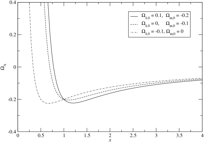
Figure 2: Diagram of the $\Omega_{\Lambda}(x)$ density parameter given by relation: $\Omega_{\Lambda}(x)=-\frac{\Omega_{k,0}x^{2}+\Omega_{\text{m},0}x^{3}+\Omega_{\omega,0}}{x^{4}}$ for different values of ($\Omega_{k,0}$, $\Omega_{\text{m},0}$, $\Omega_{\omega,0}$). Forbidden (non physical) region: $y^{2}/2<0$ is situated under the characteristic curve. The lines $\Omega_{\Lambda}(a)=\text{const}$ gives qualitative classification of possible path evolutions in the configuration space. The minimum is reached for $\Omega_{k,0}=0$ at $x_{\text{min}}=\sqrt[3]{\frac{-4\Omega_{\omega,0}}{\Omega_{\text{m},0}}}=\sqrt[3]{\frac{16\omega_{0}^{2}}{3\Omega_{\text{m},0}}}$. Note the existence of oscillating models without the singularity for $\Omega_{\Lambda,0}<0$.

Finally, we consider the evolution path as a level of $\Lambda=\text{const}$ and then we classify all evolution scenarios modulo with their quantitative properties of dynamics (to compare see Robertson33 ; Dabrowski96 ). For the special case of radiation the corresponding classification of the FRW model effective curvature $k_{\text{eff}}$ can be achieved in a similar way. Then we obtain the analogous phase portraits is shown on Fig. 2.

From the physical point of view it is interesting to answer the questions: are the trajectories distributed in the phase space in such a way that critical points are typical or exceptional? How are trajectories with interesting properties distributed? For example, along which trajectories the acceleration condition, $\ddot{a}=-dV/da>0$ is satisfied? In order to fulfil that $V(a)$ must be decreasing. One can easily observe this phenomenon from the geometry of the potential function. In the phase space, the area of accelerations is determined by condition $\dot{y}>0$ or by corresponding condition in the configuration space

$$\frac{2}{3}\sigma_{0}^{2}a^{-6}+\frac{3\gamma-2}{6}\rho_{0}a^{-3\gamma}-\frac{\Lambda}{3}-\frac{2}{3}\omega_{0}^{2}a^{-10+6\gamma}<0.$$ (33)

The presence of the last term in inequality (33) demonstrates that in the configuration space the domain of acceleration is larger than for the case of the FRW model with vanishing global rotation. Let us note that the positive value of the cosmological constant $\Lambda$ acts in the same direction as rotation, i.e., global rotation acts as dark energy (or dark radiation).

It can easily be demonstrated for the FRW models that if $\dot{a}(t)\to\text{const}$ as $a\to 0$ then the model has no particle horizons (in the past) Weinberg72 . Indeed, if there exists a constant $C$ such as for sufficiently large $\rho$, the velocity of the scale factor is upper bounded $da/dt\leq C$ and

$$\int\limits_{0}^{a_{0}}\frac{da}{a}<C\int\limits_{0}^{t_{0}}\frac{dt}{a}.$$ (34)

The integral on the left hand-side of (34) diverges and there are no causally disconnected regions. Putting this in terms of $(x,y)$ variables one needs the condition, as $x\to 0$, $y\to\text{const}$, as the sufficient condition for solving the horizon problem. Now, from the Hamiltonian constraint we obtain that as $x\to 0$, then $V(x)\to\text{const}$ (zero is included).

V The phase plane analysis—general properties of the models

Let us apply a dynamical system method to analyse the system under consideration. The dynamics of cosmological models with global rotation, the cosmological constant $\Lambda$ and matter, satisfying the equation of state (7), is described by the following dynamical system

$$\dot{a} =y$$ (35a)

$$\dot{y} =-\frac{2}{3}\sigma_{0}^{2}a^{-5}-\frac{3\gamma-2}{6}\rho_{0}a^{-3\gamma+1}+\frac{\Lambda}{3}a+\frac{2}{3}\omega_{0}^{2}a^{6\gamma-9}.$$ (35b)

Let us note that some general properties of system (35) for vanishing shear ($\sigma_{0}=0$) and the matter in the form of solid dark energy (or topological defects) with $\gamma=1/3$. Then when $a\to 0$ the effect of the cosmological constant is negligible. In this case $\dot{y}=\frac{1}{6}\rho_{0}+\frac{2}{3}\omega_{0}^{2}a^{-7}$ and the term with rotation cannot dominate the matter term with positive energy because $V(a)\leq 0$. From the existence of the first integral we have

$$y=\sqrt{-2V(a)}=\sqrt{\frac{1}{3}\rho_{0}a+\frac{2}{3}\omega_{0}^{2}a^{-5}-k}\qquad\text{and}\qquad a>\left(\frac{2}{3\rho_{0}}\omega^{2}_{0}\right)^{1/7}.$$

It is possible that density of solid dark energy and the rotation compensate each other, when the scale factor reaches $a=a_{\text{min}}$ near the singularity.

As $a\to 0$ we have $\dot{y}=\frac{1}{6}\rho_{0}$, i.e., $y\sim t$ and $a\sim t^{2}$ and we obtain that the horizon problem is solved because $y=\dot{a}\to 0$ as $t\to 0$. The phase portrait for this case show Fig. 1.

To apply the method of dynamical system let us consider the FRW model with dust matter, the cosmological constant, and global rotation. Then the corresponding dynamical system has the form

$$\dot{a} =y$$ (36a)

$$\dot{y} =-\frac{1}{6}\rho_{0}a^{-2}+\frac{\Lambda}{3}a+\frac{2}{3}\omega_{0}^{2}a^{-3}$$ (36b)

with the first integral, for the general form of the equation of state $p=(\gamma-1)\rho$, given by

$$y^{2}=\frac{1}{3}\rho_{0}a^{-1}+\frac{\Lambda}{3}a^{2}-k-\frac{2}{3}\omega_{0}^{2}\frac{a^{2(3\gamma-4)}}{3\gamma-4},$$ (37)

Near the initial singularity of type, i.e., as $a\to\text{const}$ the generic flat solution without the cosmological constant has the form

$$t-t_{0}=\frac{2}{3\rho^{2}_{0}}\left(\frac{\rho_{0}}{3}a+\frac{4}{3}\omega^{2}_{0}\right)\sqrt{\frac{\rho_{0}}{3}a+\frac{2}{3}\omega^{2}_{0}}.$$ (38)

If we assume that $\omega_{0}\ll 1$ then from solution (38) we obtain a simple monotonic solution with the singularity at $a=a_{0}=\frac{2\omega^{2}_{0}}{\rho_{0}}$

$$t-t_{0}=\frac{2a}{9\sqrt{3\rho^{2}_{0}}}\sqrt{a+\frac{2\omega^{2}_{0}}{\rho_{0}}}.$$ (39)

Note, that as in the previous case there is the possibility that the scale factor reaches $a=a_{\text{min}}$ in the initial singularity. From the condition that motion is admissible in the region $V(x)\leq 0$ we have for the flat model the condition

$$\forall x\colon-\frac{1}{2}\Omega_{\text{m},0}x^{-1}-\frac{1}{2}\Omega_{\omega,0}x^{-2}<0$$

or in terms of redshift $z$

$$\forall z\colon\Omega_{\text{m},0}+\Omega_{\omega,0}(1+z)>0.$$

For the minimum $a=a_{\text{min}}$ and the maximum $\rho_{\text{m}}$ we finally obtain the bound

$$-\Omega_{\omega,0}<\frac{\Omega_{\text{m},0}}{1+z_{\text{sing}}},$$

where $\Omega_{\text{m},0}\simeq 0.3$ and $z_{\text{sing}}$ is the value of redshift at the moment of singularity $a=a_{\text{min}}$ such that $1+z_{\text{sing}}=\frac{a_{0}}{a_{\text{min}}}$. It would be useful to compare the present effects of radiation and rotation because both scale in the same way. The rotation effect could dynamically dominate radiation i.e.,

$$-\Omega_{\omega,0}>\Omega_{r,0}\simeq 0.5\cdot 10^{-4}.$$

The contribution coming from both radiation and rotation we denote as $\Omega^{\text{total}}_{r,0}$. Then, from equation (36b) in the case without the cosmological constant it can be obtained the relation

$$\ddot{x}=-\frac{\Omega_{\text{m},0}}{2}x^{-2}\left(1+\frac{2\Omega^{\text{total}}_{r,0}}{\Omega_{\text{m},0}}x^{-1}\right).$$

Therefore, for $x_{0}=-\frac{2\Omega^{\text{total}}_{r,0}}{\Omega_{\text{m},0}}$ we have an inflection point on diagram $x(t)=\frac{a}{a_{0}}$ which separates domains in which $\ddot{x}$ has different convexity.

Our starting point for further analysis of results will be dynamical equations rewritten to the new form using dimensionless quantities:

$$x\equiv\frac{a}{a_{0}},\qquad T\equiv|H_{0}|t,\qquad\Omega_{i,0}\equiv\frac{\rho_{i,0}}{\rho_{\text{cr},0}},$$ (40)

$$\rho=\rho_{0}\left(\frac{a}{a_{0}}\right)^{-3\gamma},\qquad\sigma=\sigma_{0}\left(\frac{a}{a_{0}}\right)^{-3},\qquad\omega=\omega_{0}\left(\frac{a}{a_{0}}\right)^{-5+3\gamma},$$ (41)

with $H=\frac{\dot{a}}{a}$, $\rho_{\text{cr}}=3{H_{0}}^{2}$ where the index $0$ denotes present day values (at time $t_{0}$). After introducing the density parameter of rotation for $\gamma\neq 4/3$ the dynamical effect of global rotation is equivalent to some kind of additional, noninteracting fluid for which we have

$$\rho_{\omega}=\frac{2\omega_{0}^{2}}{3\gamma-4}x^{2(3\gamma-5)}=\rho_{\omega_{0}}x^{6\gamma-10},\qquad\Omega_{\omega}=\frac{\rho_{\omega}}{\rho_{cr}}=\Omega_{\omega,0}x^{6\gamma-10},$$ (42)

$$w_{\omega}=\frac{10-6\gamma}{3},\qquad p_{\omega}=(w_{\omega}-1)\rho_{\omega},$$ (43)

and negative energy and in consequence the negative density parameter $\Omega_{\omega}$. Hence, the basic dynamical equations are

$$\frac{\dot{x}^{2}}{2}=\frac{1}{2}\Omega_{k,0}+\frac{1}{2}\sum\limits_{i=1}\Omega_{i,0}x^{2-3w_{i}}\\$$ (44)

$$\dot{x} =x$$ (45a)

$$\dot{y} =\ddot{x}=\frac{1}{2}\sum\limits_{i=1}\Omega_{i,0}(2-3w_{i})x^{1-3w_{i}}=-\frac{\partial V}{\partial x}.$$ (45b)

where for $w_{i}\neq 2/3$ ($\gamma\neq 4/3$)

$$V(x)=-\frac{1}{2}\Omega_{k,0}-\frac{1}{2}\sum\limits_{i=1}{\Omega_{i,0}x^{2-3w_{i}}},$$ (46)

$$\frac{1}{2}\Omega_{\omega,0}=\frac{2}{3}\frac{\omega_{0}^{2}}{(3\gamma-4)},$$

and the system is now defined on the zero energy level $\mathcal{H}=E=0$.

If $w_{i}=2/3$ ($\gamma=4/3$) we have

$$V(x)=\frac{1}{2}\sum\limits_{w_{i}\neq 1}{\Omega_{i,0}x^{2-3w_{i}}}+\frac{1}{3}\omega^{2}_{0},$$ (47)

where in general $p_{X}=(w_{X}-1)\rho_{X}$ and for unknown dark energy $X$, $w_{1}=1/3$ (solid dark energy), $w_{2}=2/3$ (effects of string), $w_{3}=\gamma$ (perfect fluid), $w_{\Lambda}=0$ (cosmological constant), $w_{\omega}=\frac{10-6\gamma}{3}$ (for rotation), $w_{\lambda}=2\gamma$ (effects of brane).

We could in principle include the curvature term $\frac{1}{2}\Omega_{k,0}$ into the sum in the right hand sides of (44), it would correspond to $w_{k}=2/3$. We see that in particular the case $x_{0}=1$, $\dot{x}_{0}=1$ is a solution. From this definition $\ddot{x}_{0}=-q_{0}$, where $q_{0}$ is the deceleration parameter. Therefore, $\sum\limits\Omega_{i,0}+\Omega_{k,0}=1$ (presently but this equality can be extended to any given time). For the special case of the universe filled with radiation matter we can also formally define energy density of some fictitious fluid which mimics the rotation effect and scales like “curvature fluid”, $\rho_{\omega}=-2\omega^{2}_{0}a^{-2}$. Hence, the corresponding density parameter is

$$\Omega_{\omega}=\frac{\rho_{\omega}}{3H_{0}^{2}},\qquad$$

and because the system is defined on the levels $\mathcal{H}=E=0$ we have the constraint $\sum_{i}\Omega_{i,0}=1$.

Therefore in any case the system under consideration can be represented in the form of the multifluid FRW dynamics. Of course, dynamical system (45) is the Hamiltonian

$$\mathcal{H}=\frac{p_{x}^{2}}{2}+V(x)$$ (48)

where $p_{x}$ is the momentum conjugated with the generalised coordinate $x$.

In the following we consider a universe filled with dust and some unknown component $X$ with negative pressure called “dark energy”, so that the strong energy condition is violated $\rho_{X}+3p_{X}<0$. We assume that the weak energy condition $\rho_{X}+p_{X}>0$ is satisfied, so $w_{X}>0$ for the hypothetical quintessence matter. Hence, the Universe is accelerating provided that the following condition is satisfied

$$2\ddot{a}(x)=\Omega_{X,0}(2-3w_{X})x^{1-3w_{X}}-\Omega_{\text{m},0}x^{-2}+2\Omega_{\omega,0}(3\delta(x)-4)x^{3(2\gamma-3)}+2\Omega_{\Lambda,0}x>0,$$ (49)

where

$$\delta(x)=\frac{w_{X}}{\frac{\Omega_{\text{m},0}}{\Omega_{X,0}}x^{3(w_{X}-1)}+1},\qquad p=\delta(x)\rho$$

and $p,\rho$ are total pressure and energy density; $p=0+w_{X}\rho_{X}$, $\rho=\rho_{m}+\rho_{X}$.

Our universe accelerates at present ($x=1$) if

$$\Omega_{X,0}(2-3w_{X})-\Omega_{\text{m},0}+2\Omega_{\omega,0}(3\delta(1)-4)+2\Omega_{\Lambda,0}>0.$$ (50)

Let put $\Omega_{\Lambda,0}=0$ and matter $X$ denotes a candidate for the dark energy (the pure cosmological constant corresponds to $w_{X}=-1$).

Let $\sigma=\Omega_{\text{m},0}/\Omega_{X,0}$, $\delta=\Omega_{\omega,0}/\Omega_{X,0}$, then is required

$$w_{X}<\frac{(8\delta+\sigma-2)(\sigma+1)}{3(2\delta-\sigma-1)}.$$ (51)

If $\sigma=3/7$ then for small $\delta$ we have

$$w_{X}\leq\frac{11}{21}(1+40.6|\delta|),\qquad\delta<0.$$ (52)

Therefore, the corresponding conditions of negativeness of coefficient of state for dark energy is weaker then for the case of vanishing rotation. Present experimental estimates are based on estimation of barions in clusters of galaxies giving $\Omega_{\text{m},0}\sim 0.3$ Peebles03 . On the other hand, the location of the first acoustic peak in the CMB detected by the experiments Boomerang, Maxima and WMAP suggest a nearly flat universe. It also implies that our Universe is presently accelerating for a wide range of values of coefficients of the equation of state, roughly $w_{X}<0.5$. Let us note that now we have the constraint on the angular velocity

$$\omega_{0}=\sqrt{\frac{3\left(\Omega_{k,0}+\Omega_{\text{m},0}+\Omega_{\Lambda,0}-1\right)}{2}}H_{0}=\sqrt{\frac{-3\Omega_{\omega,0}}{2}}H_{0}$$ (53)

which is obtained as a consequence of the constraint relation $\Sigma\Omega_{i,0}=1$.

It is easy to obtain that for $\Omega_{\omega,0}\sim 0.01$ which corresponds to the limit obtained by us from SNIa data and the present value $\rho_{0}=0.8\cdot 10^{-29}$ g cm^-3, $\omega_{0}\sim 2.6\cdot 10^{-19}$ rad s^-1 that is in a good agreement with the observational limit Godlowski04 .

Let us now make some important remarks concerning acceleration regions transition in the configuration space admissible for motion $x_{\text{min}}<x\leq\infty$. The “physical region” is $x_{\text{min}}<x\leq 1$ because $x\equiv a/a_{0}$. Accelerated expansion starts from same $x_{a}$ given by non-zero solutions of the equation

$$h(x)=-\frac{\partial V(x)}{\partial x}x^{3}=-\Omega_{\text{m},0}x+2\Omega_{\Lambda,0}x^{4}-2\Omega_{\omega,0}=0$$

which represents the boundary of acceleration region $h(x)\geq 0$ in the configuration space.

The function $h(x)$ satisfies the condition $h^{\prime\prime}(x)>0$ if only $\Omega_{\Lambda,0}>0$ and for large and small $x$ where it has asymptotic forms $h(x)\propto\Omega_{\Lambda,0}x^{4}$ and $h(x)=-\Omega_{\text{m},0}x-2\Omega_{\omega,0}$, respectively. Additionally, we have $h(0)=-2\Omega_{\omega,0}>0$. Therefore, $h(x)$ has a minimum at $x_{\text{min}}=\sqrt[3]{\Omega_{\text{m},0}/2\Omega_{\Lambda,0}}$ which coincides with the same value for the standard case with vanishing $\Omega_{\omega,0}$.

Let us consider the model without rotation $\Omega_{\omega,0}=0$. Then $x\in[0,1]$. Now, we can simply define the fraction of acceleration during the whole evolution up today as

$$P=\frac{1-x_{a}}{1}=1-\sqrt[3]{\frac{\Omega_{\text{m},0}}{2\Omega_{\Lambda,0}}},$$

where $x_{a}=\frac{a_{\text{tr}}}{a_{0}}$ is the value of the relative scale factor in the transition epoch $a_{\text{tr}}$. For these models accelerated expansion starts at $x_{a}$, which corresponds to transition redshift

$$z_{a}=x_{a}^{-1}-1=\sqrt[3]{\frac{2\Omega_{\Lambda,0}}{\Omega_{\text{m},0}}}-1.$$

The fact that $z_{a}$ is so close to zero (for the FRW model with the cosmological constant term, $z_{a}=0.414$) is the cosmic coincidence problem—$z_{a}$ is shifted towards smaller redshift.

Let us note that this obstacle is less dramatic in the class of models with rotation $\Omega_{\omega,0}\neq 0$, because due to presence of rotation contribution $z_{a}$ is shifted towards larger redshift.

VI Discussion and detailed analysis of the phase plane

Dynamical system methods of analysis dynamics of the FRW model with global rotation seems to be useful if we are interested in the qualitative properties of dynamics and influence of global rotation on the dynamics of the universe. In this approach we deal with the full global dynamics of the universe whose asymptotic states are represented by critical points of the systems. In such a representation the phase diagrams in a two-dimensional phase space allow us to analyse the acceleration in a clear and natural way. It is the consequence of representation of dynamics as a one-dimensional Hamiltonian flow.

From the theoretical point view it is important to know how large the class of accelerated models is, or what kind of qualitative behaviour of trajectories introduce the global rotation. We will call this class of accelerated models typical (or generic), if the domain of acceleration in the phase space driven by effect of global rotation is non-zero measure. On the other hand, if only nongeneric (or zero measure) trajectories are represented by accelerated universes, then the mechanism which drives these trajectories to accelerate should be called ineffective. Such a point of view is a consequence of the fact that, if the acceleration is an attribute of a trajectory which starts with a given initial condition it should also be an attribute of trajectories which start from nearby initial conditions. From recent astronomical measurements we obtain that while global rotation effects give rise to the acceleration of the universe, the cosmological constant is still needed to explain its rate.

The system under consideration is

$$\dot{x} =y$$ (54a)

$$\dot{y} =-\frac{1}{2}\sum_{i}\Omega_{i,0}(3w_{i}-2)x^{1-3w_{i}}=-\frac{\partial V}{\partial x}$$ (54b)

with first integral

$$\frac{y^{2}}{2}-\frac{1}{2}\sum_{i}\Omega_{i,0}x^{2-3w_{i}}=0.$$

In general, it represents the dynamics of FRW models filled with noninteracting multifluid for each $i$ component in the equation of state $p_{i}=(w_{i}-1)\rho_{i}$ is satisfied.

For the FRW model with global rotation, the cosmological constant and dust we have

$$w_{\omega}=\frac{10-6\gamma}{3},\qquad w_{k}=\frac{2}{3},\qquad\gamma=1$$

and

$$\dot{x} =y$$ (55a)

$$\dot{y} =-\frac{1}{2}\Omega_{\text{m},0}x^{-2}-\Omega_{\Lambda,0}x-\Omega_{\omega,0}x^{-3}$$ (55b)

System (55) has the first integral given by

$$y^{2}=-\frac{1}{2}\Omega_{\text{m},0}x^{-1}+\Omega_{k,0}+\Omega_{\Lambda,0}x^{2}+\Omega_{\omega,0}x^{-2}.$$ (56)

The classification of all admissible evolutional paths in the configuration space is demonstrated in Fig. 2. The phase portrait which visualizes the all evolutions for all initial conditions is presented on Fig. 3. For comparison the phase portrait with the cosmological constant, and topological defects is in Fig. 1. The concordance $\Lambda$CDM model is shown on Fig. 4.

The critical points of (55) are solutions of the equations

$$V(x_{0},y_{0})=0\Leftrightarrow\Omega_{\omega,0}x^{-2}+\Omega_{\text{m},0}x^{-1}+\Omega_{k,0}+\Omega_{\Lambda,0}x^{2}=0$$ (57)

and

$$\left.\frac{\partial V}{\partial x}\right|_{(x_{0},y_{0})}=0\Leftrightarrow-\Omega_{\omega,0}x^{-3}-\frac{1}{2}\Omega_{\text{m},0}x^{-2}+\Omega_{\Lambda,0}x=0$$ (58)

where $\sum_{i}\Omega_{i,0}=1$.

Trajectories of the system belong to the domain admissible for motion

$$\mathcal{D}=\{(x,y)\in\mathbf{R}^{2}\colon x_{\text{min}}<x\ \text{and}\ V(x)\leq 0\}.$$

Therefore, critical points lie on the boundary $\partial\mathcal{D}=\{x\colon V(x)=0\}$

$$V(x)=-\frac{1}{2}x^{-2}(\Omega_{\omega,0}+\Omega_{\text{m},0}x+\Omega_{k,0}x^{2}+\Omega_{\Lambda,0}x^{4}).$$

To find the solution $x_{0}$ of (57) and (58) we consider the probe equation which helps us to formulate necessary condition for $x_{0}\neq 0$ to be solution if only

$$-\Omega_{\omega,0}+\Omega_{k,0}x^{2}+3\Omega_{\Lambda,0}x^{4}=0.$$

Of course, if both $\Omega_{\Lambda,0}$ and $\Omega_{k,0}$ are positive then there is no critical point in the finite domain.

Let us consider the case of $\Omega_{k,0}<0$. Then

$$x_{0}=\sqrt{\frac{-\Omega_{k,0}-\sqrt{\Omega_{k,0}^{2}+12\Omega_{\omega,0}\Omega_{\Lambda,0}}}{6\Omega_{\Lambda,0}}},\qquad y_{0}=0.$$

where it is assumed that rotation is sufficiently small to ensure that real $x_{0}$ exists, i.e.,

$$-\Omega_{\omega,0}<\frac{\Omega_{k,0}^{2}}{12\Omega_{\Lambda,0}}.$$

In the opposite case if the contribution coming from rotation is sufficiently large, the domain admissible for motion is empty.

Finally, the smallest value of $x=x_{0}$ is given by $V(x_{0})=0$ because the critical points must be always a zero of the potential function.

From the physical point of view the critical point of this type represents the static Einstein universe.

Let us briefly comment now on the case of vanishing rotation in the above context. Then the domain admissible for motion is for positive $x$. In the phase space all critical points are situated at the $x$-axis, at the point

$$x_{0}=\sqrt{-\frac{\Omega_{k,0}}{3\Omega_{\Lambda,0}}},\qquad y_{0}=0.$$

Therefore, we have always static critical points if only $\Omega_{k,0}$ and $\Omega_{\Lambda,0}$ are of opposite signs.

The character of the critical point is determined from eigenvalues of the linearization matrix at critical point or equivalently from the convectivity of $V(x)$

$$\frac{\partial^{2}V}{\partial x^{2}}=-3\Omega_{\omega,0}x^{-4}-\Omega_{\text{m},0}x^{-3}-\Omega_{\Lambda,0}$$

but from (57) we have at the critical point

$$-\Omega_{\omega,0}x_{0}^{-4}=\frac{1}{2}\Omega_{\text{m},0}x_{0}^{-3}-\Omega_{\Lambda,0}.$$

Then for any $x_{0}$ we have

$$\left.\frac{\partial^{2}V}{\partial x^{2}}\right|_{(x_{0},0)} =-\frac{5}{2}\Omega_{\text{m},0}x_{0}^{-3}-4\Omega_{\Lambda,0}<0\qquad\text{or in general}$$

$$\left.\frac{\partial^{2}V}{\partial x^{2}}\right|_{(x_{0},0)} =\det A=-\lambda_{1}\lambda_{2}$$

where $\lambda_{i}$ $(i=1,2)$ are eigenvalues of the linearization matrix $A$ of the system

$$A=\left[\begin{array}[]{cc}0&1\\ -\frac{\partial^{2}V}{\partial x^{2}}&0\end{array}\right].$$

Then eigenvalues are solutions of the characteristic equation $\lambda^{2}-(\mathop{\text{tr}}A)\lambda+\det A=0$ for the matrix $A$.

Finally, we show that in the physical domain our system with positive curvature $k>0$ has at least one critical point which is represented on phase plane by the saddle point.

Let us consider the phase portrait of the system with global rotation and dust matter on the phase plane $(x,y)$. We assume the existence of the non-vanishing cosmological term because the value $\Omega_{\Lambda,0}\neq 0$ is required by consistency of the model with global rotations with SNIa data.

If we consider the standard FRW cosmology on the $(x,y)$ plane then situation is presented in Fig. 4. The flat model trajectory separates the region of the model with negative and positive curvature. The critical point is a saddle and it represents the static Einstein solution. Non-generic cases corresponding to separatices going in or out of the saddle point. The acceleration region is situated on the right from the saddle point. Therefore the recollapsing and then expanding models lie permanently in the acceleration domain and there is a transition from decelerating to accelerating epochs. The Eddington model is also in this region. The Lemaître-Eddington models start accelerating in the middle of the quasi static phase. As we can see from Fig. 1 the global rotation contribution introduces qualitative changes of behaviour of trajectories, i.e., there is no homeomorphism which preserves directions along trajectories and transforms the corresponding the trajectories. In our case there is no critical points on the phase plane at the finite domain (Fig. 1). It can be shown that in general if only $a>\left(\frac{3\rho_{0}}{4\Lambda}\right)^{1/3}=a_{\text{min}}$, then there is no critical point representing a static Einstein universe.

To analyse system (55) at infinity it is useful to introduce the projective map $(v,u)\colon v=1/x$, $u=y/x$ on the plane and

$$\dot{v} =-uv$$ (59a)

$$\dot{u} =-\frac{1}{2}\Omega_{\text{m},0}v^{3}-\Omega_{\omega,0}v^{4}+\Omega_{\Lambda,0}-u^{2}$$ (59b)

Then, circle at infinity is covered by line $v=0$ ($x=\infty$). The dynamical system with the non-zero cosmological constant and non-vanishing global rotation in the finite region is presented in Fig. 5. The region $x<x_{\text{min}}$ is forbidden because the global rotation contribution cannot dominate the matter contribution. In this case there is one type of trajectories which recollapses from the initial singularity and then expands after reaching the minimum size of scale factor. Hence the expanding de Sitter model is a global attractor and the contracting de Sitter one is a global repeller (Fig. 5). All point at infinity which lies on $v=0$ circle are hyperbolic, therefore the system is structurally stable.

Figure 1: The phase portrait of system for models with global rotation $\Omega_{\omega,0}\neq 0$ and dark matter $X$ in the form of solid dark energy ($w_{X}=1/3$), i.e., $\dot{x}=y$, $\dot{y}=-\frac{1}{2}\Omega_{\text{top},0}-3\Omega_{\omega,0}x^{-7}+\Omega_{\Lambda,0}x$ where $\Omega_{\text{top},0}$ is density parameter for solid dark energy. The acceleration region is situated on the right from the saddle point. Therefore, the trajectories of recollapsing and then expanding models lie permanently in the acceleration domain. Algebraic curves, on which lie trajectories, are given in explicit form from of first integral $\frac{y^{2}}{2}=\frac{1}{2}\Omega_{k,0}+\frac{1}{2}\Omega_{\text{top},0}x+\frac{1}{2}\Omega_{\omega,0}x^{-8}+\frac{1}{2}\Omega_{\Lambda,0}x^{2}$. The physical region is determined by the condition $x>x_{0}\colon V(x_{0})=0$ where $x_{0}$ is the critical point.

Figure 3: The phase portrait of the FRW model with global rotation, the cosmological constant and dust given by system (55). All trajectories start from state $x=\infty,\dot{x}=-\infty$ and after bouncing expand to infinity. Cosmologies with rotation are represented only by physical part of the phase curve starting from point $x=x_{\text{min}},y=0$. There is no critical point in the physical domain.

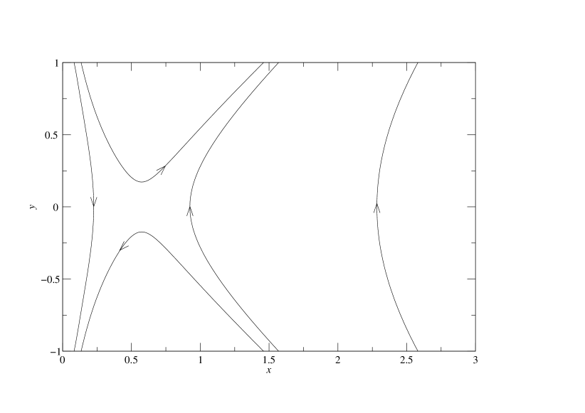
Figure 4: The phase portrait of system (55) with the cosmological constant but without global rotation $\Omega_{\omega,0}=0$. The acceleration region is situated on the left from the saddle point. Therefore, the recollapsing and then expanding models lie permanently in the acceleration domain. The Eddington model also belongs to this region. The Lemaître-Eddington type models with characteristic loitering phase start accelerating in the middle of quasi-static phase.

Figure 5: The phase portrait of the model (59) with global rotation $\Omega_{\omega,0}\neq 0$, the cosmological constant and dust in the projective coordinates $(v,u)\colon v=1/x$, $u=y/x$. By introducing such coordinates we can observe their behaviour at infinity. There are two types of trajectories which expand to the maximum scale factor and then recollapse and vice versa. In the first type of evolution the closed models start with the singularity $a(0)=0$ and $\dot{a}=0$, then reach the maximum radius and recollapse while the other class of models recollapse from $a(0)=\infty$ and $\dot{a}=-\infty$ to the minimum value of a, and then expand to infinity. In the generic case trajectories start from the anti-de Sitter stage and land at the de Sitter state.

VII The flatness and lambda problems

If we choose the standard FRW cosmology without the global rotation then the conservation equation for perfect fluid (3), satisfying the equation of state $p_{i}=(\gamma_{i}-1)\rho_{i}$, gives $\rho_{i}\propto a^{-3\gamma_{i}}$ and the $\rho/3$ term, in the Friedmann first integral (called also the Friedmann equation). Let us consider first these problems by setting $\Lambda=0$,

$$\frac{\dot{a}^{2}}{a^{2}}=-2V(a)=\frac{\rho_{0}}{3}a^{-3\gamma}+\frac{2}{3}\frac{\omega_{0}^{2}a^{6\gamma-10}}{(3\gamma-4)}+\frac{k}{a^{2}}$$ (60)

where $\sigma_{0}=0$, i.e., shear vanishes.

The matter term dominates the curvature term $ka^{-2}$ at large as long as the matter stress obeys $\rho+3p<0$, $\rho+p\geq 0$, that is if $0\leq\gamma<2/3$. This is what we describe as the flatness problem. Since the scale factor then evolves as $a(t)\propto t^{2/3\gamma}$ if $\gamma>0$ or if $\gamma=1$ as $\exp(H_{0}t)$. We can observe that it grows faster than the proper size of the particle horizon scale ($\propto t$) so long as $\gamma<2/3$. Therefore, a sufficiently long period of evolution during which expansion is dominated by matter with negative pressure with $\rho+3p<0$ can solve the flatness and horizon problems. Such a period of accelerated expansion is called inflation Barrow99b . However, as Barrow noted there is a flatness problem if the cosmological constant is added to the right hand side of the Friedmann equation. Then, to explain why it does not dominate matter term $\rho/3$ (at large $a(t)$) it is assumed that there exists the period in the early evolution of the universe during which weak energy condition for the matter is broken, i.e, $\rho+p<0$. This is what Barrow called the cosmological constant problem. For the standard FRW model the existence of corresponding $\gamma<0$ from equations of state mean that $\dot{a}<0$ which is the case of phantoms. Therefore, models with global rotation provide a solution of the flatness problem. It is formally equivalent to presence in the model some fictitious additional noninteracting fluid which obeys the equation of state $p_{\omega}=\frac{7-6\gamma}{3}\rho_{\omega}$, $\rho_{\omega}=\rho_{\omega_{0}}\left(\frac{a}{a_{0}}\right)^{6\gamma-10}$, $\rho_{\omega_{0}}=\frac{2}{3\gamma-4}\omega_{0}^{2}$. Then both weak and strong energy conditions for pure “rotational fluid” means

$$\rho_{\omega}+p_{\omega}=w_{\omega}\rho_{\omega}=\frac{10-6\gamma}{3}\rho_{\omega}\geq 0$$

$$\rho_{\omega}+3p_{\omega}=2\rho_{\omega}(4-3\gamma)\geq 0.$$

In the special case of dust matter we have inequality if the above conditions are violated

$$\rho_{\omega}+p_{\omega}=\frac{4}{3}\rho_{\omega}<0, \rho_{\omega}=\rho_{\omega_{0}}x^{-4}$$

$$\rho_{\omega}+3p_{\omega}=2\rho_{\omega}<0, \rho_{\omega_{0}}=-2\omega_{0}^{2},$$

i.e., both energy conditions are violated.

Finally, the strong and weak energy conditions for density energy of dust and rotational fluids requires respectively

$$(\rho_{\text{m}}+\rho_{\omega})+3p_{\omega}=\rho_{\text{m},0}a^{-3}\left(1-\frac{2}{\rho_{\text{m},0}}\omega_{0}^{2}a^{-1}\right)\geq 0,$$

$$(\rho_{\text{m}}+\rho_{\omega})+p_{\omega}=\rho_{\text{m},0}a^{-3}\left(1-\frac{8}{3\rho_{\text{m},0}}\omega_{0}^{2}a^{-1}\right)\geq 0.$$

Thus, during the evolution, first, the strong energy condition is violated for $a<\frac{2}{\rho_{\text{m},0}}\omega_{0}^{2}=\frac{2}{3H^{2}_{0}}\frac{1}{\Omega_{\text{m},0}}$ and the weak one is violated for $a<\frac{8}{3\rho_{\text{m},0}}$. We can also find the interval ${2\rho_{0}}<a<\frac{8}{3\rho_{\text{m},0}}\omega_{0}^{2}$ in which the strong energy condition is violated, whereas weak energy condition is still satisfied. It is possible because $\rho_{\omega}$ is negative. These are sufficient conditions to solve the flatness problem.

Because of the existence of the period in which $\rho+p<0$ (phantom), the cosmological constant problem can be solved and $\dot{a}<0$ is an unnecessary requirement. Unfortunately, the future horizon problem cannot be solved and the corresponding condition $\gamma\leq 2/3$ is identical to that of the solution of the horizon (or flatness) problem in the case with vanishing rotation.

Let us note that if we consider the case of the non-zero $\Lambda$ term, that is contributed by a pressure $p_{\Lambda}=-\rho_{\Lambda}$ then $\Lambda$ term on the right-hand side of (60) falls off faster than the curvature and matter density terms so long as $\gamma<2/3$ and $\gamma<0$ respectively. The contribution term from the global rotation falls off faster then curvature $\Lambda$ and matter density term so long as $\gamma<4/3$ (radiation), $\gamma<5/3$, $\gamma<10/9$, respectively.

Therefore, the cosmological constant term $\Lambda$, curvature term is proportional to $a^{-2}$ and term connected with global rotation falls off faster than $8\pi G\rho/3$ term in the FRW equation at large $a(t)$ if respectively $\gamma<0$ and $\gamma<2/3$ and $\gamma<10/9$, i.e., $\gamma<0$.

VIII Homologous universe and its angular momentum

In this section we demonstrate how Wesson’s argument can be generalised and how it works in our case Wesson79 ; Wesson83 . Wesson argued that because the dynamics of a gravitationally bound rotating system admits self similarity group of symmetry the relation between angular momentum $J$ of a astronomical system and its mass $J\sim M^{2}$ can be constructed due to constancy of the invariants of this kind of symmetry. In this section we demonstrate how Wesson’s argument can be generalised and how it works in our case. We generalise Wesson’s argumentation to the case of universe dynamics by consideration of Lie (continuous) symmetries of the FRW models with rotation. The Lie group theory of symmetries analysis gives us information about the group of symmetry transformations admissible by the differential equation structure. They preserve the structure of basic dynamical equations. In the set of solutions, the action of an admissible group includes a certain algebraic structure which can be used to find a family of new solutions from the known ones Barenblatt96 ; Bluman89 ; Stephani89 ; Ovsiannikov82 .

As is well known Kippenhahn80 , the new solution for the system equation, describing the static stars (in Newtonian as well as in General Relativity), can be obtained from the known ones through the homologous transformation Collins77 ; Biesiada88 ; Biesiada88b . We can find the homologous transformation of the symmetry type (i.e., preserving structure of differential equations) for the considered dynamics of the FRW model with rotation. It would be useful to rewrite basic dynamical equations (9) and (3) to the form in which instead of ($H$, $\rho$, $\omega$) variables we have ($a$, $\rho$, $\omega$). Then we obtain

$$\frac{da}{dt} =\sqrt{\frac{\rho a^{2}}{3}-k-\frac{2}{3}\omega^{2}a^{2}}$$ (61a)

$$\frac{d\rho}{dt} =-2\gamma\rho\sqrt{\frac{\rho a^{2}}{3}-k-\frac{2}{3}\omega^{2}a^{2}}a^{-1}$$ (61b)

$$\frac{d\omega}{dt} =-\omega(5-3\gamma)\sqrt{\frac{\rho a^{2}}{3}-k-\frac{2}{3}\omega^{2}a^{2}}a^{-1}.$$ (61c)

Now let us consider the differential equations system

$$\frac{du^{i}}{dx}=f^{i}(x,u^{1},\ldots,u^{m}),\quad i=1,\ldots,m,$$

and here the space of independent variable is denoted as $x$, dependent one $u^{\alpha}$ and its first derivatives, say $u^{\alpha^{\prime}}(\alpha=1,\ldots,m)$. The action of the Lie group $G$ of point transformation in the space $(x,u)$ is described by an infinitesimal operator $\mathcal{X}$—a generator of the symmetry

$$\mathcal{X}=\zeta(x,u^{1},\ldots,u^{m})\frac{\partial\phantom{x}}{\partial x}+\sum\limits_{i=1}^{m}\eta^{i}(x,u^{1},\ldots,u^{m})\frac{\partial\phantom{u^{i}}}{\partial u^{i}}.$$

The point transformation generated by $\mathcal{X}$ is called homologous if $\zeta=ax$ and $\eta^{i}=g^{i}u^{i}$, where $a,g^{i}(i=1,\ldots,m)$ are constants. Of course, if $\mathcal{X}\equiv\lambda^{s}(u)\partial_{s}$, then the finite transformation of symmetry $u\to\bar{u}$ are given as a solution of equation $\frac{d\bar{u}^{s}}{dt}=\lambda^{s}(u)$ with the initial conditions $\bar{u}^{s}(\tau=0)=u^{s}$ ($s=1,\ldots,m$). The action of the Lie group transformation can be extended from the ($x,u$) space to the ($x,u,u^{\prime}$) space, i.e for the first derivatives. On the other hand, $s$-th order (ordinary or partial) differential equation

$$F(x,u(x),u^{1}(x),\ldots,u^{s}(x))=0$$

defines a certain manifold $\mathcal{M}$ in the space ($x,u,u^{1},\dots,u^{s}$). We say that $F$ is invariant with respect to the action group $G$, provided that manifold $\mathcal{M}$ is a fixed point with respect to the $s$-th extension of $G$, i.e., $G^{s}(\mathcal{M})=\mathcal{M}$. In the terms of the infinitesimal operator it means that

$$\mathcal{X}^{s}F|_{F=0}=0$$

where $\mathcal{X}^{s}$ is the extented operator on the first derivatives

$$\mathcal{X}^{s}=\mathcal{X}+\zeta_{i}^{\alpha}(x,u,u^{\prime})\frac{\partial\phantom{u^{i}}}{\partial u_{i}^{\alpha}},\qquad u_{i}^{\alpha}=\frac{\partial u^{\alpha}}{\partial x^{i}},$$

$$\zeta_{i}^{\alpha}=D_{i}(\eta^{\alpha})-u_{j}^{\alpha}D_{j}(\zeta^{j}),\qquad D_{i}=\frac{\partial\phantom{x^{i}}}{\partial x^{i}}+u_{i}^{\alpha}\frac{\partial\phantom{u^{a}}}{\partial u^{\alpha}}.$$

The prolonged operators, which are generators of symmetry of equations in the space $(x,u)$, form the structure of a Lie algebra of the fundamental group.

The Lie method adopted to our case gives us the symmetry operator in the form

$$\mathcal{X}=\alpha\rho\frac{\partial}{\partial\rho}-\frac{\alpha}{2}a\frac{\partial}{\partial a}+\frac{\alpha}{2}\omega\frac{\partial}{\partial\omega}-\frac{\alpha}{2}t\frac{\partial}{\partial t},$$ (62)

where $\alpha=\text{const}$, i.e., the most general form of symmetries constitutes a homologous transformation. For our further analysis it is useful to introduce the notion of invariants of symmetry operator $\mathcal{X}$. For the infinitesimal operator $\mathcal{X}$ there is $m$ independent invariants which are solutions of the following system

$$\frac{dx}{\zeta(x,u^{1},\ldots,u^{m})}=\frac{du^{1}}{\eta^{1}(x,u^{1},\ldots,u^{m})}=\cdots=\frac{du^{m}}{\eta^{m}(x,u^{1},\ldots,u^{m})}.$$ (63)

In our case we can recover two invariants in the form

$$J_{1}=\rho a^{2},\qquad J_{2}=\omega a.$$ (64)

They exactly correspond to Wesson’s invariants expressed in dimensionless form $\eta_{1}\equiv G\rho a^{2}/c^{2}$, $\eta_{2}\equiv\omega a/c$. The significance of the obtained invariant homologous transformation of (45) is the following.

1) They can be used as good new variables to integrate the system by lowering its dimension. Then we obtain

$$\frac{dJ_{1}}{d\eta}=(2-3\gamma)J_{1},\qquad\frac{dJ_{2}}{d\eta}=(3\gamma-4)J_{2},\qquad\eta\colon Hdt=d\eta.$$ (65)

2) The invariant can be used to obtain a new solution from the known ones using the homologous theorem. If $a(t)$ is a solution of (45), then because $a(t)t^{-1}$ is invariant, $a(e^{-\alpha\tau/2}t)(e^{-\alpha\tau/2}t)^{-1}=\text{const}$ is also a solution, where the finite transformations are given in the form

$$\rho\to\bar{\rho}=\rho e^{\alpha\tau},\quad a\to\bar{a}=ae^{-\alpha\tau/2},\quad\omega\to\bar{\omega}=\omega e^{\alpha\tau/2},\quad t\to\bar{t}=e^{-\alpha\tau/2}$$ (66)

where $\tau$ is a group parameter and $\alpha=\text{const}$. Let us note that the finite transformation (66) preserves the angular momentum form

$$J=\rho a^{5}\omega=\bar{\rho}\bar{a}^{5}\bar{\omega},$$ (67)

i.e., this relation is invariant with respect to the homologous (or self similarity) transformation group given by (66). Physically the existence of this type of symmetry always means that a basic dynamical equation can be formulated in a dimensionless form.

It is interesting that (67) can be expressed in terms of invariants by

$$J=\frac{J_{2}}{J_{1}}M^{2},$$ (68)

and astrophysical relation $J\sim M^{2}$ which is closely obeyed over mass range $10^{18}g$ to $10^{48}g$ can be extended to the Universe, together with the Wesson’s philosophy that self similarity transformation plays an important role in astrophysics. This notion was introduced in astrophysics by Rudzki Rudzki02 . We note that it can play an important role in cosmology (see also Stephani89 ).

Moreover the ratio $J_{2}/J_{1}$ in the equation (68) is constant in the distinguished case of dust matter ($\gamma=1$). Therefore, there is no need for additional arguments which usually are taken from the astronomical observation about the constancy $J_{2}/J_{1}$ as in the Wesson argumentation because after integration of (65) we obtain immediately

$$\frac{J_{2}}{J_{1}}\sim e^{6(1-\gamma)\eta},$$ (69)

and only for $\gamma=1$ (dust) we obtain

$$\frac{J_{2}}{J_{1}}=\mbox{const}.$$ (70)

IX Conclusion

In this paper we studied the dynamics of the FRW universe with global rotation. Our approach is simplest in that we formulate the dynamical problem in two-dimensional phase space. Moreover, we find the Hamiltonian formulation of the dynamics. Such visualisation has a great advantage because it allows us to analyse the acceleration problem in a clear way. Due to the existence of the Hamiltonian constraint, it is possible to make the classification of the qualitative evolution paths by analyzing the characteristic curve which represents the boundary equation in configuration space. Dynamical system methods gives us all evolutional paths for all possible initial conditions. On the other hand, the representation of dynamics as a one dimensional Hamiltonian flow allows us to make the classification of the possible evolution paths in the configuration space. When we consider the dynamics of the FRW models with global rotation, a two-dimensional dynamical system in general, then there is a simple test of structural stability of the system (a dynamical system $S$ is said to be structurally stable if dynamical systems in the space of all dynamical system which are close to $S$ are topologically equivalent (physically realistic models on the plane should be structurally stable). Namely, if the right-hand sides of dynamical systems are in polynomial form, the global phase portraits are structurally stable on $S^{2}$ ($R^{2}$ with adjoint a Poincaré sphere) if, and only if, the number of critical points and limit cycles is finite, each point is hyperbolic and there are no trajectories connecting saddle points. Our conclusion is that the FRW models with global rotation are structurally stable, i.e., following Peixoto’s theorem dynamical systems with rotation form open and dense subsets in the space of all dynamical system on the plane. From the point of view of science modelling they are better and more adequate description of the observed universe than the FRW model without the cosmological term.

Our formalism gives natural base to express dynamical equations in the form of the FRW model with some additional fictitious noninteracting multifluid which mimics the effects of global rotation. It satisfies in the generic case the equation of state for radiation with some unusual negative energy density. We find basic dynamical equations describing the dynamics in the form of two-dimensional Hamiltonian dynamical systems in which coefficients are just dimensionless observational density parameters $\Omega_{i,0}$.

We also showed that global rotation produces a dark energy component but the cosmological term is still required to explain SNIa data. We also demonstrates how classical cosmological problems can be solved due to the existence of global rotation. We also derive the observationally suggested relation between the angular momentum and mass of the object $J\propto M^{2}$ from the property of self similarity of dynamics of the FRW cosmology with rotation.

The presented formalism forms the base for our further analysis of the magnitude redshift relation and finding the best fitting for $\Omega_{\omega,0}$ from recently available SNIa data and X-ray gas measurements of mass fraction in clusters of galaxies or measurements of angular size of radiogalaxies.

- (1) Y. N. Obukhov, T. Chrobok and M. Scherfner, Phys. Rev. D. 66, 043518, (2002), eprint gr-qc/0206080.
- (2) K. Lanczos, Z. Phys. 21, 73, (1924)
- (3) G. Gamov, Nature 158, 549, (1946)
- (4) K. Goedel, Rev. Mod. Phys. 21, 447, (1949)
- (5) S. W. Hawking, Mon. Not. R. Astr. Soc. 142, 129, (1969)
- (6) C. B. Collins and S. W. Hawking, Mon. Not. R. Astr. Soc. 162, 307, (1973)
- (7) J. D. Barrow, R. Juszkiewicz and D. Sonoda, Mon. Not. R. Astr. Soc. 213, 917, (1985)
- (8) E. F. Bunn, P. Ferreira and J. Silk, Phys. Rev. Lett. 77, 2883, (1996), eprint astro-ph/9605123.
- (9) A. Kogut, G. Hinshaw and A. Banday, Phys. Rev. D 55, 1901, (1997), eprint astro-ph/9701090.
- (10) O. Heckmann and E. Schücking, in Handbuch der Physik, edited by S. Flügge Springer-Verlag, Berlin (1959), vol. LIII, 489
- (11) O. Heckmann, Astron. J. 66, 205, (1961)
- (12) P. Szekeres and R. Rankin, Australian Math. Soc. B 20, 114, (1977)
- (13) J. M. M. Senovilla, C. F.Sopuerta and P. Szekeres, Gen. Rel. Grav. 30, 389, (1998), eprint gr-qc/9702035.
- (14) W. Godlowski, M. Szydlowski, P. Flin and M. Biernacka, Gen. Relat. Grav. 35, 907, (2003), eprint astro-ph/0404329.
- (15) A. R. King and G. F. R.Ellis, Commun. Math. Phys. 31, 209, (1973)
- (16) A. K. Raychaudhuri, Theoretical Cosmology Clarendon Press, Oxford, (1979)
- (17) G. F. R. Ellis, in Cargèse Lectures in Physics, ed. by E. Schatzman, Gordon and Breach New, York (1973), vol.6
- (18) L.-X. Li, Gen. Relat. Grav. 30, 497, (1998), eprint astro-ph/9703082
- (19) J. D. Barrow and C. G. Tsagas, Class. Quantum Grav. 21, 1773, (2004), eprint gr-qc/0308067.
- (20) P. Birch, Nature 298, 451, (1982)
- (21) E. S. Phinney and R. L. Webster, Nature, 301, 735, (1983)
- (22) M. F. Bietenholz and P. P. Kronberg, Ap. J. 287, L1, (1984)
- (23) M. L. Fil’chenkov, in Frontiers of Particle Physics, ed. A. Studenikin, World Scientific, Singapore (2003), 284
- (24) J. Silk, Mon. Not. R. Astr. Soc. 147, 13, (1970)
- (25) A. Djorgovski, in Nearly Normal Galaxies, ed. S. M. Faber, Springer Verlag, New York, (1987), 227
- (26) P. Flin and W. Godlowski, Mon. Not. R. Astr. Soc. 222, 525, (1986)
- (27) N. Kashikawa and S. Okamura, PASJ 44, 493, (1992)
- (28) W. Godlowski, Mon. Not. R. Astr. Soc. 265, 874, (1993)
- (29) W. Godlowski, Mon. Not. R. Astr. Soc. 271, 19, (1994)
- (30) S. Perlmutter et al., Nature 391, 51, (1998), eprint astro-ph/9712212.
- (31) S. Perlmutter et al., Ap. J. 517, 565, (1999), eprint astro-ph/9812133.
- (32) P. M. Garnavich et al., Ap. J. Lett. 493, L53, (1998), eprint astro-ph/9710123.
- (33) A. G. Riess et al., Astron. J. 116, 1009, (1998), eprint astro-ph/9805201.
- (34) W. Godlowski and M. Szydlowski, Gen. Relat. Grav. 35, 2171, (2003), eprint astro-ph/0303248.
- (35) I. Ciufolini and J. A. Wheeler, in Gravitation and Inertia, Princeton University Press, Princeton, (1995)
- (36) W. Godlowski and M. Szydlowski, Gen. Relat. Grav. 36, 767, (2004), eprint astro-ph/0404330.
- (37) G. F. R. Ellis and H. Van Helst, in: Theoretical and Observational Cosmology, eds Marc Lachièze-Rey, NATO Science Series Vol 541, (1998)
- (38) M. Dabrowski and J. Stelmach, Astron. J. 92, 1272, (1986)
- (39) H. P. Robertson, Rev. Mod. Phys. 5, 62, (1933)
- (40) M. Dabrowski, Annals Phys. (N.Y) 248, 199, (1996), eprint gr-qc/9503017.
- (41) S. Weinberg, Gravitation and Cosmology, Wiley, New York, (1972)
- (42) P. J. E. Peebles and B. Ratra, Rev. Mod. Phys. 75, 559, (2003), eprint astro-ph/0207347.
- (43) J. D. Barrow, Phys. Rev. D 59, 043515, (1999)
- (44) G. I. Barenblatt, Scaling, Self-similarity, and Intermediate Asymptotes Cambridge University Press, New York, (1996)
- (45) G. W. Bluman and S. Kumei, Symmetries and Differential Equations, Springer-Verlag, New York, (1989)
- (46) H. Stephani, Differential Equations, Their Solution Using Symmetries, Cambridge University Press, New York, 1989
- (47) L. V. Ovsiannikov, Group Analysis of Differential Equations Academic Press, New York, (1982)
- (48) P. S. Wesson, (Astron. Astroph. 80, 269 (1979)
- (49) P. S. Wesson, Astron. Astroph. 119, 313, (1983)
- (50) R. Kippenhahn, Stellar Structure and Evolution, Springer-Verlag, Berlin, (1980)
- (51) C. B. Collins, J. Math. Phys. 18, 134 (1977)
- (52) M. Biesiada, Z. Golda and M. Szydlowski, J. Phys. A 20, 1313 (1988)
- (53) M. Biesiada and M. Szydlowski, J. Phys. A 21, 3409, (1988)
- (54) A. Rudzki, Bull. Astroph., 19 134, (1902)