Hydrodynamical simulations of the jet
in the symbiotic star MWC 560

We performed hydrodynamical simulations with and without radiative cooling of jet models with parameters representative for the symbiotic system MWC 560. For symbiotic systems we have to perform jet simulations of a pulsed underdense jet in a high density ambient medium. We present the jet structure resulting from our simulations and calculate emission plots which account for expected radiative processes. In addition, our calculations provide expansion velocities for the jet bow shock, the density and temperature structure in the jet, and the propagation and evolution of the jet pulses.

In MWC 560 the jet axis is parallel to the line of sight so that the outflowing jet gas can be seen as blue shifted, variable absorption lines in the continuum of the underlying jet source. Based on our simulations we calculate and discuss synthetic absorption profiles.

Based on a detailed comparison between model spectra and observations we discuss our hydrodynamical calculations for a pulsed jet in MWC 560 and suggest improvements for future models.

1 Introduction

Jets are very common in a variety of astrophysical objects on very different size and mass scales. They can be produced by supermassive black holes in the case of Active Galactic Nuclei (AGN), by stellar black holes in Black Hole X-ray Binaries (BHXBs), by neutron stars in X-ray Binaries, by pre-main sequence stars in Young Stellar Objects (YSO) and by white dwarfs in supersoft X-ray sources and in symbiotic binaries. Jets in symbiotic systems are not yet as well investigated theoretically as the other objects. Due to the fact, that their parameters are in a different regime, studying them should promise new insights. The density contrast $\eta=\rho_{\rm{jet}}/\rho_{\rm{ambient}}$ is about $10^{-3}-10^{-2}$ in symbiotic stars ($1-10$ in YSO, $\approx 0.1$ in AGN), the outflow velocities are with 1000-5000 km s^-1 somewhat higher than in YSOs with $100-1000$ km s^-1 ($\approx c$ in AGN). The absolute densities of ${\rm N}_{e}\approx 10^{6}-10^{8}$ cm^-3 are similar to YSO jets. However, the jet gas densities in symbiotic systems are the highest for underdense jets ($\eta<1$) – which are in AGN jets smaller than $10^{-2}$ cm^-3 – therefore radiative processes become very important.

Symbiotic systems consist of a red giant undergoing strong mass loss and a white dwarf. More than one hundred symbiotic stars are known, but only about ten systems show jet emission. The most famous systems are R Aquarii, CH Cygni and MWC 560. While the first two objects are seen at high inclinations – a fact which makes it possible to study the morphology and structure of jets of symbiotic stars – the jet axis in MWC 560 is practically parallel to the line of sight. This special orientation provides the opportunity to observe the outflowing gas as line absorption in the source spectrum. With such observations the radial velocity and the column density of the outflowing jet gas close to the source can be investigated in great detail. In particular we can probe the acceleration and evolution of individual outflow components with spectroscopic monitoring programs as described in Schmid et al. (2001).

MWC 560 is a symbiotic binary system with a late M giant undergoing strong mass loss. At least a significant fraction of the lost material is accreted by the companion, which is as for most symbiotic stars a white dwarf. No radial velocity variation have been detected for the red giant most likely because the inclination of the system is close to $0^{\circ}$. The orbital period of the system is not known. However, Schmid et al. (2001) provide arguments for a likely orbital period in the range 4 to 10 years.

We performed hydrodynamical simulations with and without cooling of jets with parameters that are intended to represent those in MWC 560. In a grid of eight simulations we investigated the influence of different jet pulse parameters. Due to the high computational costs of simulations including cooling, this grid was restricted to adiabatic simulations. Existing simulations of pulsed jets for YSO systems (e.g. Stone & Norman 1993; Steffen et al. 1997; de Gouveia dal Pino & Cerqueira 2002, and references therein) showed that the resulting jet structure differs strongly between purely hydrodynamical models and models using radiation hydrodynamics. Therefore, one model simulation was performed which includes a treatment of radiative cooling. We calculate from these models the absorption line profiles and investigate their ability to explain the corresponding spectroscopic observations.

Due to the fact that morphological studies of the jet structure and synthetic emission plots are the first model results which are obtained, we also present them in this paper. In addition, our calculations provide expansion velocities for the jet bow shock, the density and temperature structure in the jet, and the propagation and evolution of the jet pulses. This allows us to compare at least the qualitative properties of the jet simulations with various types of observations of jets in symbiotic systems.

In section 2, we summarize the main observational results of the jet sources in symbiotic systems and in particular for the jet absorptions in MWC 560. A detailed description of our hydrodynamic model is given in section 3. The resulting jet structures are described and emission plots are presented (section 4). In section 5, we discuss the model parameters which define the synthetic absorption line profiles and the results for different model cases. Section 6 describes the temporal evolution of the high velocity gas in the pulses and compares the resulting jet absorption profiles with observation. Finally a summary and a discussion are given.

2 MWC 560 and jets in symbiotic stars

Symbiotic binaries are a very heterogeneous class of objects, showing different types of nova-like activity. Jets are only expected in systems with substantial accretion from the red giant via a disk. The presence of a disk can be inferred from strong, short term ($\sim$ hour) flickering of the hot component. However, flickering is only observed in very few objects (Sokoloski, Bildsten & Ho 2001). In many systems an accretion disk may be present, but it is hard to observe due to the much stronger emission from the cool giant, the nebula or the accreting white dwarf. Further the disk may be hidden by a larger scale circumbinary disk. In some systems the jet emission seems to be a transient phenomenon (e.g. Tomov, Munari & Marrese 2000), connected with an active phase of the hot component - perhaps due to an accretion disk instability. However, such transient features are difficult to study observationally.

2.1 MWC 560

The jet in the symbiotic system MWC 560 serves in this study as template object for our model calculations. We have chosen this unique jet system because it provides us with direct information on some hydrodynamical parameters of the jet gas in the near vicinity $<1$ AU of the jet source.

MWC 560 is observationally a point source. In early 1990, MWC 560 attracted attention with a photometric outburst of 2 mag. With spectroscopic observations it was found that the system exhibits strongly variable, blue shifted absorptions with outflow velocities (RV) up to 6000 km s^-1 (Tomov et al. 1990). Unlike in normal P Cygni profiles from a stellar wind the blue absorption components are detached from the emission component. After the initial outburst phase the outflow showed during about a year a low velocity phase with $v=300\,{\rm km}\,{\rm s}^{-1}$. Since September 1991, the “normal” outflow mode is re-established, with strongly variable, detached absorption components and a typical outflow velocity of $\approx$ 1500 km s^-1 (Tomov & Kolev 1997). The absorption line structure can be explained as a jet outflow whose axis is parallel to the line of sight (Tomov et al. 1990; Schmid et al. 2001). This very special system orientation is supported by the absence of measurable radial velocity variations for the red giant indicating that the orbital plane and therefore presumably also the accretion disk are perpendicular to the line of sight. Moreover strong flickering is present (Sokoloski, Bildsten & Ho 2001) as expected for an accretion disk of a strong jet source seen pole on. Up to now, this object is the only stellar object known with this special jet orientation. Therefore MWC 560 is most useful for studying the acceleration and dynamical evolution of small scale structures in a stellar jet. Studying the variable gas absorptions yields information about the outflowing gas at very small distances $<10$ AU from the source.

A most important observational source of information for the investigation of the pulsed jet in MWC 560 are the monitoring observations described in Schmid et al. (2001). Figure 1 displays a small fraction of the H$\delta$ jet absorption data obtained during this campaign. It is clearly visible that the jet absorptions in MWC 560 are very different from classical P Cygni profiles of stellar winds. The variable absorption features can be grouped into three different components (see Fig. 1).

Figure 1: Time series for the H$\delta$ $\lambda$4102 jet absorption in MWC 560 from the campaign of Schmid et al. (2001). The sequence shows normalized spectra (and shifted for clarity) from days before and after the appearance of a strong high velocity component on day 144.

• The first component is relatively stable with RV of $\approx-1200\pm 300$ km s^-1. This component is saturated over a wide velocity range in the H i Balmer lines, while the metal lines (Na i, Fe ii, Ca ii) are not (or not completely) saturated and several subcomponents can be resolved. Focusing specifically on the Na i line, one notices that no absorptions with RV $\geq-1000$ km s^-1 are present. This shows that low velocity gas is at least partly ionized and produces no Na i absorptions.

• The second component are transient high-velocity absorptions which appear repeatedly on timescales of about a week. In Fig. 1 such a strong high velocity absorption appears on day 143 and is fully developed on day 144. For day 144 the maximum outflow velocity is about $2100$ km s^-1 while other high velocity components reach velocities up to $2600$ km s^-1 (days 181 and 193, see Schmid et al. 2001). These fast components can be seen in all H i lines and simultaneously in the metal lines. Particularly strong, compared to the stable component around $\approx-1200\pm 300$ km s^-1, are the high-velocity components in He i. The transient high velocity components reach their maximum velocity within one day and decay again in the following few days. The disappearance is faster in He i than in H i. The He i transitions have a higher excitation potential, therefore the He i features can be associated with hotter and/or higher ionized gas.

• The third absorption component in the RV range of $\approx-900$ to $-400$ km s^-1 weakens at the same time as the appearance of the high velocity component. In Fig. 1 the reduced absorption (enhanced emission) is particularly well visible for days 143 and 144 around $-900$ km s^-1. The low velocity absorptions are anti-correlated with the transient high velocity components. This is an indication for a close relationship between the acceleration region producing the low velocity absorption and the transient high velocity components.

The observations provide much more information on the jet structure in MWC 560 and we refer the interested reader to Schmid et al. (2001).

In that work, various jet parameters for MWC 560 were estimated from the observations.Of interest for this study on synthetic spectra from hydrodynamic models is the estimated jet mass outflow rate of $>7\times 10^{-9}\,{\rm M}_{\odot}\,{\rm yr}^{-1}$. In addition it was possible to derive values for the velocity and the gas density for the “normal” jet outflow, but also for phases with strong high velocity components. These determinations of hydrodynamical parameters of the initial jet gas in MWC 560 serve now in this paper as input parameter for the numerical simulations of pulsed jets in symbiotic systems.

The pole on orientation of the jet in MWC 560 has of course the drawback that this system is not suited for investigations on the morphological structure of the jet. For this we have to use observations of jets which are seen from the side.

2.2 R Aquarii and CH Cygni

R Aquarii is with a distance of about 200 pc one of the nearest symbiotic stars and a well known jet source. The system contains a Mira-like variable with a pulsation period of 387 days. The hot, ionizing companion is not resolved, but it is presumably a white dwarf or sub-dwarf with an accretion disk. An orbital period of $\approx 44$ years has been suggested, but this value is highly uncertain (Wallerstein 1986). The jet has been extensively observed in the optical, at radio wavelengths and with X-ray observations (e.g. Solf & Ulrich 1985; Paresce & Hack 1994; Hollis et al. 1985a, b; Kellogg, Pedelty & Lyon 2001). R Aqr shows a jet and a counter-jet extending about 10^′′ each. The jets are embedded in an extended and complex nebulosity. Individual jet features are morphologically and photometrically variable with time. In observations with HST (Paresce & Hack 1994), the jet can be traced down to a distance of only 15 AU from the Mira where it is already collimated with an opening angle of $<15{{}^{\circ}}$. After a straight propagation of 50 AU, it hits a dense clump and produces a radiative bow shock (feature N2; notation as in Paresce & Hack 1994). The flow seems to split into two parts: one stream extends around 700 AU towards feature A1, further a series of parallel features (N3 - N6) are detected downstream of N2, orthogonal to the original flow. HST observations taken at different epoch revealed that the transverse velocity (proper motion) of the different features increases from about 40 to 240 km s^-1 with increasing distance from the central jet (Hollis et al. 1985b). In Chandra images (Kellogg, Pedelty & Lyon 2001), the knots are not as well resolved as in optical observations. Only larger clumps are visible, corresponding to the central source, the feature A1 and the feature S3 in Paresce & Hack (1994). VLA observations (Hollis et al. 1985a) show similar structures.

For R Aqr a major problem for the interpretation of the jet observations is the blending of jet features with emission from the surrounding nebulosity. Therefore it is not clear whether the observed features are due to the jet gas, due to the ambient medium which is shock-excited by the jet outflow, or just circumstellar material ionized by the radiation from the accreting component.

CH Cygni is a symbiotic binary where the hot component shows strong, short term flickering as expected for a bright accretion disk. The cool companion is an extended M6 III giant with a radius of about 200 $\mbox{R}_{\odot}$. The binary period is 5700 d (Crocker et al. 2002) and eclipses of the flickering component indicate a system inclination near 90^∘ (Mikolajewski, Mikolajewska & Tomov 1987). In 1984/85, the system showed a strong radio outburst, during which a double-sided jet with multiple components was ejected (Taylor, Seaquist & Mattei 1986). This event enabled an accurate measurement of the jet expansion with an apparent proper motion of 1.1 arcsec per year. With a distance of 268 pc (HIPPARCOS) (Crocker et al. 2001), this leads to a jet velocity near 1500 km s^-1. The spectral energy distribution derived from the radio observations suggest a gas temperature of about 7000 K for the propagating jet gas (Taylor, Seaquist & Mattei 1986). In HST observations (Eyres et al. 2002), arcs can be detected which also could be produced by episodic ejection events. The X-Ray spectrum taken with ASCA (Ezuka, Ishida & Makino 1998) is composed of three components which are associated with the hot source and the secondary or the radio jet. X-Ray imaging is not yet available.

3 The numerical models

In the following, we describe the employed computer code with the incorporated equations, the model geometry and the chosen jet parameters. We also discuss the simplifications and approximations made due to the constraints set by the available computer resources.

3.1 The computer code

3.1.1 General description

With the code NIRVANA (Ziegler & Yorke 1997) we solve the following set of the hyperbolic differential equations of ideal hydrodynamics

$$\frac{\partial\,\rho}{\partial\,t}+\nabla\,(\rho\,{\bf v}) = 0$$

$$\frac{\partial\,(\rho\,{\bf v})}{\partial\,t}+\nabla\,(\rho\,{\bf v}\otimes{\bf v}) = -\nabla\,p-\rho\,\nabla\,\Phi$$ (1)

$$\frac{\partial\,e}{\partial\,t}+\nabla\,(e\,{\bf v}) = -p\,\nabla\,{\bf v}+\Lambda(T;\rho_{i})$$

$$p = (\gamma-1)\,e.$$

Thereby $\rho$ is the gas density, $e$ the energy density, ${\bf v}$ the velocity and $\gamma$ the ratio of the specific heats at constant pressure and volume. NIRVANA uses second order accurate finite-difference and finite-volume methods and explicit time-stepping.

This code was modified by M. Thiele (Thiele 2000) to calculate energy losses due to non-equilibrium cooling by radiative emission processes. The microphysics is introduced via the cooling term $\Lambda$ in the energy equation and the following interaction equations for the species. When cooling is important, the above equations are supplemented by a species network

$$\frac{\partial\,\rho_{i}}{\partial\,t}+\nabla\,(\rho_{i}\,{\bf v})=\sum_{i=1}^{N_{s}}\,\sum_{j=1}^{N_{s}}\,k_{ij}(T)\,\rho_{i}\,\rho_{j}$$ (2)

with $\rho_{i}$ the species densities satisfying $\rho=\sum_{i=1}^{N_{s}}\,\rho_{i}$ for the total density. $k_{ij}$ are the rate coefficients for two-body reactions which are functions of the fluid temperature $T$. They describe electron collision ionization and radiative and dielectronic recombination processes. The summations go over the $N_{s}$ species. Both atomic and/or molecular species can be included in the model and NIRVANA_C can handle up to 36 species (Thiele 2000).

In the optically thin case, the cooling rate is a function of the species densities and temperature, $\Lambda=\Lambda(T;\rho_{i})$ (Sutherland & Dopita 1993). Cooling functions describing electron collision ionization, radiative and dielectronic recombination and line radiation. When cooling is very efficient, the atomic network is solved in a time-implicit way (Thiele 2000). This code has been extensively tested in Thiele (2000) and Krause (2001).

When the cooling is solved dynamically with the full set of non-equilibrium equations, the various ionization states and concentration densities $\rho_{i}$ of each element are calculated from the atomic rate equations. They are used explicitly in the cooling functions as

$$\Lambda(T;\rho_{i})=\sum_{i=1}^{N_{s}}\,\sum_{j=1}^{N_{s}}\,e_{ij}(T)\,\rho_{i}\,\rho_{j}+\Lambda_{BS}(T)$$ (3)

with $e_{ij}$ the cooling rates from two-body reactions between species $i$ and $j$, and $\Lambda_{BS}$ the cooling function due to Bremsstrahlung. In this case, the equation of state has to be given in the form

$$T=\frac{\gamma-1}{k_{B}}\,\frac{e}{\sum_{i=1}^{N_{s}}\,n_{i}}.$$ (4)

The code in its present form can handle collisional excitation, collisional ionization, recombination, metal-line cooling and Bremsstrahlung.

3.1.2 Our cooling setup

The available computer resources set strong constraints to the microphysics which can be included in our models. Important for jet simulations is a high spatial resolution in order to resolve the fine structure.

The parameter study for pulsed jets is therefore restricted to adiabatic simulations, where we neglect both the cooling term $\Lambda$ in the energy equation in the set of equations (3.1.1) and the interaction equations (2).

In addition, one model simulation was performed which includes a simple treatment of radiative cooling. Instead of the full explicit cooling function $\Lambda(T;\rho_{i})$, we consider only cooling by hydrogen, together with a general non-equilibrium cooling function $\Lambda(T)$ adapted from Sutherland & Dopita (1993) – without radiation field and assuming solar abundances – to account for the cooling by the heavier elements. The cooling function neglects collisional de-excitation. For the temperature regime of our calculations T $>10000$ K collisional deexcitation is only of importance for densities above 10⁸ cm^-3. Thus in the jet regions with the highest densities our cooling rate may be slightly overestimated. This effect will most likely be more than overcompensated by the fact that the limited resolution of our calculations underestimates the gas density (clumping) and the cooling rate. For hydrogen we solve the atomic network of H i, H ii and e^- and calculate the cooling due to collisional ionization of H i and due to collisional excitation of hydrogen line emission. The abundances of the species follow from the assumed initial jet temperature of $10^{4}$ K and the total density (see below).

3.2 Geometric model

Due to high computational costs of our cooling treatment and in order to combine a large computational domain with high spatial resolution it was not possible to perform model simulations in three dimensions. Therefore we had to choose a two-dimensional slice of the full domain and to assume axisymmetry. This kind of simulation is often called 2.5D simulations. The geometry of this slice in the examined system is shown in Figure 2. The dimensions of this two-dimensional slice are set to 50 AU in polar direction perpendicular to the orbital plane of the binary and 30 AU in the direction of the orbital plane – Figure 2 is not drawn to scale.

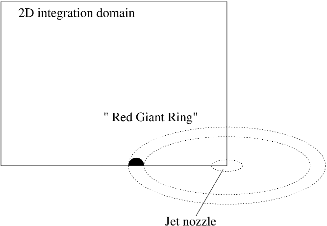
Figure 2: Sketch of the reduction from 3D to 2.5D simulations

The hot component is located in the origin of the coordinate frame, therefore the companion is expanded into a “Red Giant Ring”. In the 2D integration domain, only half of the cross-section of this ring on this slice is included. The binary separation in the models is chosen to 4 AU which is of the order of the estimated separations of 3.3 - 5.2 AU. The density of the red giant is set to $2.8\cdot 10^{-5}$ g cm^-3 and its radius to 1 AU.

Surrounding the red giant, a stellar wind is implemented. The wind has a constant velocity of $v=10$ km/s, a gas temperature of $T=50$ K and a mass loss of 10^-6 $\mbox{M}_{\odot}$ yr^-1. The density of the red giant wind at the surface of the star is then $2.2\cdot 10^{-14}$ g cm^-3. The density of the external medium is given by an $1/r^{2}_{\rm{rg}}$-law for a spherical wind where $r_{\rm{rg}}$ is the distance from the center of the red giant. The density of the red giant wind near the jet nozzle is about 200 times higher than the initial jet density. At a distance of 50 AU from the symbiotic system, i.e. at the end of the integration domain, the wind density is about equal to the jet density at the nozzle.

In 3D this density distribution corresponds for small z ($<5$ AU) to a torus-like structure which becomes for large z ($>10$ AU) a slightly flattened but quasi-spherical distribution $\approx 1/r^{2}$ centered on the jet nozzle. This seems to be a reasonable approximation for the z-direction. In the r-direction we introduce by this procedure artifically a density symmetry around the jet axis, which may be a qualitatively important difference compared to real jets in binary systems.

The gravitational potential of the two stars with assumed masses of 1 $\mbox{M}_{\odot}$ each is considered. However, the effect of the gravitational potential on the resulting jet structure is marginal.

The numerical resolution was chosen to 20 grid cells per AU, therefore our computational domain was 1000$\times$600 grid cells. To account for the counter-jet and the other part of the jet, respectively, the boundary conditions in the equatorial plane and on the jet axis are set to reflection symmetry. On the other boundaries, outflow conditions are chosen.

3.3 Parameters for the pulsed jet

The jet is produced within a thin jet nozzle with a radius of 1 AU. Because we like to investigate in these simulations the propagation of small scale structures in the jet and not the formation and collimation of the jet outflow, this ansatz is appropriate. We assume that the jet is already completely collimated when leaving the nozzle. To simulate the stable velocity component mentioned, the initial velocity of the jet is chosen to 1000 km s^-1 or 0.578 AU d^-1 and its density is set to $8.4\cdot 10^{-18}$ g cm^-3 (equal to a hydrogen number density of $5\cdot 10^{6}$ cm^-3). These parameters lead to a density contrast $\eta$ of $5\cdot 10^{-3}$, a Mach number of $\approx 60$ in the nozzle and a mass loss rate of $\approx 10^{-8}$ $\mbox{M}_{\odot}$ yr^-1.

Repeatedly each seventh day, the velocity and density values in the nozzle are changed to simulate the jet pulses which are seen in the observations of MWC 560. The effects of different pulse densities and speeds are investigated with a parameter study for adiabatic jet models.

4 Jet structure

4.1 Adiabatic models

We present eight adiabatic models for pulsed underdense jets which differ in their pulse parameters.

Table 1 lists the main parameters of the models: the model number, the density of the pulse in the nozzle n_pulse in cm^-3, the velocity of the pulse in the nozzle v_pulse in cm s^-1, the mass loss during the pulse $\dot{M}$ in g s^-1 and in $\mbox{M}_{\odot}$ yr^-1 and the kinetic jet luminosity during the pulse in erg s^-1. Each pulse lasts for one day. Thus the first 4 models have pulses with enhanced velocity and lower, the same or higher density as the “regular”outflow. In the models v to viii only the density is changed, except for the special model vii which has no pulses at all. Columns 7 and 8 in Table 1 give the axial and radial extent of the bow shock after 380 days of simulation time at which the first model (model iv) reaches the outer boundary. The bow shock sizes are results of our simulations which will be discussed below.

Table 1: Parameters of the jet pulses: the model number, the density of the pulse in the nozzle n_pulse in cm^-3, the velocity of the pulse in the nozzle v_pulse in cm s^-1, the mass outflow during the pulse $\dot{M}$ in g s^-1 and in $\mbox{M}_{\odot}$ yr^-1, the kinetic jet luminosity during the pulse in erg s^-1 and the axial and radial extent of the bow shock after 380 days of simulation time. Model vii is a special case, because no pulses are present. Therefore “pulse” values given for this model are identical to the jet parameters out of pulses valid for each model

model	npulse [cm-3]	vpulse [cm s-1]	$\dot{M}$ [g s-1]	$\dot{M}$ [$\mbox{M}_{\odot}$ yr-1]	Ljet [erg s-1]	$z_{\rm{b.\,s.}}$ [ AU ]	$r_{\rm{b.\,s.}}$ [ AU ]
i	$1.25\cdot 10^{6}$	$2.0\cdot 10^{8}$	$2.94\cdot 10^{17}$	$4.66\cdot 10^{-9}$	$5.88\cdot 10^{33}$	41.2	15.2
ii	$2.5\cdot 10^{6}$	$2.0\cdot 10^{8}$	$5.88\cdot 10^{17}$	$9.33\cdot 10^{-9}$	$1.18\cdot 10^{34}$	42.0	15.4
iii	$5.0\cdot 10^{6}$	$2.0\cdot 10^{8}$	$1.18\cdot 10^{18}$	$1.87\cdot 10^{-8}$	$2.35\cdot 10^{34}$	46.0	17.1
iv	$1.0\cdot 10^{7}$	$2.0\cdot 10^{8}$	$2.35\cdot 10^{18}$	$3.73\cdot 10^{-8}$	$4.70\cdot 10^{34}$	50.0	18.4
v	$1.25\cdot 10^{6}$	$1.0\cdot 10^{8}$	$1.47\cdot 10^{17}$	$2.33\cdot 10^{-9}$	$7.35\cdot 10^{32}$	43.8	14.4
vi	$2.5\cdot 10^{6}$	$1.0\cdot 10^{8}$	$2.94\cdot 10^{17}$	$4.66\cdot 10^{-9}$	$1.47\cdot 10^{33}$	48.6	14.6
vii$\,{}^{*}$	$5.0\cdot 10^{6}$	$1.0\cdot 10^{8}$	$5.88\cdot 10^{17}$	$9.33\cdot 10^{-9}$	$2.93\cdot 10^{33}$	48.0	14.4
viii	$1.0\cdot 10^{7}$	$1.0\cdot 10^{8}$	$1.18\cdot 10^{18}$	$1.87\cdot 10^{-8}$	$5.88\cdot 10^{33}$	38.7	14.5

^∗ equivalent to no pulses, these values represent the jet parameters out of pulses valid for each model

In Fig. 3 the logarithm of density is plotted for model i of the eight hydrodynamical models listed in Table 1. The density plots of the other seven simulations are qualitatively similar and therefore omitted.

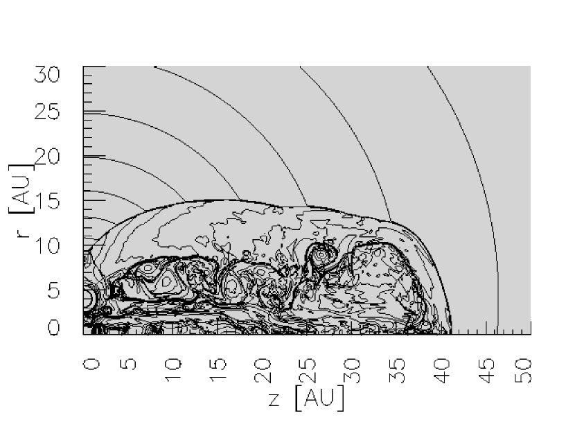
Figure 3: Contour plot of the logarithm of density at day 380; model i ($v_{\rm{pulse}}=2000$ km s^-1, $n_{\rm{pulse}}=1.25\cdot 10^{6}$ cm^-3)

In the models i–iv with the higher jet pulse velocity of 2000 km s^-1, the axial extent of the bow shock after 380 days – and therefore its averaged velocity – is increasing with increasing jet pulse density and mass outflow (see Table 1). This seems to be a trend in the simulations which is also valid for the radial extent of the bow shock. No clear trend is present in the four models v–viii, where the jet velocity is constant and only the jet pulse density is varied. The models with the highest and lowest pulse density have a lower averaged bow shock velocity than the intermediate models. The radial extent of the bow shock, however, is for all four models v–viii practically equal.

Thus we can say that the shock front expansion velocity is about equal within $10-20$ per cent for all our adiabatic jet simulations. The average expansion velocity of the bow shock during the first year is about $200\leavevmode\nobreak\ {\rm km}\,{\rm s}^{-1}$ in axial direction and about $75\leavevmode\nobreak\ {\rm km}\,{\rm s}^{-1}$ in radial direction. This has to be compared with the gas velocity in the jet nozzle, which is $1000\leavevmode\nobreak\ {\rm km}\,{\rm s}^{-1}$.

In the models, temperatures are present in the range of $10^{3}$ K in the red giant wind and $10^{5}$ - $10^{8}$ K in the jet (Fig. 4). These are by far too high for the observed absorptions from neutral or singly ionized metals which are only expected for cool gas with temperatures around $T\approx 10000$ K or lower.

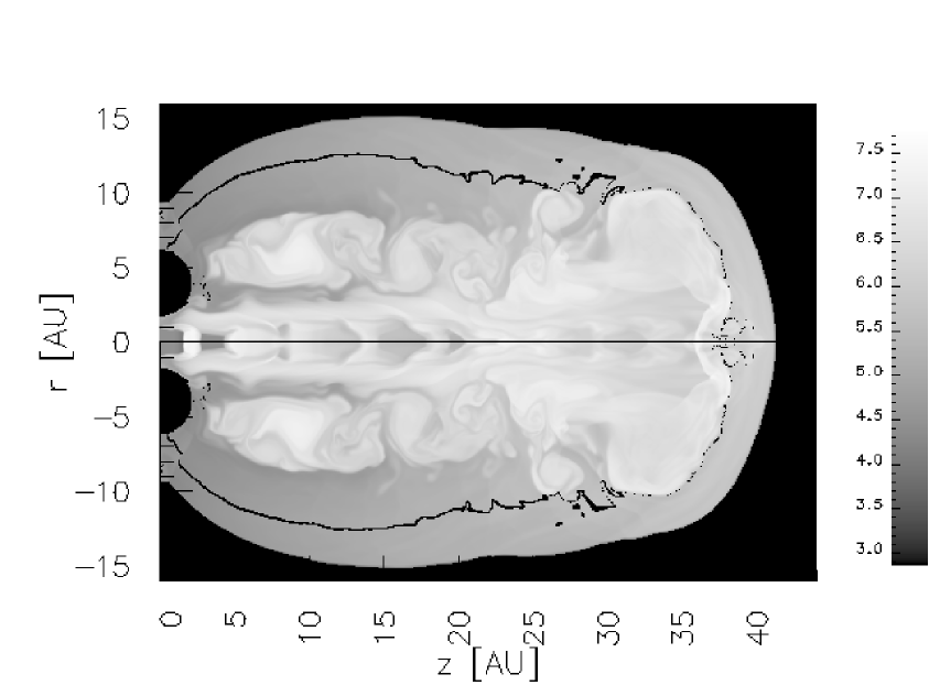
Figure 4: Logarithm of temperature of the model i; temperatures are present in the range of $10^{3}$ K in the red giant wind, of $10^{5}$ K in the shocked ambient medium and up to $10^{8}$ K in the jet beam and the cocoon; in this and the following color plots, only the jet material is considered which is filtered out by means of a passively advected tracer, the black line inside the jet cocoon is an artifact resulting from this filtering

It is well known from previous simulations of protostellar and extragalactic jets (e.g. Stone & Norman 1993; Steffen et al. 1997; de Gouveia dal Pino & Cerqueira 2002, and references therein) that the resulting jet structure differs strongly between purely hydrodynamical models and models using radiation hydrodynamics. This should also be the case in the parameter region of jets in symbiotic stars.

An estimate on the cooling time for the jet gas due to bremsstrahlung can be obtained from

$$t_{cool}=\frac{n\,k\,T}{1.68\cdot 10^{-27}\,T^{1/2}\,n_{e}\,n_{i}}=0.83\,\frac{\sqrt{T_{7}}}{n_{7}}\,\rm{yr}$$ (5)

where $T_{7}$ is the temperature in units of $10^{7}$ K which is about the postshock temperature of shocks with velocities of 1000 km s^-1 (Dopita & Sutherland 2003) and $n_{7}$ the number density in units of $10^{7}$ cm^-3, which are typical for our adiabatic models. It follows that the cooling time due to bremsstrahlung is comparable to the propagation time of the jet. This implies that radiative cooling is important for the employed jet model parameters and should be included in the energy equation.

4.2 Model with cooling

We performed one pulsed jet simulations including radiative cooling. For this we have chosen the same parameters as for the hydrodynamical model i, in which the jet velocity during the pulse phase is doubled from 1000 km s^-1 to 2000 km s^-1 while the particle number density is reduced by a factor of 4 from $5\cdot 10^{6}\,{\rm cm}^{-3}$ to $1.25\cdot 10^{6}\,{\rm cm}^{-3}$ in the jet beam. Thus the kinetic energy of the jet gas in the nozzle remains constant.

Radiative cooling is treated with a simple procedure. The cooling by metals is described by a general cooling function $\Lambda(T)$ adopted from Sutherland & Dopita (1993) and bremsstrahlung emission is considered. In addition we determined for each grid point the density of H i, H ii and e^- from the rate equations and calculate the cooling due to collisional ionization and line excitation of H i.

The expensive computational costs of the additional terms and equations to solve, together with an increased demand for memory, made it impossible to perform this simulation on a normal workstation. Therefore the already vectorized code was expanded to run on the NEC SX-5 supercomputer at the High Performance Computing Center (HLRS) in Stuttgart (Krause 2001).

Figure 5: Logarithm of temperature of the model i with cooling; again the highest temperatures are present in the cocoon and jet beam, the region of medium temperatures is shrinked with respect to model i without cooling

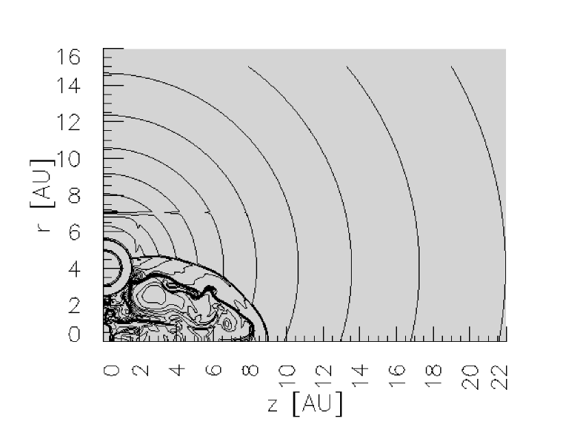
Figure 6: Contour plot of the logarithm of density at day 74; model i without cooling ($v_{\rm{pulse}}=2000$ km s^-1, $n_{\rm{pulse}}=1.25\cdot 10^{6}$ cm^-3)

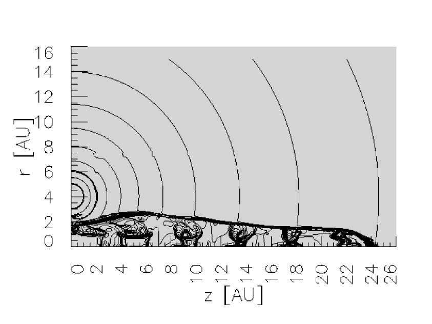
Figure 7: same as figure 6; model i with cooling ($v_{\rm{pulse}}=2000$ km s^-1, $n_{\rm{pulse}}=2.5\cdot 10^{6}$ cm^-3)

The cooled jet looses energy through radiation which instantaneously lowers the pressure and the temperature (Fig. 5). Therefore the radial extension of the jet, the cross section and the resistance exerted by the external medium are weakened. This leads to a faster propagation velocity. In Figs. 6 and 7, the jet density structure after 74 days is plotted for model i without and with cooling, respectively. This illustrates well the dramatic difference in the jet propagation. The bow shock velocity shows an apparently steady increase from about $500\leavevmode\nobreak\ {\rm km}\,{\rm s}^{-1}$ during the first days to about $730\leavevmode\nobreak\ {\rm km}\,{\rm s}^{-1}$ after 70 days. This steadiness, however, could be pretended by our coarse time resolution of 1 day. The average bow shock velocity for the covered 74 days is $570\leavevmode\nobreak\ {\rm km}\,{\rm s}^{-1}$. The bow shock velocity is increasing with time, because the jet head area remains almost constant and is therefore not able to compensate the decreasing local density contrast as in the simulations without cooling. The maximum radial extend of the jet cocoon is about 2.5 AU.

4.3 Jet structure

From our simulations we can investigate in detail the internal structure of the model jets. In Figs. 8-12 axial cuts along the jet of hydrodynamical quantities are plotted for model i without and with cooling. However, in the following discussion we focus on the calculations with radiative cooling. The cooled jet shows a very simple, periodic jet structure for the Mach number, axial velocity, density, pressure and temperature (Figs. 8-12). The internal shocks, which have not yet merged with the bow shocks, can be identified with well defined discontinuities in all parameters.

The jet flow shows thus two very different states of gas parameters which we call knots and hot beam. In the knots the density is high $\approx 10^{-16}\,{\rm g}\,{\rm cm}^{-3}$ and the temperature low $\approx 10^{4}$ K. Contrary to this the density in the hot beam is about 1000 times lower or $\approx 10^{-19}\,{\rm g}\,{\rm cm}^{-3}$ while the temperature is much higher between $10^{5.5}$ K to $10^{7}$ K.

Figure 8: Cut of the logarithm of Mach number along the jet axis for model i with cooling and without cooling. Results for both models are for day 74 in the simulation, for which 2D plots are plotted in Figs. 6 and 7 respectively.

Figure 9: Cut along the jet axis for model i as in Fig. 8, but of the parallel velocity component

Figure 10: Cut along the jet axis for model i as in Fig. 8, but of the logarithm of density

Figure 11: Cut along the jet axis for model i as in Fig. 8, but of the logarithm of pressure

Figure 12: Cut along the jet axis for model i as in Fig. 8, but of the logarithm of temperature

Fig. 13 shows the evolution of the internal shocks along the jet axis. The locations of the pulses were derived from the slice of the Mach number by searching for extremal points in Fig. 8. The splitting of some knots is due the inner structure of their peaks. The propagation of all pulses can be traced in the plot. This is in good accordance with simple theoretical models of pulsed jets (Raga & Cant$\acute{\textrm{o}}$ 2003).

Figure 13: Evolution of the pulses (model i with cooling); all pulses can be traced directly without the presence of the KH-instabilities seen in model i without cooling; the diamonds represent the locations of the pulses derived from the slice of the Mach number by searching for extremal points in Fig. 8, the splitting of some knots is due the inner structure of their peaks

Each new pulse is instantaneously slowed down from $2000\leavevmode\nobreak\ {\rm km}\,{\rm s}^{-1}$ to about $1200\leavevmode\nobreak\ {\rm km}\,{\rm s}^{-1}$ within the first two days. Without the disturbance of the KH-instabilities, the distance between the internal shocks created by the periodic velocity pulses stays constant. It remains to be investigated whether this situation changes if the kinetic energy for the jet gas in the pulses and the “normal” beam in the nozzle are not the same as in this model.

4.4 Emission plots

We present emission plots of the cooled jet model in bremsstrahlung, synchrotron and optical radiation.

In the models, temperatures are present in the range of $10^{3}$ K in the red giant wind and $10^{4}$ - $10^{7}$ K in the jet (Figs. 5 and 12). The high gas temperature ($T>10^{5}$ K) in the low density region of the jet beam makes the jets X-ray emitters due to thermal bremsstrahlung.

According to standard radiation theory, e.g. Rybicki & Lightman (1979), the total emissivity due to bremsstrahlung due to a completely ionized plasma is

$$j=1.68\cdot 10^{-27}\,T^{1/2}\,n_{e}\,n_{i}\,\rm{erg\,s}^{-1}\rm{cm}^{-3}.$$ (6)

Using the density and pressure data in each grid cell of the simulations, the emission per grid cell can be calculated and emission plots can be produced.

Synchrotron emission should be present due to the acceleration of electrons in the shocks and the presence of local magnetic fields in the plasma. With a power-law energy distribution of the electron $N(E)\,dE=E^{-\kappa}\,dE$, the spectral index of the resulting spectrum of the emission is $\alpha=(\kappa-1)/2$ (Rybicki & Lightman 1979) and the total emissivity of synchrotron radiation can be estimated to

$$j=\epsilon_{s}\,p\,B^{1+\alpha}=\epsilon_{s}\,\beta\,p^{(3+\alpha)/2}$$ (7)

with an assumed spectral index $\alpha=0.6$ (Saxton, Bicknell & Sutherland 2002), $\epsilon_{s}$ the normalization of the power-law and $\beta<1$ the proportionality factor of equipartition. This is a very crude estimate, furthermore the values of the parameters are quite unclear. Therefore the synchrotron emission plots should be considered only as relative and qualitative.

According to Aller (1984), we can choose those grid cells to estimate the H i line emission (of only Balmer lines), in which the temperature is larger than $10^{4}$ K and where only recombination contributes to the emission. Hydrogen is assumed to be fully ionized. The emissivity is then

$$j=4.16\cdot 10^{-25}\,T_{4}^{-0.983}\,10^{-0.0424/T_{4}}\,n_{e}\,n_{i}\,\rm{erg\,s}^{-1}\rm{cm}^{-3}$$ (8)

with $T_{4}$ the temperature in units of $10^{4}$ K.

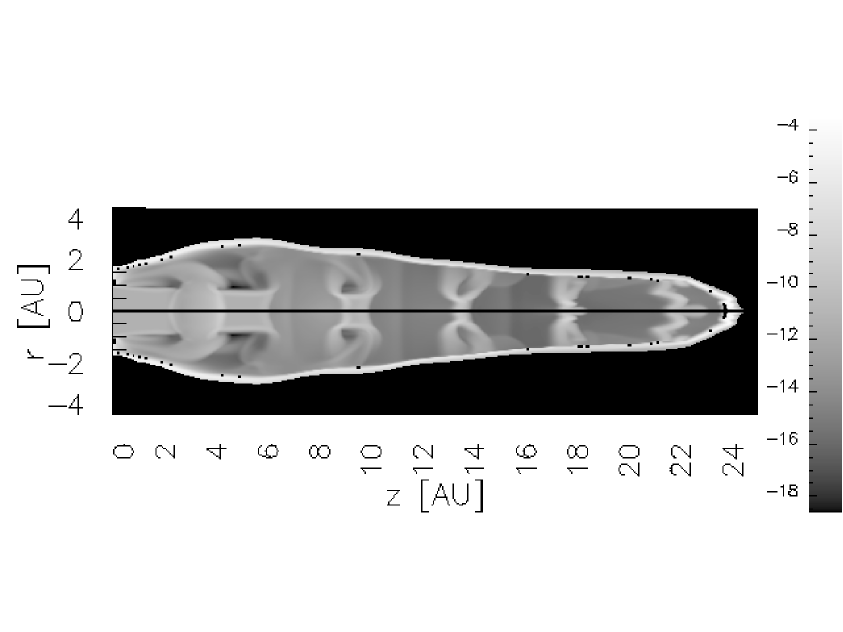
Figure 14: Logarithm of Bremsstrahlung emission of the model i with cooling in $\rm{erg\,s}^{-1}\rm{cm}^{-3}$; the shocked ambient medium collapsed, therefore the emission features of the jet beam are visible in the whole jet width

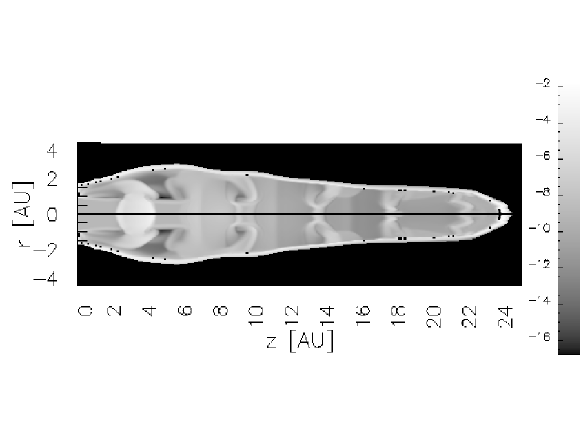
Figure 15: Logarithm of Synchrotron emission of the model i with cooling in $\rm{erg\,s}^{-1}\rm{cm}^{-3}$

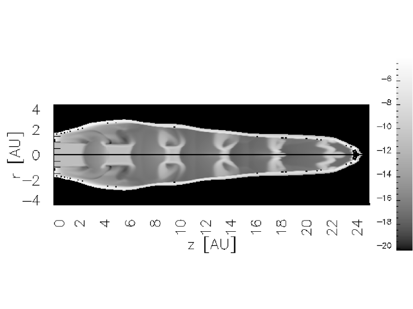
Figure 16: Logarithm of H i line emission of the model i with cooling in $\rm{erg\,s}^{-1}\rm{cm}^{-3}$

The integrated luminosities at day 74 are:

$$L_{\rm{Bremsstrahlung}} = 1.15\cdot 10^{33}\,\rm{erg\,s}^{-1}$$

$$L_{\rm{HI}} = 6.96\cdot 10^{32}\,\rm{erg\,s}^{-1}$$

The integrated synchrotron emission was omitted because it is only a relative and qualitative presentation. $L_{\rm{HI}}$ accounts only for the H i recombination emission. The total cooling emission in all emission lines is certainly higher. Thus the dominant cooling radiation should be atomic emission lines.

For the comparison of the emission plot with observations it should be considered that the H i plot would not be representative for all optical lines. For example emission from collisionally excited lines like Ca ii is only expected from the very coolest $T<15000$ K regions in the jet knots. No emission would come from the hot jet beam or the cocoon because there Ca would be in a higher ionization state than $\@element[+]{\mathrm{Ca}}$. Thus the knot structure may be particularly well defined in such low ionization lines. Similar selection effects must be considered for the observations of the Bremsstrahlung radiation. Thermal free-free radiation in the radio range would strongly favor the low temperature emission regions, such as the dense knots, while the Bremsstrahlung radiation observable with X-ray telescope would only originate from the very hottest, low density regions in the hot beam or the cocoon. The plot for the Bremsstrahlung simply includes the emitted radiation in all wavelength bands.

Figure 17: Evolution of the kinetic, bremsstrahlung and H i luminosity

Fig. 17 shows the evolution of the kinetic, bremsstrahlung and H i luminosity until day 74. The emitted luminosity is about 50 per cent of the kinetic luminosity. The peaks in the emitted luminosity coincide with the merging of the pulses with the bow shock (see Fig. 13). These “flashes” are in accordance with simple analytical models (Raga & Cant$\acute{\textrm{o}}$ 2003).

5 Calculations of jet absorption profiles

Using the model results from the hydrodynamical simulations, we calculate the absorption line structure.

As emission region we define a disc in the equatorial plane ($z=0$) which extends to a radius $r_{\rm em}$. For each grid cell inside this region, we assume a normalized continuum emission and a Gaussian emission line profile:

$$I_{0}=1+I_{\rm peak}\cdot\exp{\left(-v^{2}/\sigma^{2}\right)}.$$ (9)

This initial intensity is taken to be independent of position $r<r_{\rm em}$.

Further we consider the possibility of different system inclinations $i$ for the calculation of light rays from the emission region through the computational domain. We consider only absorption along straight lines and neglect possible emissivity or scattering inside the jet region.

The initial continuum and line emission (9) is taken as input for the innermost grid cell of each path. We then calculate the absorption within each grid cell $j$ along the line of sight according to:

$$I_{j} = I_{j-1}\cdot e^{-\tau_{\lambda}}$$

$$\tau_{\lambda} = \frac{\pi\,e^{2}}{m_{e}\,c}\,\lambda_{kl}\,\left(1-\frac{v_{j}}{c}\right)\,\frac{\rho_{j}\,\eta}{m_{H}}\,\Delta x_{j}\,f_{kl}$$ (10)

$$= \mathcal{C}_{kl}\,\Delta x_{j}\,\mathcal{F}(v_{j},\rho_{j})\,,$$

where $e$ is the electron charge, $m_{e}$ the electron mass, $c$ the speed of light, $\lambda_{kl}$ the rest frame wavelength of the transition, $m_{H}$ the proton mass and $f_{kl}$ the oscillator strength. The parameters are constant for a given atomic transition. $\Delta x_{j}$ is the length of the path through grid cell $j$ which is a function of the inclination $i$.

The parameters depending on the different hydrodynamical models are the velocity projected onto the line of sight $v_{j}$, the mass density $\rho_{j}$ and $\eta$ the relative number density with respect to hydrogen $\eta=n_{k}/n_{\rm H}$ of the absorbing atom in the lower level $k$ of the investigated line transition. The velocity is binned for the calculation of the absorption. The size of the bins $\Delta v$ can be interpreted as a measure of the kinetic motion and turbulence in one grid cell. This absorption dispersion helps to smooth the effects of the limited spatial resolution of the numerical models.

The absorption calculation through the jet region is repeated for all possible light paths from the emission region to the observer. The arithmetic mean of the individual absorption line profiles from all path is then taken as resulting spectrum.

5.1 Model parameters

The quantities determining the absorption line profiles are first the parameters defining the hydrodynamical model. These are for our model grid the pulse velocity, the pulse density, and the time (day) in the simulation. For model i we have to distinguish further between adiabatic calculation and calculations including radiative cooling.

For the emission from the jet source, the size of the emission region $r_{\rm em}$ must be fixed. For the emission spectrum we adopt throughout this paper a normalized continuum and an emission line component at rest velocity (the same transition as the calculated jet absorption line) with $I_{\rm peak}=6$, $\sigma=100$ km s^-1. An additional parameter is the inclination $i$ under which the system is seen.

The parameters of the absorbing transition are defined by the rest wavelength $\lambda_{kl}$, the oscillator strength $f_{kl}$ and the population of the absorbing atomic level $\eta=n_{k}/n_{\rm H}$. Further we have to define the velocity bin size $\Delta v$ which is a measure for the adopted turbulent (and kinetic) motion of the absorbers.

5.2 Results for different model parameters

The structure of the synthetic absorption profiles reflect in some way the hydrodynamical structure of the jet outflow. The hydrodynamical variables determining the absorption profile are the density and the velocity projected on to the line of sight. The density, the velocity component parallel and the velocity component perpendicular to the jet axis are plotted in Fig. 18 for the model with radiative cooling at day 74. While the adiabatic jet produces a very extended and highly structured jet cocoon, the model i with radiative cooling produces an almost “naked” jet beam with practically no jet cocoon, but with a well defined and sharp transition towards the ambient medium.

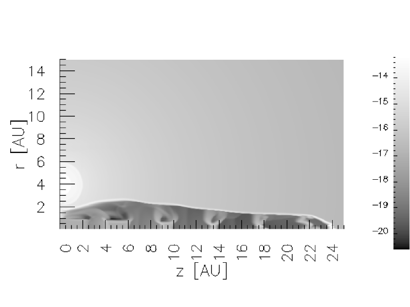
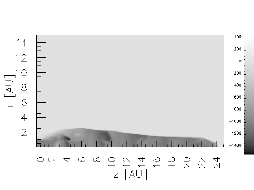
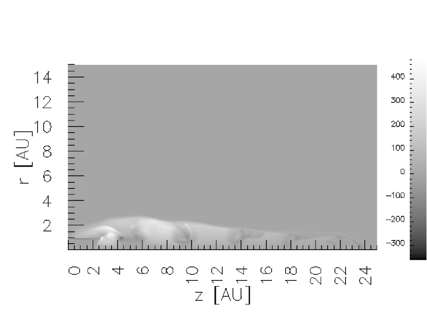
Figure 18: Pulsed jet model i with radiative cooling at day 74: Grey scale plots of the logarithm of density in g cm^-3 (top), of the velocity components parallel (middle) and perpendicular (bottom) to the jet axis in km s^-1

In the adiabatic model four different velocity regions can be distinguished (Fig. 19):

• the jet beam with high outflow velocities of $-800$ to $-1400$ km s^-1,

• the cocoon and bow shock region with velocities of $-10$ to $-800$ km s^-1,

• the external medium, the companion star and its wind with velocities around 0 km s^-1, and

• the backflow near and besides the jet head with velocities of 0 to $+500$ km s^-1.

In the jet models with radiative cooling there exists neither an extended cocoon and bow-shock region nor a backflow region. These regions are suppressed into a narrow transition region between jet beam and external medium due to the high density and the efficient cooling. Thus the model with cooling has essentially only two velocity regions:

• the jet beam, and

• the external medium.

5.3 Synthetic absorption line profiles

From our model simulations we can calculate from the density and velocity structure of the jet (e.g. Fig. 18) the synthetic absorption line profile for different line of sights.

For the emission region we assumed that it has an radius of $r_{\rm em}=1$ AU and the resulting spectrum is the mean of the corresponding line of sights distributed over this emission area. For the atomic transition we use the parameters $\lambda_{kl}=3934$ Å, $f_{kl}=0.69$ and $\eta=2\cdot 10^{-6}$ appropriate for the Ca ii K transition. For $\eta$ we just assumed that all Ca-atoms are in the ground state of $\@element[+]{\mathrm{Ca}}$. This is useful for the investigation of the expected absorption line structures introduced by the different velocity regions. However, the gas temperature in the adiabatic models is far too high to have Ca in the form of $\@element[+]{\mathrm{Ca}}$. This will be discussed in Sect. 5.6. The velocity bin width for the calculation of the absorption profiles is set to $\Delta v=10$ km s^-1. The parameters for the emission line component in the initial spectrum are $I_{\rm peak}=6$ and $\sigma=100$ km s^-1.

Figure 19: Four different absorption regions in the adiabatic model i caused by the jet beam, the bow shock region, the external medium and the backflow; in model i with cooling only the jet beam and the external medium are clearly visible, while the bow shock region creates only a slight absorption and no backflow is present

Figure 19 shows the resulting synthetic absorption line profiles calculated for the model i without cooling (adiabatic model) and with cooling.

The model with cooling shows a strong, broad absorption from the velocity region I centered around RV $=-1100$ km^-1 from the jet beam. In addition there is a saturated, narrow absorption component in the middle of the emission component caused by the almost stationary stellar wind of the cool giant (velocity region III) in front of the jet bow shock.

The absorption spectrum of the adiabatic model i is much more structured. Besides the velocity component I and III from the jet beam and the ambient medium respectively, there is also a broad velocity component from the bow shock region in the velocity range $v=-400$ to $+100$ km s^-1. This component can be associated with the RV-region II of the jet cocoon. The line of sight goes for this geometry not through the extended backflow region of the adiabatic jet. Signatures of the backflow regions may be visible for other line of sight geometries.

Surprisingly, the structure of the main absorption trough is quite similar in both the adiabatic model and the model with radiative cooling.

5.4 Different line of sight geometries

In this section we describe the dependence of the jet absorption structure on the line of sight inclination and the emission region size for the jet with radiative cooling.

In Fig. 20 the synthetic absorption profiles are given for different radii $r_{\rm em}=1,2,3$ AU of the disk-like emission region. The system inclination is set to $i=0^{\circ}$, therefore the projected velocity is equal to the velocity component parallel to the jet axis.

For $r_{\rm em}=1$ AU the gas inside the jet beam (region I) with $v=-800$ to $-1300$ km s^-1 produces absorptions. The external medium (III), in front of the bow shock, absorbs the peak of the emission line. For higher values of $r_{\rm em}$ no additional structure appears, but the high velocity component is averaged out and therefore less strong.

Figure 20: Synthetic absorption line profile for three different radii $r_{\rm em}=1,2,3$ AU of the emission region. Calculations for model i with cooling (Fig. 18) and inclination $i=0^{\circ}$. The appearance of absorption component created in the jet beam and averaging effects are detectable

Figure 21: Synthetic absorption line profile for the model i with cooling seen under the inclination $i=0^{\circ}$, 3^∘ and 6^∘. The radius of the emission region is $r_{\rm em}=1$ AU. The splitting of the main absorption component into two distinct components with increasing system inclinations is visible.

The absorption line structure depends also on the system inclination as shown in Fig. 21. In this figure the synthetic spectra are compared for the inclinations $i=0^{\circ},3^{\circ}$ and $6^{\circ}$ for an emission region of radius $r_{\rm em}=1$ AU. For $i=3^{\circ}$ and $i=6^{\circ}$ the absorption components are redistributed in comparison to the $i=0^{\circ}$-case, because then other regions are along the line of sight while regions in the jet beam at large $z$ are missed. A region of weakened absorption appears and splits the main absorption component into two distinct components.

5.5 The velocity bin size

The velocity structure in the synthetic jet absorption profile represents an average of the jet which is limited by the spatial resolution. The real velocity structure inside one grid cell is certainly more complex, mainly due to turbulent small scale gas motions. Therefore the discrete velocity value for the absorption of one grid cell should be replaced by a velocity dispersion. The strength of this dispersion, however, is not known. Thermal motion in our temperature regime leads to values of about 10 km s^-1, turbulence can increase them to 50 km s^-1 and more. The effect of such a velocity dispersion can be considered in the calculation of the absorption line by the binning of the velocities into broader bins. For broader velocity bins, simulating a larger velocity dispersion of the absorbing atoms, a smoother jet absorption profile with less structure is obtained as shown in Fig. 22. The observations show typically a smooth absorption line structure indicating a significant velocity turbulence.

Figure 22: Theoretical absorption line profile for values of the velocity bin size $\Delta v$ (10, 20, 40, 80 km s^-1); higher velocity dispersions lead to higher equivalent widths and smoother spectral absorption structures.

5.6 The ionization problem

In all the jet absorption profile calculations in the previous sections we have assumed that all Ca atoms are singly ionized.

In the adiabatic models the gas temperature is far too high for $\@element[+]{\mathrm{Ca}}$-ions. Assuming collisional ionization equilibrium, $\@element[+]{\mathrm{Ca}}$ would be the dominant ionization stage for $T_{e}<15000$ K. The relative abundance $\@element[+]{\mathrm{Ca}}$/Ca is less than 1 % for $T_{e}>25000$ K or less than 0.01 % for $T_{e}>250000$ K. After fitting the ionization balances from Sutherland & Dopita (1993) with

$$\eta(T)=\eta(0)\,\frac{1}{\exp(T/1000-14)+1}$$ (11)

and introducing this into the calculation, for our adiabatic model no absorption is present if ionization equilibrium is considered for the $\@element[+]{\mathrm{Ca}}$ abundance.

Even in the model with cooling, the jet gas temperature is slightly too high to produce a strong Ca ii absorption (Fig. 23). The absorption generated by material which is cooler than 10⁵ K is of the order of 60 % in the model with cooling, the material with temperatues below $3\times 10^{4}$ K is responsible for 48 % of the absorption. Therefore the temperature in our model with cooling is only slightly overestimated.

Figure 23: Theoretical absorption line profile with and without a temperature dependent $\eta$ for the model i with cooling (day 65)

The high temperature of the model jet gas, compared to the observations, could be explained by unsufficient cooling. As the cooling is proportional to the density squared, higher density gas in the jet model would cool faster and down to the required temperature to account for the observed Ca ii absorption. This may be achieved with models having higher gas densities in the jet or pulse. Another possibility is, that high density clumps may form, for which the cooling would be very efficient. However, the spatial resolution of our model grid is too coarse for simulating such small scale structures. A third reason could be the choice of the used cooling curves. They extend only down to temperatures of $10^{4}$ K. Below that value, no cooling is achieved in the present treatment. The adding of more cooling processes could improve the models and perhaps also solve the ionization problem.

6 Time variability

As next step the temporal evolution of the highest velocity component is investigated. This “edge” velocity for the variable absorption originates from the most recent pulse, close to the jet nozzle, which is not yet slowed down as much as the previous pulses. As this gas is located close to the continuum emission region, the corresponding absorption feature is present for all viewing angles considered and essentially independently from the size of the emission region.

In Fig. 24, the maximum outflow (negative) velocity of the high velocity component is plotted between day 360 and 380 for the first four adiabatic models and between day 50 and 74 for the one with cooling.

Figure 24: Time variability of the high (negative) velocity component for models i-v (top) and for model i with cooling (bottom)

The first result is the fact, that pulses without velocity enhancements (only density changes) as investigated in the four adiabatic models v to viii, produce hardly any velocity effects. The velocity variations created by interactions between different density regions in the jet are only of the order of a few 10 km s^-1 and only in the model v, where the density in the pulse is the smallest. It seems unlikely that high velocity components can be produced by density jumps in the jet outflow.

The simulations with high velocity pulses show all a qualitatively similar behavior, with a sudden outflow (negative) velocity increase to the pulse velocity of $-2000$ km/s followed by a velocity decay during the following days. Closer inspection of the evolution of the high velocity component shows some differences between the four adiabatic models i – iv to the model i with cooling. In the latter, the velocity drops within one or two days from the initial –2000 km s^-1 to –1400 km s^-1 and then much slower — apparently asymptotically — to a stationary value of –1300 km s^-1 during the next four days. In the adiabatic model i, the first drop is similar, but the slow decay seems to be only a plateau of two days, after that the velocity drops to –1150 km s^-1. The model ii shows the same behavior but with higher velocities (–1400 and –1250 km s^-1). The last two models iii and iv decay again in an asymptotic manner to –1300 km s^-1 and –1550 km s^-1, respectively.

The fact, that the structure and time variability of the high velocity components are quite similar in the adiabatic models and the model with radiative cooling, shows that also the former have their merits. As their computational requirements are by far smaller than those for models with radiative cooling, they can be used for (additional) parameter studies without a great loss of accuracy. Another point of future investigation could be then the influence of different jet pulse shapes and frequencies on the structure of the high velocity components.

7 Jet absorption variability: comparison with observations

Based on our simulations of jet pulses we construct now sequences of absorption line profiles which can be compared to the spectroscopic observations of the MWC 560 jet outflow. For the line of sight we adopt a direction parallel to the jet (inclination $i=0^{\circ}$) and an emission region size of $r_{\rm em}=1$ AU. Atomic parameters are taken for the Ca ii absorption as in previous sections.

7.1 Variations of the jet absorption for adiabatic models

For the comparison with the observations we consider only the adiabatic models i - iv. One can directly see that the adiabatic models v - viii can be discarded because they do not show high velocity components in the synthetic absorption line profiles (Fig. 24, middle). For the models i to iv the density in the jet pulses increases from 0.25, 0.5, 1 to 2 times the interpulse jet density at the nozzle.

A major discrepancy in the jet absorption between our adiabatic simulations and the observations is seen in the velocity region between $-300-0$ km s^-1 where the calculated absorption is grossly overestimated.

This feature appears whenever the light path from the emission region to the observer travels through the jet head (bow shock-Mach disk) region (Fig. 25). The simulations were stopped when the jet reached the opposite boundary. At this position, the density of the external medium has dropped to the density value of the jet at its nozzle. In reality, the jet would extend further into a region where the density of the external medium is by far smaller. Then the densities in the jet head region also should be smaller and therefore the depth of the absorption. To account for this, we disregard the absorption produced in this region. Thus the calculations of the absorption line profile is only done for the line of sight from $z=0$ AU to 40 AU in model i and iv and 37.5 AU in model ii and iii.

Figure 25: Theoretical absorption line profile of the adiabatic model i for values of $z_{\rm max}$; the absorption feature at RV $\approx$ -300 km s^-1 is produced by the bow shock-Mach disk region

Potentially the adiabatic models may show absorptions with RV $>0\,{\rm km}\,{\rm s}^{-1}$ and some synthetic spectra show weak traces of an absorption at the base of the red wing of the emission line. It must be noted that the chosen line of sight geometry for the synthetic absorption profiles avoids the jet backflow region. The backflow region would be clearly visible for inclined line of sights or more extended emission regions.

Further we disregard in the line profile calculation the ionization problem discussed in section 5.6 assuming that all Ca-atoms are singly ionized $\@element[+]{\mathrm{Ca}}$. This is questionable particularly for the adiabatic jet models.

With these restrictions we obtain in the simulations absorption line profiles which are shown in Fig. 26. There, sequences of the synthetical absorption line profiles are plotted for eight consecutive days for the adiabatic models i–iv.

There exists quite some agreement between the synthetic profiles and the observations. The simulations produce the detached, broad absorption component as observed for times where no new high velocity component was ejected during the previous days in the jet nozzle.

Not well reproduced is the strength of the high velocity absorption components due to the jet pulses. They are too weak by a substantial amount. At least one can see that the equivalent width and the depth of the high velocity components increases as the density in the jet pulse increases from $n_{\rm pulse}=1.25,2.5,5$ to $10\times 10^{6}\,{\rm cm}^{-3}$ for models i, ii, iii and iv respectively. Further it is visible, that the high velocity absorption components of the higher density pulses require a longer time scale to be decelerated than the low density pulses. For example in Fig. 26 (top), these components can be detected in only two consecutive days while they are present during three days in Fig. 26 (middle).

Figure 26: Sequence of absorption line profiles for eight consecutive days of model i (top), model iv (middle) and model i with cooling (bottom)

Also a shallow component between the absorption trough and the emission line is visible in all models. The absorption is stronger for the adiabatic jets with higher pulse densities. The strength of this absorption is anticorrelated with respect to the high velocity component as in the observations.

7.2 Variations of the jet absorptions for the model with cooling

Also for calculations of the jet absorptions from model i with cooling we have excluded the line of sight section through the ambient medium in front of the jet. This avoids the narrow, saturated absorption component in the emission component. Thus the calculation of the absorption profile was only performed from $z=0$ to 21 AU.

The absorption for the jet model i with cooling behaves qualitatively similar to the adiabatic model. There is a broad jet absorption trough centered at about $\approx$ -1100 km s^-1, which is completely detached from the emission component. And again the high velocity absorptions are far too weak when compared with the observations. Comparing the models i with and without cooling seems to indicate, however, that they are a bit deeper and persist for a somewhat longer time in the model with cooling.

We like to note that it was also assumed for model i with cooling that all Ca is singly ionized. According the the model calculation the jet gas would be too high for $\@element[+]{\mathrm{Ca}}$, but the discrepancy between required temperature for $\@element[+]{\mathrm{Ca}}$ and calculated temperature is not very large, in particular much smaller than for the adiabatic case.

8 Summary and discussion

This paper describes pulsed jet models for parameters representative for symbiotic systems. Two main types of simulations were performed, a small model grid for adiabatic jets with different jet pulse parameters and one simulation including radiative cooling.

For the adiabatic jet models some quantitative differences are present for the different pulse parameters, but qualitatively the model results are very similar.

Huge differences can, however, be seen between the adiabatic models and the model which includes radiative cooling. Compared to the adiabatic models the most important effects induced by radiative cooling are:

• The energy loss through radiation lowers the pressure and the temperature which leads to a much smaller radial extension of the jet, so that the cross section and the resistance exerted by the external medium is strongly reduced leading to a significantly higher bow shock velocity.

• The internal structure of the pulsed jet with cooling shows a well defined periodic shock structure with high density, low temperature knots separated by hot, low density beam sections. Contrary to this in the adiabatic jet the hottest regions have the highest densities while the density is low in cool regions. The temperature and density contrast is much more pronounced in the models with cooling.

These differences are generic for model results from jet simulations without and with cooling. For the particular model i described here we can now quantify these differences.

• The jet radii are 10 AU for the adiabatic jet and 2.5 for the jet with cooling. These values are determined for model jets with the same axial length of 24 AU.

• The bow shock velocity after 74 days is about $200\,{\rm km}\,{\rm s}^{-1}$ in the adiabatic model compared to $730\,{\rm km}\,{\rm s}^{-1}$ in the cooled jet.

• The gas temperature in the adiabatic jet is everywhere (except for the initial jet gas in the nozzle) higher than $T\approx 2\cdot 10^{5}$ K and goes up to $T\approx 10^{7}$ K in the high density shock regions. In the jet model with cooling the temperature is really low $T\approx 10^{4}$ K in the cool, high density knots. The hot beam regions are $T\gg 2\cdot 10^{5}$ K.

• The density contrast between cool and hot regions is about a factor of 30 in the adiabatic jet, but a factor of 1000 in the jet with radiative cooling. Note that high density regions are hot in adiabatic models, while they are cool in the models with cooling.

These huge differences show clearly that adiabatic jet models are far from reality if radiative cooling is indeed important. Therefore jet models with radiative cooling should be investigated in much more detail for the high jet gas densities encountered in symbiotic systems.

Unfortunately, the time scales of cooling processes are several orders of magnitude shorter than those of hydrodynamical ones. This is a large numerical problem which is demanding high computational costs. But as mentioned above, these costs are necessary to get new insights into the physics of jets in symbiotic stars.

Until now, only two-dimensional simulations have been performed, also due to high computational costs and memory demands of 3D-simulations. In those simulations, the red giant would be taken into account correctly, not as a ring, and its influences on the jet, the gravitation and the stellar wind, would not be symmetric anymore. This would result in the backflow being blocked only in a small segment, therefore the adiabatic jet should be more turbulent from the beginning.

As Kössl & Müller (1988) and Krause & Camenzind (2001) have shown in their simulations, the numerical resolution determines, if one sees the transition from the laminar to the turbulent phase or not. Also in our simulations, this transition can be seen, implying that the resolution here is not too small. An increased resolution should not change the main result, the shrinking of the cocoon and the necessity of performing hydrodynamical simulations with cooling to understand the structure and emission of jets in symbiotic stars.

8.1 Comparison with symbiotic systems

Our model calculations make various predictions for jets in symbiotic systems. We focus here on the basic question whether the observations of symbiotic systems support more the adiabatic jet model or the jet model with cooling.

For MWC 560 the spectroscopic observations show strong absorptions from low ionization species such as Ca ii, Fe ii and Na i. Absorptions from neutral or singly ionized metals are only expected for cool gas with temperatures around $T\approx 10000$ K or lower. The strength of these absorptions suggest that a substantial fraction of the jet gas must be in this cool state as in the jet model with cooling. This is incompatible with the hot gas temperatures $T\gg 10^{5}$ present in adiabatic models. The presented adiabatic jet models are not able to produce low temperature regions.

The propagation of the jet bow shock was well observed for the outburst in CH Cyg. The jet expansion was linear and fast $\approx 1500\,{\rm km}\,{\rm s}^{-1}$ producing after one year a narrow jet structure with an extention well beyond 300 AU. The estimated jet gas temperature was found to be below 10000 K. This is again in very good agreement with the jet model with cooling. According to our models an adiabatic model is expected to produce a jet with a lower expansion velocity, a broader jet beam emission and most importantly only high temperature jet gas. For CH Cyg it must be said that the initial jet conditions “at the nozzle” are not known.

Less clear is the situation in R Aqr. Although jet features can be traced down to a distance of less than 20 AU, it is not clear whether the jet gas is cool or hot. A proper motion for the emission features in the range 36 to 240 km s^-1 has been derived. This would be more in the range of the gas motion of the adiabatic models. However it is not clear from where the observed emission originates, from the jet gas or the surrounding gas excited by shocks induced by the jet propagation. The small jet opening angle of 15^∘ favors more a jet with cooling, but a strong disk wind or a steep density gradient for the circumstellar gas may also help to enhance the collimation of an adiabatic jet.

Thus, the comparison between model simulation and observations suggest strongly that radiative cooling is important for jets in symbiotic systems. The fact, that the model with cooling describes the observations better than those without cooling, means that the cooling time scale in the jet of symbiotic systems must be shorter than the propagation time scale (i.e. expansion time scale of the adiabatic gas) which is of the order of hundred days. This condition sets a lower limit for the density inside the jet of about $n\approx 10^{6}\leavevmode\nobreak\ {\rm cm}^{3}$ ( $T\approx 10^{4}$ K ) which is consistent with our initial parameters.

8.2 The synthetical absorption line profiles

Synthetic line absorption profiles are presented in this work, based on hydrodynamical calculations of pulsed jets. These “theoretical” profiles are compared to observations of the jet in the symbiotic system MWC 560.

An important point is that the gas temperature in the adiabatic jet is everywhere far too high to produce the low ionization absorptions seen in the observations. Even in the model simulations including radiative cooling the gas temperature in the jet is too high for producing the observed Ca ii line strengths. Thus, more efficient cooling of the jet gas is required. This can be achieved with higher gas densities in the model jet outflow or perhaps with higher resolution of the hydrodynamical calculation, which may then be able to resolve high density small scale clumps. A third solution could be the adding of further cooling processes which would be important at temperatures below $10^{4}$ K. Additional modeling is required to investigate which of these solutions is more likely.

Disregarding the ionization problem, we calculated the synthetic jet absorption line structure. This line structure represents essentially a projection of the gas radial velocity along the line of sight, which is more or less parallel to the jet.

A success of our computations is that the basic structure of the jet absorption in MWC 560, which is the broad, detached component, can be well reproduced. The mean velocity and the velocity width is in good agreement with the observations. Surprisingly, both adiabatic jet models and the model with cooling provide qualitatively similar absorption profiles for the jet beam and the transient high velocity components. Here are the merits of the adiabatic models which enable us to perform parameter studies which would be highly expensive for models with radiative cooling. However, as we disregard the ionization equilibrium we should more correctly speak of the projected RV distribution of the gas.

Also the temporal evolution of the highest velocity components of the transient jet pulses follows the observed behavior. Not well reproduced by our simulations are the strengths of the high velocity components. They are far too week in our simulations. This suggests that higher gas densities are required for the jet pulses.

From the presented comparison between the synthetic and observed jet absorption line structure we conclude that the general direction of our modeling is correct. Due to the high temperature the adiabatic simulations are inadequate to explain the observed low ionization absorptions observed. However, disregarding the temperature, they provide an easy to calculate mean to explore the projected velocity distribution of the gas in a pulsed jet along the line of sight. Our current jet simulation with radiative cooling solves the ionization problem not fully, as the gas temperature is still somewhat too high. However, the discrepancy is rather small and may be solved with calculations having higher gas densities in the jet in order to enhance the efficiency of gas cooling. Higher gas densities are also required for the strengths of the absorption in the transient high velocity components.

With our comparison between synthetic and observed line profiles we have demonstrated the huge diagnostic potential of the spectroscopic observations of the jet absorption profiles in MWC 560. The information, which can be extracted from these observations, is unique for astrophysical jets and is therefore a most important source for a better understanding of astrophysical jets, in particular for the detailed investigation of the propagation and evolution of small scale structures originating in the jet acceleration region.

The shape of the high velocity components is in all simulations discrete. This could be a result of the assumed rectangular velocity and density steps for the pulses. A Gaussian form possibly could smooth the components in the absorption line profiles.

A point where these simulations can be further improved is the elapsed time and therefore the calculated length of the resulting jet. We only simulated the jet until it reached a length of 50 AU. At this point, however, the density of the environment has decreased to the density in the jet nozzle. A transition of the initially underdense jet ($n_{\rm jet}/n_{\rm wind}<$ 1) towards an overdense jet will occur, which should result in changed kinematics. A direct effect on the absorption line profiles should be a decreased density of the shocked ambient medium, which was artificially cut out in the calculation of the profiles in this paper. After extending the computational domain, this manipulation should not be necessary. Simulations with larger domains are currently being carried out.