A photometrically and kinematically distinct core in the Sextans dwarf spheroidal galaxy

Abstract

We present the line of sight radial velocity dispersion profile of the Sextans dwarf spheroidal galaxy (dSph), based on a sample of 88 stars extending to about $1^{\circ}$ ($\sim 1.5$kpc). Like the Draco and Ursa Minor dSphs, Sextans shows some evidence of a fall-off in the velocity dispersion at large projected radii, with significance $p=0.96$. Surprisingly, the dispersion at the very centre of Sextans is close to zero (with significance $p=0.96$). We present evidence which suggests that this latter change in the stellar kinematics coincides with changes in the stellar populations within the dSph. We discuss possible scenarios which could lead to a kinematically and photometrically distinct population at the centre of Sextans.

1 Introduction

It has long been known that the velocity dispersions of Local Group dwarf spheroidals (dSphs) imply mass-to-light ratios $M/L$ of up to $\sim 100\,M_{\odot}/{\rm L}_{\rm\odot}$. Until recently, all estimates of dSph $M/L$ have been based upon a measurement of the central velocity dispersion, and the assumption of mass follows light. The advent of datasets of hundreds of discrete radial velocities of bright stars in the nearby dSphs has changed all this. To date, the line-of-sight velocity dispersion profiles in the Fornax, Draco and Ursa Minor dSphs have been mapped out right to the optical edge (Mateo, 1997; Kleyna et al., 2002; Wilkinson et al., 2004).

In this paper we turn our attention to the Sextans dSph and present the first results from our new radial velocity survey. The new data show an almost flat velocity dispersion to large radii, with some evidence of a fall-off in the outer parts similar to that seen in Draco and Ursa Minor (Wilkinson et al., 2004). Surprisingly, Sextans appears to be kinematically cold at the very centre. This is the second localised cold population observed in a dSph (Kleyna et al., 2002), and it coincides with observable changes in the composition of the stellar population. We suggest that the nucleus of the Sextans dSph contains a dynamically separate component, possibly the remains of a star cluster dragged to the centre by dynamical friction.

2 OBSERVATIONS

2.1 Velocities

We observed Sextans with the multifibre instrument AF2/WYFFOS on the William Herschel Telescope on La Palma on 11-16 March 2004. Approximately two of these six nights were lost to weather or technical problems. We reduced the spectra using a modified version of the IRAF WYFRED task, and we obtained the final velocities using the FXCOR cross-correlation function (CCF) velocity package. From the point of view of the data reduction, Sextans presents particularly thorny difficulties. Due to the bulk line of sight velocity of Sextans, all three Ca triplet lines absorption lines used to measure the velocity are embedded in bright sky emission lines. Hence it is of paramount importance to subtract the sky spectrum accurately, and to distinguish between those correlation peaks caused by stellar absorption lines and those arising from a random or systematic sky residual.

Each WYFFOS pointing consisted of approximately 75 fibres allocated to objects, and an average of 27 sky fibres interleaved among the object fibres. After rebinning each spectrum to a common linear dispersion and flattening with a tungsten lamp spectrum, we constructed a sky spectrum for each object fibre by median-combining the five sky spectra closest to the object spectrum on the CCD, thereby minimising the effects of dispersion-direction PSF variations. Next, we subtracted the sky spectra from the object spectra by modelling each spectrum as the sum of a third-order polynomial plus a multiple of the sky, and minimising the integrated absolute deviation of the model from the actual spectrum, excluding those regions known to contain stellar absorption lines. Effectively, this procedure subtracts out the correct amount of sky by minimising the sky line residuals. As the final step before computing velocities, we shifted each spectrum to a common heliocentric velocity frame.

For our previous work on Draco and UMi (Kleyna et al., 2001, 2002, 2003; Wilkinson et al., 2004), the sky lines were safely separated from the stellar lines, and it was possible to combine all of the good spectra for an object into a single spectrum, producing an unambiguous CCF against a synthetic template. With Sextans, it was difficult to distinguish good spectra from bad, so we elected to obtain as many individual measurements as possible by measuring a velocity with each of the three Ca triplet lines in each one hour exposure, using FXCOR in an automated mode, and allowing it to select the highest CCF peak between -200 and +400 $\;{\rm km\,s}^{-1}$. For each velocity, FXCOR also gives an uncertainty $\propto(1+R)^{-1}$, where $R$ is the Tonry-Davis $R$ value (Tonry & Davis, 1979).

Next, we constructed the following sigma-clipping procedure: for a set of measured velocities and their nominal uncertainties $\sigma_{i}$, we compute the median of the set, discard the farthest outlier (in terms of $\sigma_{i}$), and iterate until all of the remaining points are less than 2.5 $\sigma_{i}$ from the median. Then we computed the velocity of each object in each of lines 1, 2, and 3 by applying the sigma clipping procedure to all measurements in the line in question. We observed that the velocities in line 2 and 3 were consistent, but generally disagreed with line 1 – this is not surprising, as line 1 is the weakest line, and is atop the strongest sky line. Thus we elected to compute our final best velocity for each object by applying the sigma clipping procedure to the combined set of velocities from lines 2 and 3.

To accept a velocity for our subsequent analysis, we required that there exist at least four velocities, representing at least $2/3$ of the inputs, which survive the sigma clipping procedure. In all, 88 Sextans member stars from the combined $2+3$ lines within 30 $\;{\rm km\,s}^{-1}$ of the dSph’s median velocity met these criteria.

Our sigma clipping and subsequent error estimates depended on the validity of the $R$-value velocity uncertainties produced by FXCOR. Each final velocity, as a Gaussian-weighted average of individual velocities, had an associated $\chi^{2}$. The mean $\chi^{2}$ per degree of freedom for all member and non-member stars with good velocities was 0.93, suggesting that the FXCOR velocities were indeed valid. Repeating the clipping procedure after rescaling the FXCOR errors by 0.75 and 1.33 produced a $\chi^{2}$ per degree of freedom that deviated from the expected value of 1 in the expected directions. The smallest $P(\chi^{2})$ observed for a Sextans member was 0.004, which would be expected to occur by chance in a sample of this size a third of the time.

Figure 1: Distribution of pseudo-velocities of sky fibres when processed as though they were data fibres, for each of the three lines of the Ca triplet. Lines 1 and 2 produce a spurious peak near the mean velocity of Sextans, resulting from random and possibly systematic sky residuals. Line 3, on the other hand, produces a relatively unbiased distribution of spurious velocities.

Despite our care to sift out spurious velocities from our data, the sky line contamination remains a concern. Fig. 1 shows the result of reducing our sky fibres as though they were object fibres. Because lines 1 and 2 of the Ca triplet are directly under two strong sky lines, the residue of the sky tends to produce spurious velocities at 233 and 223 $\;{\rm km\,s}^{-1}$, respectively. The peaks actually becomes stronger if we limit ourselves to larger Tonry-Davis $R$ values, probably because we are picking out spectra with systematic sky subtraction problems. Only line 3, embedded in a dense cluster of lower amplitude sky lines, shows an unbiased distribution of spurious velocities. Because of this potential source of contamination, we will take care to verify any observed kinematical qualities of Sextans using line 3 alone, as well as with our best $2+3$ velocities.

Figure 2: Individual velocities as a function of projected radius $R$ for the combined data (using lines 2 and 3 of the Ca triplet), and for lines 1, 2, and 3 individually. Outer dotted lines show our membership limits, and the inner dotted line is the median of the entire data set.

Fig. 2 shows our individual velocities as a function of projected radial distance. The data using only line 1 are obviously of much poorer quality than for lines 2 and 3; in particular, the median velocity for line 1 is $232.5\,\;{\rm km\,s}^{-1}$, whereas the medians for lines 2 and 3 are 226.6 and 225.3 $\;{\rm km\,s}^{-1}$, respectively. Immediately apparent to the naked eye is the apparent tendency of the outermost stars of the top $2+3$ panel to cluster very tightly around Sextans’ mean velocity; this kinematic coldness at large $R$ was also found to be present in UMi and possibly Draco (Wilkinson et al., 2004). Unfortunately, the data for lines 2 and 3 alone are not of sufficiently good quality to support this conclusion on their own.

2.2 Comparison with previous work

In the past, repeated velocity measurements of individual Sextans stars have been inconsistent from observer to observer, probably because of the severe sky contamination. Suntzeff et al. (1993), (henceforth S93), measured 43 velocities in Sextans using the Argus multifibre spectrograph on the CTIO 4m; five of these were in the previous set of Da Costa et al.  (1991). On the basis of the disagreement of the two data sets, S93 argue that Da Costa et al. (1991) underestimated their errors. Similarly, Hargreaves et al. (1994), hence H94, observed 26 Sextans spectra using the single-slit ISIS instrument on the WHT; 11 of these were in the sample of Suntzeff et al. (1993). H94 find that the two data sets disagree, and conclude that S93 understated their velocity uncertainties.

Continuing the Sextans tradition of finding fault with our predecessors, we find that our data agree neither with S93 nor with H94, with whom we share 16 and 7 stars, respectively. For the purpose of comparing our velocities to previous results, we consider only the 38 S93 velocities without a “very poor correlation”, and the 21 H94 velocities that have a Tonry-Davis $R$ above their cutoff of 7.5. We find a discrepancy, expressed in $\chi^{2}$ per degree of freedom, of $\chi^{2}/N_{\rm dof}=2.44$ with S93, comparable to the $\chi^{2}/N_{\rm dof}=2.82$ observed between S93 and H94. With H94, we find a disagreement of $\chi^{2}/N_{\rm dof}=7.46$; this value is larger than the disagreement with S93 probably because the errors of H94 are much smaller ($2\,\;{\rm km\,s}^{-1}$) than those of S93 (median $5.5\,\;{\rm km\,s}^{-1}$).

Figure 3: Subset of Sextans velocities (with 1-$\sigma$ error bars) common to at least two of the following: this work, Suntzeff et al. (1993), or Hargreaves et al. (1994). Each star occupies a unique position along the horizontal axis, with the two or three different measurements along the vertical axis.

Figure 3 shows all stars that overlap in at least two of the data sets. None of the three data sets is in obvious systematic disagreement with the other two. Compared with S93, we have the advantage of a more stable instrument and a more robust wavelength solution - S93 needed to adjust their final velocities by a large systematic factor dependent on the fibre number, whereas our dispersion solution was stable to $\sim 0.8\,\;{\rm km\,s}^{-1}$, verified by cross-correlating each non sky-subtracted spectrum against a combined sky template.

Compared with H94, we have the benefit of many more measurements per star, which we increased by a further factor of three by using each line separately; this permits testing each star’s internal consistency. H94, on the other hand, occasionally use only one measurement per star, relying on a global calibration of error as a function of Tonry-Davis $R$. On the other hand, we accept low values of Tonry-Davis $R$, opting to reject outliers with the procedure described in §2.1. As described above, this procedure gives a final $P(\chi^{2})$ very consistent with correct normally distributed Tonry-Davis $R$ errors. In further Monte-Carlo tests of Sextans-like data 50% contaminated with a flat distribution of spurious velocities, it has proven to be very robust at removing the outliers and producing data sets with the correct mean and dispersion. Nevertheless, concern remains that both we and previous observers might be permitting spurious or sky-shifted correlation peaks into the final data set.

2.3 Velocity dispersion

For their entire samples, S93 and H94 reported velocity dispersions of $6.2^{+0.9}_{-0.9}\,\;{\rm km\,s}^{-1}$ and $7.0^{+1.3}_{-1.0}\,\;{\rm km\,s}^{-1}$, respectively. However, using their more appropriate maximum likelihood formulation for the dispersion rather than the method of Armandroff & Da Costa (1986), H94 recompute the dispersion of the S93 data to be between 6 and 8 $\;{\rm km\,s}^{-1}$, depending on the cut chosen for the Tonry-Davis $R$ value.

H94 express the probability of the line-of-sight velocity dispersion $\langle v^{2}\rangle$ and the mean velocity $\bar{v}$ for a sample of $N$ velocities $v_{i}$ with errors $\sigma_{i}$ as

$$P(\langle v^{2}\rangle^{1/2},\bar{v})\propto\prod_{i}^{N}{\exp\left[-{1\over 2}{{\left(v_{i}-\bar{v}\right)^{2}}\over\sigma_{i}^{2}+\langle v^{2}\rangle}\right]\over\sqrt{2\pi(\sigma_{i}^{2}+\langle v^{2}\rangle)}}$$ (1)

They then find the optimal value of $\langle v^{2}\rangle$ and $\bar{v}$ iteratively, and adjust $\langle v^{2}\rangle$ by a factor of $N(N-1)^{-1}$ because the number of degrees of freedom is reduced by one through the simultaneous computation of $\bar{v}$. Finally, they expand $P(\langle v^{2}\rangle^{1/2},\bar{v})$ around the optimal point in $\langle v^{2}\rangle,\bar{v}$ to obtain the errors.

We note, however, that Eq. 1 is a Gaussian in $\bar{v}$, so it can be integrated analytically over $\bar{v}$ to obtain a one dimensional probability $P(\langle v^{2}\rangle^{1/2})$:

$$P(\langle v^{2}\rangle^{1/2})\propto\sqrt{2\pi\over a}\times{\exp[{-{1\over 2}(c-b^{2}/a)}]\over\prod_{i}^{N}{2\pi(\sigma_{i}^{2}+\langle v^{2}\rangle)}^{1/2}}$$ (2)

where $a=\sum_{i}(\langle v^{2}\rangle+\sigma_{i}^{2})^{-1}$, $b=\sum_{i}v_{i}(\langle v^{2}\rangle+\sigma_{i}^{2})^{-1}$, and $c=\sum_{i}v_{i}^{2}(\langle v^{2}\rangle+\sigma_{i}^{2})^{-1}$. $P(\langle v^{2}\rangle)$ can then be integrated numerically to obtain precise error bounds. This is the approach taken in this paper: when collectively computing the dispersion of an entire data set, we use the $P(\langle v^{2}\rangle)$ obtained from Eq. 2, effectively integrating over all values of $\bar{v}$. However, when binning the data radially and comparing dispersions among bins, we wish to use a single mean velocity across all bins, so we instead compute $P(\langle v^{2}\rangle|\bar{v})$ by fixing $\bar{v}$ in Eq. 1 at the median velocity of our entire data set. In these cases, we may introduce the further modification that the Gaussian in Eq. 1 is replaced by a Gaussian convolved with a binary velocity distribution, as described in Kleyna et al. (2002). To ensure that our implementations of Eq. 1 and Eq. 2 are correct, we have conducted extensive Monte-Carlo tests using artificial data.

We note that the data of S93 are contained entirely within the central $16.35^{\prime}$, whereas the velocities of H94 extend outside this radius. For consistency, we limit our comparisons among different observers’ dispersions to this common central region. Using our global, purely Gaussian $P(\langle v^{2}\rangle)$, we compute the following most likely dispersions inside $16.35^{\prime}$, with central $68\%$ confidence intervals – this paper: $\langle v^{2}\rangle^{1/2}=7.80^{+1.72}_{-0.94}\,\;{\rm km\,s}^{-1}$ from 30 stars; S93: $7.74^{+1.92}_{-1.17}\,\;{\rm km\,s}^{-1}$ from 38 stars; H94: $8.62^{+3.03}_{-1.10}\,\;{\rm km\,s}^{-1}$ from 14 stars. These dispersions are somewhat larger than the 6 to 7 $\,\;{\rm km\,s}^{-1}$ dispersions given by S93 and H94. Nevertheless, they are statistically consistent, and the disparities probably arise from the different subsamples used, and the slightly different (and perhaps more rigorous) method we use to compute the dispersion. We also exclude the low-dispersion stars of H94 outside $16.35^{\prime}$, increasing the dispersion we measure in the H94 data. Given the disagreements we noted among the three data sets, it is reassuring that they give such similar dispersions. This agreement may arise from the fact that the dispersion is sensitive to excess velocity errors only when these errors become large compared to the dSph’s overall dispersion, whereas the $\chi^{2}$ disagreement among data sets becomes large when the excess velocity errors are large compared to the nominal velocity uncertainties.

Figure 4: Velocity dispersions inside bins with boundaries at projected radius $R=5^{\prime}$, $10^{\prime}$, $15^{\prime}$, $20^{\prime}$, $25^{\prime}$, $30^{\prime}$, and $40^{\prime}$. The top panel has velocities computed using both Ca triplet lines 2 and 3, and the other panels are for lines 1, 2, and 3 individually. Velocities using line 1 are of poor quality and give much larger dispersions than velocities obtained with lines 2 and 3. A binary fraction of 40% is assumed (Kleyna et al., 2002). Each point represents the most likely dispersion, and the error bar is the central 68% confidence interval. The $R$ value of each point is the mean projected radius of the stars in the corresponding bin. The three good data sets are suggestive of a dispersion that is zero in the centre, rises to about $8\,\;{\rm km\,s}^{-1}$, and then falls off at large radii.

Figure 5: Velocity dispersion computed using the $N=1\ldots 40$ innermost or outermost stars, for our combined $2+3$ dataset. The point at $N$ represents the most likely dispersion for the sample of stars from $1$ to $N$ using the purely Gaussian formulation of Eq. 1 and setting $\bar{v}$ equal to the median of our entire sample. The bars are the central 68% confidence intervals at each point. The bars need not overlap the most likely point if the probability profile is asymmetric.

Figure 6: Probability that the dispersion in the $N$ innermost or outermost stars is larger than the dispersion of the entire 88 star $2+3$ sample, computed according to Eq. 4. There is $\gtrsim 2\sigma$ evidence of a dispersion drop in both the centre and outer limits of Sextans.

Fig. 4 shows the final velocity dispersions as a function of projected radius for our data set. From Fig. 4, it is difficult to evaluate whether the statistical significance of the apparent fall in the dispersion at small and large $R$ is an artefact of the adopted binning. Accordingly, in Fig. 5 we plot the velocity dispersion advancing from the outermost or innermost star, each time adding one star to the sample. We find that the most likely dispersion for the four outermost and seven innermost stars is zero. As we move inward or outward adding stars to the sample, the upper bound on the dispersion falls until we reach a region of higher dispersion. Next, we compute the probability that the inner and outer samples have a dispersion smaller than the entire ensemble of Sextans stars as follows: if we have two samples of data $a$ and $b$ with a common mean $\bar{v}$, the joint probability distribution for their dispersions is

$$P({\langle v^{2}\rangle}^{1/2}_{a},{\langle v^{2}\rangle}^{1/2}_{b})=\int P({\langle v^{2}\rangle}^{1/2}_{a},\bar{v})\times P({\langle v^{2}\rangle}^{1/2}_{b},\bar{v})\,d\,{\bar{v}}$$ (3)

where $P({\langle v^{2}\rangle}^{1/2}_{a},\bar{v})$ is given in Eq. 1. The probability that ${\langle v^{2}\rangle}^{1/2}_{a}>{\langle v^{2}\rangle}^{1/2}_{b}$ is then

$$P({\langle v^{2}\rangle}^{1/2}_{a}\!>\!{\langle v^{2}\rangle}^{1/2}_{b})\!=\!\int\displaylimits_{{\langle v^{2}\rangle}^{1/2}_{a}\!>\!{\langle v^{2}\rangle}^{1/2}_{b}}\!P({\langle v^{2}\rangle}^{1/2}_{a},{\langle v^{2}\rangle}^{1/2}_{b})\!d{\langle v^{2}\rangle}^{1/2}_{a}\!d{\langle v^{2}\rangle}^{1/2}_{b}$$ (4)

This is accomplished identically to the step that converts Eq. 1 to Eq. 2. Fig. 6 shows the probability, using Eq. 4, that the $N$ innermost or outermost stars have a velocity dispersion smaller than that of the rest of the sample. We find that the 17 outermost stars of Sextans are kinematically colder than the rest of the dSph at up to the $p=0.99$ confidence level. We can draw the cutoff almost anywhere between 4 and 17 and obtain the same result, so this conclusion is not finely tuned to the value of our one free parameter, the cutoff radius. Similarly, the innermost 7 stars are also cold at the $p=0.99$ confidence level. In this case, the choice of cutoffs is narrower, with only 4 to 7 giving this level of confidence. We also performed a Monte-Carlo test using simulated data with a flat $8\,\;{\rm km\,s}^{-1}$ dispersion and our nominal observational errors to determine how frequently we would expect to observe dips of the magnitude seen in Fig. 6 anywhere in the first or last $N=24$ stars – we find that the lowest outer and inner dispersion dips are significant at the $p=0.96$ level. Recreating Fig. 6 for Ca triplet lines 2 and 3 taken alone gives similar dips, but at lower significance levels $p=0.8$ to $p=0.95$.

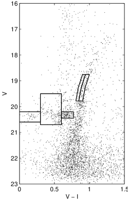
Figure 7: $V,V-I$ colour-magnitude diagram of stars within 20 arcmin of the centre of Sextans (based on archival INT images). Over-plotted are the 5 bins used to define the stellar sub-populations. See text for a detailed discussion.

Figure 8: Top: Surface brightness profile for Sextans together with the best-fitting single-component Plummer law (lower curve) and a Plummer law with a central power-law cusp of index $4.4$ (upper curve). The two curves deviate only inside about 1.6 arcmin where the cusped model rises to fit the innermost data point. Observed data taken from Irwin & Hatzidimitriou (1995). Bottom: Velocity dispersion profile with best-fitting model (central data point omitted from the fit).

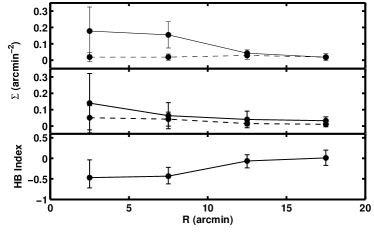
Figure 9: Background-subtracted projected density profiles of the red (solid curve) and blue (broken curve) horizontal branch stars (top) and of the red (solid curve) and blue (broken curve) RGB stars (middle) in Sextans based on INT photometric data. The bottom panel shows the radial variation of the HB morphology index. All three panels show that the composition of the stellar population at the centre of Sextans varies with radius on a scale of about 10 arcmin. See text for a detailed discussion.

3 Modelling

One possible explanation for the observed data would be the presence of a kinematically distinct stellar component at the centre of Sextans. To test this idea further, we use the procedure described in Kleyna et al. (2003) to examine the position-velocity data set for signs of substructure. We scan the face of the dSph with an aperture of radius $5^{\prime}$. At each aperture location, we calculate the likelihood that these velocities are drawn from (i) a single Gaussian with dispersion $\langle v^{2}\rangle=7.97\;{\rm km\,s}^{-1}$ (ii) a velocity distribution in which a fraction $f$ of the stars are drawn from the main Gaussian and the remainder belong to a kinematically distinct population with different mean velocity and dispersion. Only in an aperture centred close to the origin does any model other than the main Gaussian represent a significantly better fit to the velocity data. A model in which all the stars in this aperture belong to a population with velocity dispersion $0.5\;{\rm km\,s}^{-1}$ (and a mean velocity within $2\;{\rm km\,s}^{-1}$ of the bulk motion of the dSph) is about $195$ times more likely than a model in which they belong to the main population. Monte Carlo realisations of our data set demonstrate that the likelihood of observing a spurious cold clump with the same probability ratio at any location in the cluster is relatively high. However, only $4.6$ percent of realisations display a clump with an offset in mean velocity of less than $5\;{\rm km\,s}^{-1}$. We therefore conclude that the central region shows evidence for the presence of a kinematically distinct population at about the $2\sigma$ confidence level.

The light distribution of Sextans displays a sharp central rise (see Irwin & Hatzidimitriou, 1995, and the top panel of Fig. 8). It is tempting to imagine an association between this feature and the cold population. However, the difference in the length scales of the two features means that a direct association is very unlikely. At a radius of 2 arcmin (the radius of our innermost velocity data point) the ratio of the central component to the main component is already less than unity, for any plausible power-law fit to the centre of the light distribution. Thus, if the central density profile were representative of the spatial distribution of the cold population, we would not expect that six of the innermost eight stars in our velocity sample would be cold.

A number of authors have presented evidence for the presence of radial stellar population gradients in Sextans (Harbeck et al., 2001; Lee et al., 2003). In particular, the red horizontal branch (RHB) stars appear to be more centrally concentrated than the blue horizontal branch (BHB) stars. Following these authors, we define five bins in the ($V,V-I$) colour magnitude diagram (CMD) obtained from deep ($V<22.5$) INT imaging of Sextans (see Fig. 7). There are three bins on the horizontal branch (RHB, BHB, RRLyrae) and two bins on the red giant branch (RGB) between V=18.8 and V=19.8. The red RGB bin (RRGB) traces the mean colour of the RGB while the blue bin (BRGB) covers the blue side of the RGB. The number of stars in each bin is corrected for foreground contamination by counting the number of stars in a bin of equal area displaced away from the CMD features associated with Sextans.

In the top panels of Figure 9 we compare the background-subtracted surface density profiles of the red and blue components of the HB and RGB. In agreement with Harbeck et al. (2001) and Lee et al. (2003), we find that the RHB is significantly more centrally concentrated than the BHB. There is also weak evidence that the RRGB is more concentrated than the BRGB. The bottom panel of the Figure shows the radial variation of the HB morphology index $(n_{\rm BHB}-n_{\rm RHB})/(n_{\rm BHB}+n_{\rm RHB}+n_{\rm RRL})$, where $n_{\rm BHB}$, $n_{\rm RHB}$ and $n_{\rm RRL}$ are the numbers of BHB, RHB and RRLyrae stars, respectively (Lee, Demarque, & Zinn, 1990). Within 10 arcmin, the HB is dominated by its red component, while at larger radii, the numbers of red and blue HB stars are comparable. Given the uncertainties in the definitions of the CMD bins in our analysis and the unknown level of contamination of the RHB bins by RRLyraes, the details of these radial variations are not well determined. However, it is clear that the composition of the stellar population at the centre of Sextans varies on a scale of about $5-10$ arcmin.

If both the stellar components of Sextans are tracer populations in a dark matter dominated potential well, then the more concentrated population should have a smaller velocity dispersion. The RGBs of the two populations may be coincident in the CMD and so we would not necessarily expect to see correlations in our velocity data with position on the RGB. However, we note that in the innermost radial bin, the surface density of RHB stars is a factor of 9 higher than that of the BHB stars. It is therefore plausible that within 5 arcmin of the centre we would observe mostly stars associated with the cold component.

One possible origin for the cold, inner population of Sextans is the preferential retention of star-forming gas at the centre of the dSph leading to a younger and/or more metal-rich, centrally concentrated population (Harbeck et al., 2001). An alternative explanation is that the cold central population originated in a star cluster which spiralled to the centre of Sextans under the influence of dynamical friction. During the final stages of this process, the cluster deposited stars in the inner regions of the dSph. It is possible that the central cusp in the light distribution is the final, probably unbound, remnant of this cluster. A similar scenario has been proposed by Oh & Lin (2000) for the origin of nucleated dwarf galaxies.

In addition to providing an explanation for the photometric and kinematic features discussed already, the cluster scenario naturally accounts for the distribution of blue stragglers in Sextans. Lee et al. (2003) noted that the brighter (i.e. more massive) blue stragglers are more centrally concentrated than the fainter ones. As those authors comment, mass-dependent spatial distributions of stars are a generic outcome of mass segregation in stellar systems. However, the time scale for such segregation to occur in Sextans is very long due to the low surface brightness of the stellar population. If a significant fraction of the blue stragglers were formed in a star cluster which subsequently disrupted near the centre of Sextans, mass segregation within the cluster would ensure that the most massive blue stragglers would be the last to be tidally removed from the cluster and hence would have a more concentrated spatial distribution.

If we assume that all the light in the central 10 arcmin is due to cluster debris (as suggested by the dominance of the cold population in the inner regions and the large ratio of RHB to BHB stars inside 10 arcmin) and that the (constant) luminosity density within 10 arcmin is $0.002$L${}_{\odot}\,$pc^-3 (Mateo, 1998), we obtain a luminosity of $1.3\times 10^{5}$L_⊙ for the putative cluster. If the mass to light ratio is about 2 solar units (typical of Galactic globular clusters), then the mass of the cluster is about $3\times 10^{5}$L_⊙. This is comparable to the masses of Galactic globular clusters.

We determine the mass profile of Sextans in the context of the cluster model by assuming a Plummer model for the light distribution, excluding the central point (see Figure 8). Similarly, we remove the central point from the velocity dispersion profile and fit a profile of the form (see Figure 8)

$$\langle v^{2}\rangle(R)=\frac{\langle v^{2}\rangle_{0}}{(1+(R/R_{\rm c})^{\alpha})^{\gamma/\alpha}}$$ (5)

If we further assume isotropy of the velocity dispersion tensor, then the mass within 1 kpc (using the Jeans equation) lies in the range $3\times 10^{7}-1.5\times 10^{8}$M_⊙ – the exact value is sensitive to the form assumed for the outer fall-off in the dispersion. Assuming that the dark matter has an isothermal distribution out to 1 kpc, then the time taken for a cluster of mass $3\times 10^{5}$M_⊙ to spiral to the centre due to dynamical friction would be in the range 0.7-1.5 Gyr (Binney & Tremaine, 1987). Thus, we would expect to find any such cluster at the centre of the Sextans dSph.

We also note that the mass within 10 arcmin ($=250\,$pc) in this model is approximately $2.5\times 10^{6}$M_⊙. Hence, the implied mass to light ratio of the inner regions is roughly 19 solar units. This is much higher than the M/L expected for an old stellar population based on observations of globular clusters (e.g. Parmentier & Gilmore, 2001; Feltzing, Gilmore, & Wyse, 1999). This suggests that the inner regions of Sextans are dark matter dominated, which is consistent with our earlier assumption that the stellar populations in the central regions are not currently self-gravitating.

4 Conclusions

We have presented the radial variation of the velocity dispersion for the Sextans dSph. The behaviour of the velocity dispersion profile at large radii is qualitatively similar to that seen in the Draco and Ursa Minor dSphs (Wilkinson et al., 2004). In those galaxies, the fall-off in the velocity dispersion at large radii coincided with a break in the light distribution and was interpreted as indicative of mild tidal perturbation of the stars. In Sextans, the photometry presented by Irwin & Hatzidimitriou (1995) is of insufficient quality to identify features at $40-50$ arcmin. The interpretation of the fall-off in the outer velocity dispersion of Sextans is unclear, but may be due to the tidal field of the Milky Way.

Intriguingly, the dispersion at the very centre of Sextans is close to zero and this low value is coincident with significant radial gradients in the stellar populations. We suggest that this is caused by the sinking and gradual dissolution of a star cluster at the centre of Sextans. This is consistent with both our inferred mass for Sextans and the estimated timescale for dynamical friction to bring any star cluster to the centre of the Sextans. The model also provides an explanation for the origin of the central cusp in the light distribution and the different spatial distributions of the bright and faint blue stragglers in Sextans. Thus, our hypothesis provides a reasonable explanation of all the observed data, both kinematic and photometric, on the Sextans dSph.

References

- Armandroff & Da Costa (1986) Armandroff T.E., Da Costa G.S. 1986, AJ, 92, 777
- Binney & Tremaine (1987) Binney J., Tremaine S. 1987, Galactic Dynamics, Princeton University Press, Princeton
- Da Costa, Hatzidimitriou, Irwin, & McMahon (1991) Da Costa G. S., Hatzidimitriou D., Irwin M. J., McMahon R. G. 1991, MNRAS, 249, 473
- Feltzing, Gilmore, & Wyse (1999) Feltzing, S., Gilmore, G., & Wyse, R. F. G. 1999, ApJ, 516, L17
- Harbeck et al. (2001) Harbeck, D., et al. 2001, AJ, 122, 3092
- Hargreaves, Gilmore, Irwin, & Carter (1994) Hargreaves J. C., Gilmore G., Irwin M. J., Carter D. 1994, MNRAS, 269, 957 [H94]
- Irwin & Hatzidimitriou (1995) Irwin M., Hatzidmitriou D., 1995, MNRAS, 277, 1354
- Kleyna et al. (2001) Kleyna J.T., Wilkinson M.I., Evans N.W., Gilmore G. 2001, ApJ, 563, L115
- Kleyna et al. (2002) Kleyna J.T., Wilkinson M.I., Evans, N.W., Gilmore G. 2002, MNRAS, 330, 792
- Kleyna et al. (2003) Kleyna J.T., Wilkinson M.I., Gilmore G., Evans N.W. 2003, ApJ, 588, L21
- Lee et al. (2003) Lee, M. G., et al. 2003, AJ, 126, 2840
- Lee, Demarque, & Zinn (1990) Lee, Y., Demarque, P., & Zinn, R. 1990, ApJ, 350, 155
- Mateo (1997) Mateo, M., 1997, in The Nature of Elliptical Galaxies; 2nd Stromlo Symposium, ASP Conf. Ser. 116, 259
- Mateo (1998) Mateo, M. L. 1998, ARA&A, 36, 435
- Oh & Lin (2000) Oh K.S., Lin D.N.C 2000, ApJ, 543, 620
- Parmentier & Gilmore (2001) Parmentier, G. & Gilmore, G. 2001, A&A, 378, 97
- Suntzeff et al. (1993) Suntzeff N.B., Mateo M., Terndrup D.M., Olszewski E.W., Geisler D., Weller W. 1993, ApJ, 418, 208 [S93]
- Tonry & Davis (1979) Tonry J., Davis M. 1979, AJ, 84, 1511
- Wilkinson et al. (2002) Wilkinson M.I., Kleyna, J.T., Evans, N.W., Gilmore G. 2001, MNRAS, 330, 778
- Wilkinson et al. (2004) Wilkinson M.I.,Kleyna J.T., Evans N.W., Gilmore G., 2004, ApJ, 999, L999