An Expanded RXTE Survey of X-ray Variability in Seyfert 1 Galaxies

Abstract

The first seven years of RXTE monitoring of Seyfert 1 active galactic nuclei have been systematically analyzed to yield five homogeneous samples of 2–12 keV light curves, probing hard X-ray variability on successively longer durations from $\sim$1 day to $\sim$3.5 years. 2–10 keV variability on time scales of $\sim$1 day, as probed by ASCA, are included. All sources exhibit stronger X-ray variability towards longer time scales, but the increase is greater for relatively higher luminosity sources. Variability amplitudes are anti-correlated with X-ray luminosity and black hole mass, but amplitudes saturate and become independent of luminosity or black hole mass towards the longest time scales. The data are consistent with the models of power spectral density (PSD) movement described in Markowitz et al. (2003a) and McHardy et al. (2004), whereby Seyfert 1 galaxies’ variability can be described by a single, universal PSD shape whose break frequency scales with black hole mass. The best-fitting scaling relations between variability time scale, black hole mass and X-ray luminosity imply an average accretion rate of $\sim$5$\%$ of the Eddington limit for the sample. Nearly all sources exhibit stronger variability in the relatively soft 2–4 keV band compared to the 7–12 keV band on all time scales. There are indications that relatively less luminous or less massive sources exhibit a greater degree of spectral variability for a given increase in overall flux.

1 Introduction

X-ray observations can provide constraints on the physical conditions in the innermost regions of Seyfert 1 Active Galactic Nuclei (AGNs), as the X-rays are generally thought to originate in close proximity to the putative central supermassive black hole. On the basis of spectroscopic observations, the leading models of the X-ray continuum production are based on a hot, Comptonizing electron or electron-positron pair corona close to the black hole. The exact geometry remains uncertain, though numerous models have been invoked (e.g, Zdziarski et al. 2003), including a neutral accretion disk extending in to the minimum stable orbit and sandwiched by a patchy and possible outflowing corona (e.g., Stern et al. 1995, Svensson 1996, Beloborodov 1999) and a hot inner disk radially surrounded by a cold disk, with a variable transition radius (Shapiro, Lightman & Eardley 1976, Zdziarski, Lubinski & Smith 1999). The corona multiply-upscatters thermal soft photons emitted from the disk to produce an X-ray power-law in the energy range 1–100 keV (e.g., Haardt, Maraschi & Ghisellini 1994). Furthermore, the disk, or some other cold, optically thick material, reprocesses the hard X-rays, as evidenced by the so-called ’Compton reflection humps’ above $\sim$10 keV in Seyfert spectra, as well as strong iron fluorescent lines at $\sim$6.4 keV (Lightman & White 1988, Guilbert & Rees 1988, Pounds et al. 1990).

Seyfert 1 galaxies exhibit rapid, aperiodic X-ray continuum variability for which no fully satisfying explanation has been advanced. Probably the best way to characterize single-band Seyfert variability, if adequate data exist, is to measure the fluctuation power spectral density (PSD) function. Recent studies such as Edelson & Nandra (1999), Uttley, McHardy & Papadakis (2002), Markowitz et al. (2003a), Marshall et al. (2004) and McHardy et al. (2004) measured high-dynamic range broadband PSDs which showed the red-noise nature of Seyfert variability at high frequencies, but flattened below temporal frequencies corresponding to time scales of a few days. Markowitz et al. (2003a) developed a scenario in which all Seyfert 1s have a PSD shape similar to that of X-ray Binaries (XRBs) and which scale towards lower temporal frequency with increasing black hole mass. Physically, this is consistent with a scenario in which relatively more massive black holes host larger X-ray emitting regions, the variability mechanism takes a longer time to propagate through the emission region, and the observed variability is ’slower.’

When data are not adequate to construct a PSD, it is still valuable to quantify the variability amplitude. The well-known anticorrelation between variability amplitude (as quantified over a fixed temporal frequency range) and source luminosity on both short time scales ($\sim$1 d: Barr & Mushotzky 1986; Nandra et al. 1997a, Turner et al. 1999) as well as long time scales ($\sim$300 d: Markowitz & Edelson 2001, hereafter ME01) is consistent with the above physical interpretation.

Numerous X-ray spectral variability studies (e.g., Markowitz, Edelson & Vaughan 2003b; also Nandra et al. 1997a, ME01) have shown the majority of Seyferts to soften as they brighten, with the relatively softer energies displaying stronger variability. It is currently unclear whether this is due to intrinsic slope changes of the coronal power-law continuum (e.g., Lamer et al. 2003a, Uttley et al. 2003) or due to the presence of a much less variable hard component that is likely associated with the Compton reflection hump (e.g. Shih, Iwasawa & Fabian 2002; Taylor, Uttley & McHardy 2003). In contrast to the ’normal’ or ’broad-line’ Seyfert 1’s which show this property, however, some ’Narrow-Line’ or ’soft-spectrum’ Seyfert 1s (characterized by FWHM $<$ 2000 km s^-1, and steep photon indices; e.g., Boller, Brandt & Fink 1996) have been seen to vary with a much weaker dependence on energy compared to broad-line Seyfert 1s (e.g., Edelson et al. 2002, Vaughan et al. 2002).

The archival data accumulated by the Rossi X-ray Timing Explorer (RXTE) during its first seven years of operation permits a study of broadband continuum and spectral variability behavior on time scales ranging from days to years. The long-term variability survey of ME01 was the first to systematically probe X-ray variability on such long time scales, examining nine Seyfert 1 light curves each of 300 days in duration. This paper expands that survey to cover additional time scales and sources using additional archival RXTE data. In this paper we test the relation between X-ray variability and black hole mass, including the idea of broadband PSD movement with black hole mass, and exploring spectral variability throughout Seyfert 1s. The source selection and data reduction are described in $\S$2. The sampling and analysis are described in $\S$3. The results are discussed in $\S$4, and a short summary is given in $\S$5. An Appendix briefly explores if the modeled RXTE PCA background has any significant effect on the measured variability properties for low count rate or steep-spectrum sources.

2 Data Collection and Reduction

RXTE has observed $\sim$55 Seyfert 1 galaxies during the first seven years of its mission. Data taken through most of Cycle 7 had turned public by 2004 February, when these analyses were performed. This paper considered these data as well as the authors’ proprietary observations of three Seyfert 1 galaxies observed during Cycle 8. $\S$2.1 details how the RXTE data were reduced.

The observational approach of this project was to obtain monitoring on multiple long time scales, sampled as uniformly as possible for as many Seyfert 1 galaxies as possible. Using the available archive of RXTE data to optimize this trade-off yielded a sample of 27 Seyfert 1s suitable for analysis on at least one of the time scales of interest, 1 d, 6 d, 36 d, 216 d, or 1296 d. Additionally, most of these sources also had adequate short time scale (1 d) ASCA data publicly available. Most of the sources with data on the 36 d, 216 d, and 1296 d time scales have had their PSDs measured or are currently undergoing monitoring for future PSD measurement. $\S$2.2 and $\S$2.3 detail construction of the RXTE and ASCA light curves, respectively.

2.1 RXTE data reduction

All of the RXTE data were taken with the Proportional Counter Array (PCA), which consists of five identical collimated proportional counter units (PCUs; Swank 1998). For simplicity, data were collected only from those PCUs which did not suffer from repeated breakdown during on-source time (PCUs 0, 1, and 2 prior to 1998 December 23; PCUs 0 and 2 from 1998 December 23 until 2000 May 12; PCU 2 only after 2000 May 12). Count rates quoted in this paper are normalized to 1 PCU. Only PCA STANDARD-2 data were considered. The data were reduced using standard extraction methods and FTOOLS v5.2 software. Data were rejected if they were gathered less than 10$\arcdeg$ from the Earth’s limb, if they were obtained within 30 min after the satellite’s passage through the South Atlantic Anomaly (SAA), if ELECTRON0 $>$ 0.1 (ELECTRON2 after 2000 May 12), or if the satellite’s pointing offset was greater than 0$\fdg$02.

As the PCA has no simultaneous background monitoring capability, background data were estimated by using pcabackest v2.1e to generate model files based on the particle-induced background, SAA activity, and the diffuse X-ray background. This background subtraction is the dominant source of systematic error in RXTE AGN monitoring data (e.g., Edelson & Nandra 1999). Unmodelled variations in the instrument background are usually less than 2 percent of the total observed (sky plus instrument) background at energies less than 10 keV (Jahoda et al., in prep.). Ignoring the statistical uncertainty (there was adequate signal-to-noise in all observations), a systematic uncertainty of $\lesssim$2 per cent should thus be kept in mind for all fluxes. Counts were extracted only from the topmost PCU layer to maximize the signal-to-noise ratio. All of the targets were faint ($<$ 40 ct s^-1 PCU^-1), so the applicable ’L7-240’ background models were used. Because the PCU gain settings changed three times since launch, the count rates were rescaled to a common gain epoch (gain epoch 3) by calibrating with several public archive Cas A and Crab observations. Light curves binned to 16 s were generated for all targets over the 2–12 keV bandpass, where the PCA is most sensitive and the systematic errors and background are best quantified. Light curves were also generated for the 2–4 and 7–12 keV sub-bands. The data were binned on the orbital time scale; orbits with less than ten 16-second bins were rejected. Errors on each point were obtained from the standard deviations of the data in each orbital bin. Further details of RXTE data reduction can be found in e.g., Edelson & Nandra (1999).

2.2 RXTE sampling

The observational approach of this project was to quantify the continuum variability properties of Seyfert 1 galaxies on multiple time scales. This required assembling samples that were, to the greatest degree possible, uniformly monitored for proper comparison between sources. Sources with a weighted mean count rate significantly below 1 ct s^-1 PCU^-1 over the full 2–12 keV bandpass were rejected to minimize the risk of contamination from faint sources in the field-of-view, to ensure adequate signal-to-noise, and to minimize the influence of systematic variations in the modeled X-ray background.

The sampling of the publicly available data was highly uneven in general. The original observations were made with a wide variety of science goals, leading to a variety of sampling patterns and durations. This required us to clip light curves to common durations and resample at similar rates in order to produce samples with homogeneous sampling characteristics. For each total light curve, optimum windows of 1 d, 6 d, 36 d, 216 d, and 1296 d (evenly-spaced in the logarithm by a factor of 6) were selected. Given the original sampling patterns, these windows represented a reasonable spread in temporal frequency coverage, and yielded a reasonably-sized sample on each time scale. For each time scale, light curves shorter than the optimum window were rejected. Light curves with long gaps ($>$$1/3$ of the total duration) within the window were also rejected. Such gaps reduce the statistical significance of parameters derived over the full duration, and interpolating across such large gaps would result in an underestimate of the true variability amplitude. For each source, as many usable light curves as possible on each of the five time scales were selected from the total light curves. In NGC 3227, there was a significant hardening of the spectrum during approximately MJD 51900–52000, consistent with a temporary increase in cold absorption due to a dense cloud passing along the line of sight (Lamer, Uttley & McHardy 2003b); these data were excluded.

To extract light curves that were sampled as uniformly as possible, the light curves were resampled on each of the five time scales with a common, optimized rate. This was done using an algorithm which selected only data points in the original light curve that were separated as close as possible to the resampling rate ${\Delta}T_{{\rm samp}}$, where ${\Delta}T_{{\rm samp}}$ was 5760 sec (1 satellite orbit), 0.27 d (4 satellite orbits), 1.6 d, 5.3 d and 34.4 d for the 1, 6, 36, 216, and 1296 d light curves, respectively. Starting with the first data point observed (at time $t_{1}$), the algorithm selected the data point observed closest to times $t_{2}$= $t_{1}$ + ${\Delta}T_{{\rm samp}}$, … , $t_{N}$ = $t_{N-1}$ + ${\Delta}T_{{\rm samp}}$, where N is the number of points in the final, resampled light curve. For light curves that were observed with overlapping sampling patterns, portions of intense monitoring were not treated differently from the rest of the light curve. That is, the algorithm did not do any averaging (in bins of size ${\Delta}T_{{\rm samp}}$) during times of intensive monitoring, as that would yield reduced variability during that period only relative to the rest of the light curve. This allowed the entire light curve to sample the variability in a uniform fashion. Resampling at rates longer than ${\Delta}T_{{\rm samp}}$ would have resulted in too few points in each final light curve, while resampling at significantly more frequent rates would have resulted in light curves that were not sufficiently uniform, given the original range of observing patterns. The final light curves were also required to contain at least $\sim$20 points ($\sim$15 on the 1 d time scale) in order to obtain an accurate estimate of the variability amplitude as quantified below; those light curves with fewer points were discarded. Light curves with poor signal to noise (i.e., due to mean count rates significantly less than 1.0) were discarded. Given that many sources were observed with overlapping sampling patterns, the final light curves for a given source often share data points on multiple time scales and are not completely independent.

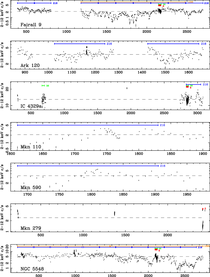
Figure 1: Figure 1, cont’d.

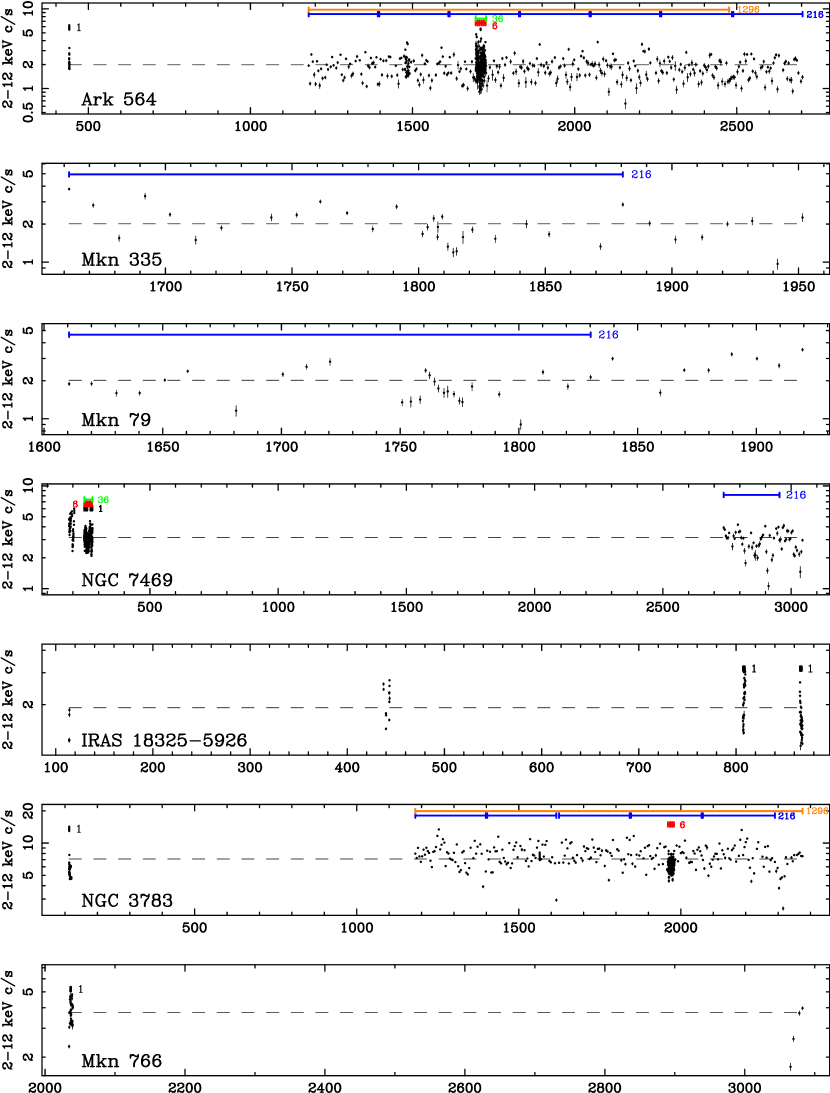
Figure 1: Figure 1, cont’d.

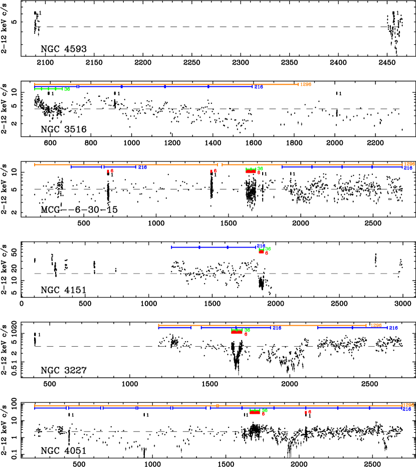
Figure 1: Figure 1, cont’d.

This reduction yielded a total of 27 sources with sampling on each at least one of the five RXTE time scales. This included 86 observations of 18 sources on the 1 d time scale, 68 observations of 12 sources on the 6 d time scale, 19 observations of 12 sources on the 36 d time scale, 78 observations of 19 sources on the 216 d time scale, and 12 observations of 9 sources on the 1296 d time scale. Figure 1 shows the full 2–12 keV RXTE light curves for all 27 sources, before resampling, and showing the boundaries of the sampling windows. Table 1 lists source observation parameters, including 2–12 keV luminosity $L_{2-12}$ and black hole mass estimate $M_{{\rm BH}}$, and sampling parameters. All source luminosities were calculated using the global mean RXTE count rate and using the HEASARC’s online WebPIMMS v.3.4 flux converter assuming an intrinsic power-law with a photon index obtained from either previously published spectral fits (e.g., Kaspi et al. 2001, Pounds et al. 2003) or the online TARTARUS database of ASCA AGN observations (e.g., Nandra et al. 1997a; Turner et al. 1999). Luminosities were calculated assuming $H_{o}$ = 70 km s^-1 Mpc^-1 and $q_{o}$ = 0.5. All black hole mass estimates are reverberation-mapped masses from Kaspi et al. (2000) and Wandel, Peterson & Malkan (1999) except NGC 4051, from Shemmer et al. (2003), NGC 3783, from Onken & Peterson (2002), NGC 4593, NGC 3516 & NGC 3227, from Onken et al. (2003), and Mkn 279, from Wandel (2002) and Santos Lleo et al. (2001). Mass estimates for Ark 564, Mkn 766, MCG–6-30-15, MCG–2-58-22 are from Bian & Zhao (2003) and the mass estimate for PKS 0558–504 is from Wang et al. (2001); these latter two works use the empirical Kaspi et al. (2000) relation between optical luminosity and BLR size. No reliable mass estimate exists for 3C 111 or IRAS 18325–5926.

2.3 ASCA data

Short-term ASCA 2–10 keV light curves were obtained from the TARTARUS database for the sources with RXTE data. The count rates in the light curves provided had been combined and averaged between ASCA’s two Solid-state Imaging Spectrometers (SIS; Burke et al. 1994, Gendreau 1995) and binned to 16 s. For each source, all available light curves longer than 1 d in duration were selected from the database; otherwise the longest light curve $>$60 ksec in duration was used. The light curves were binned on orbital time scales, yielding 51 light curves of 11–15 consecutive orbital bins for 21 sources. Background light curves were similarly binned and subtracted to produce net count rate light curves. Table 2 lists source observation and sampling parameters for the ASCA data.

3 Analysis

3.1 Quantifying variability amplitudes

Fractional variability amplitudes ($F_{var}$; e.g., Vaughan et al. 2003b, Edelson et al. 2002) were measured for each light curve to quantify the intrinsic variability amplitude relative to the mean count rate and in excess of the measurement noise;

$$F_{var}=\sqrt{S^{2}-\langle\sigma_{err}^{2}\rangle\over\langle X\rangle^{2}},$$ (1)

where $S^{2}$ is the total variance of the light curve, $\langle\sigma_{err}^{2}\rangle$ is the mean error squared and $\langle X\rangle$ is the mean count rate of $N$ total points. The error on $F_{var}$ is

$$\sigma_{F_{var}}=\sqrt{\left\{\sqrt{\frac{\langle\sigma_{err}^{2}\rangle}{N}}\cdot\frac{1}{\langle X\rangle}\right\}^{2}+\left\{\sqrt{\frac{1}{2N}}\cdot\frac{\langle\sigma_{err}^{2}\rangle}{\langle X\rangle^{2}F_{var}}\right\}^{2}}$$ (2)

as discussed in Vaughan et al. (2003b); this error formulation estimates $\sigma_{F_{var}}$ based on random errors in the data itself, and not due to random variations associated with red-noise processes.

In any red-noise stochastic process there will be random scatter in independent estimates of the variance or $F_{var}$ over multiple realizations of the process. This is a form of ”weakly non-stationary” behavior inherent in red-noise variability processes. Herein, we adopt the definition of weak non-stationarity as a description of a variability process whose mean and variance show scatter over multiple realizations, but whose underlying PSD remains constant over time, with expectation values of $F_{var}$, $\langle$$F_{var}$$\rangle$, remaining constant over time as well (e.g., Vaughan et al. 2003b). In other words, while the expectation value of the square of $F_{var}$ is equal to the integrated PSD of the underlying variability process, multiple independent realizations of that process will yield a range in estimates of $F_{var}$ even if the PSD does not change amplitude or shape and $\langle$$F_{var}$$\rangle$ is constant. Factors of 3 or more in the range of $F_{var}$ are not uncommon (e.g., Vaughan et al. 2003b). Scatter in $F_{var}$ is therefore not necessarily indicative of strongly non-stationary behavior. For multiple RXTE or ASCA light curves for a given source and time scale, the values of $F_{var}$ were averaged, with the uncertainty on the average $F_{var}$ determined statistically. However, one needs at least 10–20 independent estimates of $F_{var}$ to adequately test if those estimates are consistent with their expectation value $\langle$$F_{var}$$\rangle$ (see Vaughan et al. 2003b for detailed descriptions of such tests). There are only three objects with enough data for this relatively strong test, NGC 7469, IRAS 18325–5926 and MCG–6-30-15 on the 1 d time scales (with the RXTE 2–12 keV and ASCA 2–10 keV values considered together); in all three cases at least 70$\%$ of the individual values of $F_{var}$ are consistent with $\langle$$F_{var}$$\rangle$. For the rest of the sample, when multiple estimates of $F_{var}$ were made, the measured values were usually reasonably close to $\langle$$F_{var}$$\rangle$. This is consistent with weakly non-stationary behavior. Thus, these values of $F_{var}$ are used hereafter.

A linear relation between absolute rms variability amplitude and flux has been observed in XRBs (Uttley & McHardy 2001) and Seyfert 1s (Edelson et al. 2002, Vaughan, Fabian & Nandra 2003a). This is a form of non-stationary behavior (independent of the weak non-stationarity discussed above), as the expectation value of the variance is not constant over time. Quantifying variability using $F_{var}$ removes this trend; since the rms–flux relation slope is generally seen to be close to 1, $F_{var}$ thus would be independent of flux level in the absence of additional sources of non-stationarity.

Table 3 lists $F_{var}$ for each RXTE light curve over the 2–12 keV, 2–4 keV and 7–12 keV bands. Table 4 lists $F_{var}$ measured over the 2–10 keV band for the ASCA data.

3.2 Construction of correlation diagrams

Figures 2a and 2b displays the values of the logarithm of $F_{var}$ plotted against $L_{2-12}$ and $M_{{\rm BH}}$. $F_{var}$ itself will not follow a Gaussian distribution, but the logarithm of $F_{var}$ does follow a distribution that crudely resembles a Gaussian for red-noise PSD slopes of $=sim$–1 to –2 (see, e.g., Fig. 8 of Vaughan et al. 2003b). The ASCA data are included and agree well with the 1-d RXTE data; one should not expect any significant difference between parameters derived over the 2–10 and 2–12 keV bands. Best-fitting power-law slopes for each data set were determined using the Akritas & Bershady (1996) regression, which accounts for measurement errors and intrinsic scatter; the slopes are listed in Table 5. The Spearman rank correlation coefficients $r$ and probability $P_{r}$ of obtaining those values of $r$ by chance are also listed in Table 5. Also listed in Table 5 is reduced chi-squared $\chi^{2}_{r}$, calculated using the best-fit power-law. Because the uncertainties on $F_{var}$ were calculated in linear space, when calculating $\chi^{2}_{r}$, the uncertainties in log space were replaced by the average error for all five time scales, 0.047 in the log and 0.044 in the log for the $F_{var}$–$L_{2-12}$ and $F_{var}$–$M_{{\rm BH}}$ relations, respectively, to avoid unnecessarily weighting $\chi^{2}$ towards the longer time scales.

For both sets of relations, the values of $r$ are all negative, with the absolute values of $r$ decreasing slightly towards longer time scales. Such anticorrelations have been observed previously in AGNs for $\sim$1 d time scales (Green, McHardy & Lehto 1993, Nandra et al. 1997a; O’Neill et al. 2004). However, the slopes and normalizations of the best-fitting logarithmic power law for each data set differ: the slopes generally flatten towards longer time scales. The 1-d and 216-d time scale $F_{var}$–$L_{2-12}$ relations are generally consistent with the 1 d and 300 d relations of ME01. For both sets of relations, for all objects, the values of $F_{var}$ generally increase towards longer time scales, leveling off somewhat beyond approximately the 36 d time scale relation, but the highest mass and highest luminosity sources show the largest increase. Formally, the fits to all of the best-fit lines are quite poor, but using the $\chi^{2}_{r}$ values as a measure of intrinsic scatter, the 1 d RXTE $F_{var}$–$M_{{\rm BH}}$ relation shows lower scatter than the corresponding $F_{var}$–$L_{2-12}$ relation, but the scatter is greater in the $F_{var}$–$M_{{\rm BH}}$ relation in each of the remaining five data sets. The sum of all six $\chi^{2}_{r}$ values is also greater for the $F_{var}$–$M_{{\rm BH}}$ relations. Within each plot, reduced chi-squared tends to decrease towards longer time scales, implying greater intrinsic scatter on the shortest time scales.

It can be seen from the values of $F_{var}$ listed in Table 3 that most observations (56/68) show stronger variability in the 2–4 keV band compared to the 7–12 keV band. Formally, the null hypothesis of the 2–4 keV and 7–12 keV excess variances (square of the $F_{var}$) being consistent is rejected using an F-test at $>$90$\%$ significance in 12 observations and $>$95$\%$ significance in 8 observations. The correlation diagram for 2–4 keV $F_{var}$ ($F_{var,soft}$) versus 7–12 keV $F_{var}$ ($F_{var,hard}$) for all five RXTE data sets is shown in Figure 3. $F_{var,soft}$ and $F_{var,hard}$ are well-correlated on all time scales. However, it can be seen that the vast majority of points lie to the right of the dashed line which represents equal variability in the two bands. This shows again that most sources exhibit stronger variability in the relatively softer band. Values of the Spearman rank correlation coefficient and probabilities are listed in Table 5. Best-fitting power-law slopes were determined using the Akritas & Bershady (1996) regression. There is no obvious indication that the degree of spectral variability exhibited is dependent on the time scale probed. There is no obvious scatter trend with time scale, judging from the $\chi^{2}_{r}$ values.

Figure 4 shows the ratio of $\frac{F_{var,soft}}{F_{var,hard}}$, 2–4 keV $F_{var}$ / 7–12 keV $F_{var}$, plotted against $L_{2-12}$ for all five RXTE data sets. The best-fitting slopes, obtained using the Akritas & Bershady (1996) method, and values of Spearman rank $r$ and $P_{r}$ are listed in Table 5. Also listed in Table 5 are the slopes and correlation coefficients for $\frac{F_{var,soft}}{F_{var,hard}}$ versus $M_{{\rm BH}}$ (not plotted). The best-fitting slopes are all roughly similar; the slopes might be taken as tentative evidence for relatively less luminous or less massive sources to be more strongly variable in the soft band. There is no obvious indication that the degree of spectral variability exhibited is dependent on the time scale probed. Judging from the $\chi^{2}_{r}$ values, there is no obvious scatter trend with time scale with either $L_{2-12}$ or $M_{{\rm BH}}$. The respective sums of the five $\chi^{2}_{r}$ values are approximately equal, implying roughly equal scatter in the $\frac{F_{var,soft}}{F_{var,hard}}$–$L_{2-12}$ and $\frac{F_{var,soft}}{F_{var,hard}}$–$M_{{\rm BH}}$ relations.

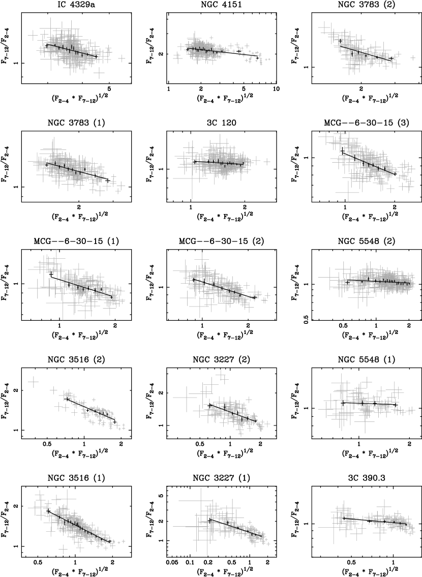
Figure 5: Plots of the 7–12 keV/2–4 keV hardness ratio (HR) against geometric mean count rate for the 27 light curves with adequate data. Gray error bars represent the unbinned data; black points represent the binned data. The solid lines are the best linear fits to the binned data.

Color-flux diagrams, in the which the logarithm of the 7–12 keV / 2–4 keV count rate hardness ratio (HR) is plotted against the logarithm of the geometric mean of the count rates in these two bands, are shown in Figure 5. To minimize the effects of changes in spectral response due to PCA gain epoch changes, only the largest number of points within a single gain epoch was selected for each source. Light curves of $\sim$300 days in duration, with no resampling, were used; light curves with less than 70 points were discarded. This yielded a sample of 27 light curves for 14 sources; date ranges are listed in Table 6. For each source, the data were sorted by increasing geometric mean and grouped into bins of 16 points; the highest flux bin was ignored if it contained less than 10 points. For most sources, the data form a continuous, well-defined region. It is clear from these diagrams as well that nearly all sources soften as they brighten. The two exceptions, which show either a slight hardening or no spectral variability with flux, are the NLSy1 Ark 564 and the radio-quiet quasar PG 0804+761, as has been reported previously (Edelson et al. 2002; Papadakis, Reig & Nandra 2003). Also shown in Figure 5 is the best fitting linear fit to the binned data. Table 6 lists the mean hardness ratio values $\langle$HR$\rangle$ for each source. For the sample as a whole, the average of the 27 mean hardness ratios is 1.06. Ten sources’ $\langle$HR$\rangle$ values are within 20$\%$ of the sample average. However, two sources are notably softer, the soft-spectrum source Ark 564 and the quasar PG 0804+761, both of which are usually measured to have relatively steep photon indices (e.g., Leighly 1999; Papadakis, Reig & Nandra 2003). Three sources, NGC 3227, NGC 3516, and NGC 4151, are notably harder; these sources are frequently measured to have relatively flat photon indices (e.g., Nandra et al. 1997b; George et al. 1998).

Also listed in Table 6 is a parameter derived directly from the slope $m$ of the best linear fit, $\phi$ = 2.0^-m, which quantifies the decrease in HR for every doubling in geometric mean count rate. Multiply-measured values of $\langle$HR$\rangle$ and $\phi$ for a given object tend to be consistent with each other, suggesting that sources do not undergo any radical changes in spectral variability behavior over times scales of one or two years. $\phi$ is greater than 1 for all sources except PG 0804+761 and Ark 564. It is noted that these two sources have the lowest 7–12 keV mean count rates in the sample ($\sim$0.3 c/s/PCU). As discussed in more detail in the Appendix, it is conceivable that systematic variations in the modeled background may contribute greatly to the observed variability at such low flux levels, particularly in the 7–12 keV band. The RXTE data for PG 0804+761 and Ark 564 will therefore not be considered further here.

Figure 6 shows $\phi$ plotted against $L_{2-12}$ and $M_{{\rm BH}}$. The Spearman rank correlation coefficients are given in Table 5. The best-fit lines in Figure 6 were again calculated using the method of Akritas & Bershady (1996). The best-fitting slopes, listed in Table 5, are negative, indicating that relatively less luminous or less massive sources display a stronger degree of spectral variability per given increase in overall flux. To estimate the scatter, $\chi^{2}$ was evaluated for each plot and is listed in Table 5; formally, the fits to the lines are quite poor, but reduced $\chi^{2}$ is slightly lower in the $\phi$–$M_{{\rm BH}}$ plot.

It is noted that other studies (Edelson et al. 2002; Papadakis, Reig & Nandra 2003) have found Ark 564 and PG 0804+761 to show hardness ratios that are independent of flux, which would imply values of $\phi$ close to 1. It is noted that in both sources, this value would lie reasonably close to the observed $\phi$–$L_{2-12}$ anticorrelation. Additionally, the high-mass PG 0804+761 would lie close to the $\phi$–$M_{{\rm BH}}$ anticorrelation; however, Ark 564 would be a significant outlier if added to the $\phi$–$M_{{\rm BH}}$ anticorrelation.

4 Discussion

When one uses the fractional variability, $F_{var}$, as a description of the intrinsic, underlying variability process, certain caveats must be kept in mind when red-noise processes are relevant. Each light curve is an independent realization of the underlying stochastic process and there will be random fluctuations in the measured variance. However, in the absence of evidence for strongly non-stationary behavior in Seyfert light curves (e.g., $\S$3.1, Markowitz et al. 2003a, Vaughan et al. 2003b), it is assumed hereafter that the values of $F_{var}$ are reasonable quantifications of the intrinsic variability amplitude. The reader must keep in mind the previously discussed limitations when considering such small numbers of $F_{var}$ estimates.

The anticorrelations between variability amplitude and source luminosity and between variability amplitude and black hole mass seen in previous surveys are confirmed here on short time scales. In both sets of anticorrelations, the best-fitting power-law slopes gradually decrease towards longer time scales. The $F_{var}$ values tend to increase towards longer time scales, however, they tend to saturate beyond the 36 d time scale. Consequently, the increase in $F_{var}$ is greatest for the higher luminosity sources. As will be discussed in $\S$4.1, this trend is consistent with a scaling of PSD break frequency with some fundamental parameter, most likely $M_{{\rm BH}}$. All of the sources exhibit stronger variability towards relatively softer energies. Additionally, sub-band $F_{var}$ values and color–flux diagrams indicate that less luminous sources have a tendency to exhibit more spectral variability overall. These spectral variability characteristics are discussed in the context of simple X-ray reprocessing models in $\S$4.2.

4.1 The variability–luminosity–$M_{{\rm BH}}$ relationship

Recent PSD studies have yielded PSD breaks on time scales of a few days or less; generally, the power-law slopes flatten from $\sim$–2 above the break to $\sim$–1 below the break. Markowitz et al. (2003a) developed a picture in which all Seyfert 1 PSDs have the same shape but whose high-frequency break time scales $T_{{\rm b}}$ scale linearly in temporal frequency with $M_{{\rm BH}}$. This is consistent with observed anticorrelations between $F_{var}$ and $M_{{\rm BH}}$ (Papadakis 2004, O’Neill et al. 2004) and $F_{var}$ and X-ray luminosity (e.g., Nikolajuk et al. 2004). Interestingly, though, the PSD break frequencies appeared to be less correlated with 2–10 keV X-ray luminosity. There are not adequate data to construct high dynamic range PSDs for all targets in the current sample. However, it is reasonable to assume that all Seyferts have similar PSD shapes with breaks. Given the ranges of luminosity and black hole masses spanned by the sample, it is reasonable to assume that the longest time scales probes in this survey are exploring variability on temporal frequencies well below the breaks in most or all of the sources. This would then explain why the variability amplitudes observed tend to saturate at similar levels on the longest time scales probed, strongly reducing the dependence of $F_{var}$ on $M_{{\rm BH}}$ or $L_{2-12}$. However, the data are not able to highly constrain if objects’ PSDs contain a second, low-frequency break, due to the saturation of $F_{var}$.

Using the values of $F_{var}$ measured here, it is possible to further test this picture. By scaling the break frequency of a broken power-law model PSD with $M_{{\rm BH}}$, the resulting predicted values of $F_{var}$ can be compared to the observed $F_{var}$ values on each of the five time scales to quantitatively constrain the $T_{{\rm b}}$–$M_{{\rm BH}}$ relation. Additionally, scaling the break frequency of a model PSD with luminosity can similarly constrain the relation between $T_{{\rm b}}$ and $L_{2-12}$ (the bolometric and X-ray luminosities can be related as approximately $L_{{\rm bol}}$=27$L_{2-12}$; Padovani & Rafanelli 1988).

For both of these tests, it was assumed that all Seyferts have the same singly-broken PSD shape $P(f)$ described by $P(f)=A(f/f_{b})^{-1}$ (for $f<f_{b}$), or $P(f)=A(f/f_{b})^{-2}$ (for $f>f_{b}$). $A$ is the PSD normalization at the high-frequency break $f_{b}$, calculated as 0.01 (Hz^-1)/$f_{b}$, a relation estimated from the $A$–$M_{{\rm BH}}$ and $T_{{\rm b}}$–$M_{{\rm BH}}$ plots of Markowitz et al. (2003a; their figures 12 and 13). A linear scaling between $T_{{\rm b}}$ and $M_{{\rm BH}}$ (or $L_{2-12}$) was assumed. The $F_{var}$ values were calculated by integrating the PSD between the temporal frequencies of 1/$D$ (where $D$ is 1, 6, 36, 216, or 1296 days) and 1/2${\Delta}T_{{\rm samp}}$. The values of $F_{var}$ measured from the observed light curves contain additional contributions to the total variability due to aliasing, which arises from the non-continuous sampling, and red-noise leak, which arises due to the presence of variability on time scales longer than those sampled. The reader is referred to Uttley, McHardy & Papadakis (2002) or Markowitz et al. (2003a) for detailed descriptions of these distortion effects inherent in PSD measurement and variability analysis. The contribution to the total variance from aliasing was estimated analytically by integrating the model PSD from a frequency of 1/(2${\Delta}T_{{\rm samp}}$) to a frequency of 1/(2000 s); no contribution to the aliased power is expected from variations on time scales shorter than $\sim$2000 s. Monte Carlo simulations were carried out to estimate the contribution to the total variance from red-noise leak. For each model PSD, a light curve of length 50$D$, where $D$ is the observed light curve duration, was simulated and split into 50 light curves each of length $D$ to ensure that variability power from red-noise leak was present on the same time scales probed by the observations (time scales shorter than $D$). The average variance of these 50 light curves was calculated and compared to the estimated intrinsic (i.e., no red-noise leak present) variability estimated above to estimate the variability contribution from red-noise leak.

In order to more directly study the link between the $T_{{\rm b}}$–$M_{{\rm BH}}$ and $T_{{\rm b}}$–$L_{2-12}$ relations and $F_{var}$, it was necessary to remove the influence of the PSD amplitude $A$ at the break on $F_{var}$. The accumulation of Seyfert PSDs supports a range in the observed values of $A$ (e.g., Uttley et al., in prep.). To remove the dependence of the $T_{{\rm b}}$–$M_{{\rm BH}}$ and $T_{{\rm b}}$–$L_{2-12}$ relations on $A$, the ratios $R_{Fvar}$ of values of 2–12 keV $F_{var}$ on six combinations of time scales ($R_{1/6}$, denoting $F_{var}$(1 d) / $F_{var}$(6 d), $R_{1/36}$, $R_{1/216}$, $R_{1/1296}$, $R_{6/216}$, $R_{6/1296}$) were considered. The remaining four model ratios are all relatively flat across the ranges of $M_{{\rm BH}}$ and $L_{2-12}$ considered. They do not provide constraints on scaling and fitting the model $F_{var}$ ratio lines, and are therefore excluded from analysis.

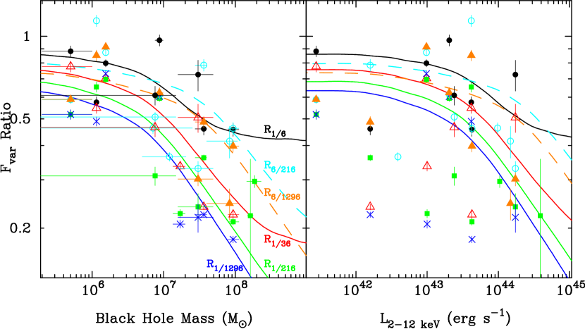
Figure 7: Predicted and measured ratios of $F_{var}$ for six time scale combinations plotted against black hole mass estimate $M_{{\rm BH}}$ (left) and 2–12 keV luminosity (right). The solid lines and dotted lines denote the model $F_{var}$ ratios, derived from linearly scaling the PSD break frequency with black hole mass using the best-fit relation T_b=$M_{{\rm BH}}$/10^6.7$\rm\thinspace M_{\odot}$. The model ratios for the $F_{var}$ ratio –$L_{2-12}$ plot were derived from linearly scaling PSD break frequency with X-ray luminosity using the best-fit relation T_b=$L_{2-12~{}keV}$/10^43.5 erg s^-1. The black, red, green, and blue solid lines mark the model $F_{var}$ ratios $R_{1/6}$, $R_{1/36}$, $R_{1/216}$ and $R_{1/1296}$, respectively, where e.g., $R_{1/6}$ denotes the ratio $F_{var}$(1 d) / $F_{var}$(6 d). The ratios $R_{6/216}$, $R_{6/1296}$ are marked by cyan and orange dotted lines, respectively. Note that, as one scales a PSD towards higher temporal frequencies, $F_{var}$ measured over a fixed time scale (fixed sampling window in the frequency domain) will increase, but at a faster rate for relatively shorter sampling time scales. The model ratios hence follow $R_{1/6}$ $>$ $R_{1/36}$ $>$ $R_{1/216}$ $>$ $R_{1/1296}$ (the black, red, green, and blue curves, respectively), $R_{6/36}$ $>$ $R_{6/216}$ $>$ $R_{6/1296}$ (not plotted, cyan, and orange, respectively), etc. Note also that the $F_{var}$ ratio will tend to flatten off at high frequencies when both sampling time scales are much shorter than the PSD break time scale; i.e., this is why $R_{1/6}$ flattens off at high mass/ low frequencies. The measured ratios of $R_{1/6}$, $R_{1/36}$, $R_{1/216}$, $R_{1/1296}$, $R_{6/216}$, $R_{6/1296}$, are denoted by black filled circles, red open triangles, green filled squares, blue crosses, cyan open circles and orange filled triangles, respectively.

The ratios of predicted $F_{var}$ values are plotted as solid lines as a function of $M_{{\rm BH}}$ and $L_{2-12}$ in Figures 7a and 7b, respectively. No arbitrary scaling in the y-direction of the resulting values of $R_{Fvar}$ was done. Also plotted are the ratios of observed $F_{var}$ values; observed values of $F_{var}$ on the 1 d time scale were combined between the ASCA and RXTE data sets by averaging multiple values for each source. The predicted $R_{Fvar}$ functions were simultaneously best-fit in the x-direction. The fits indicate that the best-fit linear PSD scaling for Figure 7a requires the relation $T_{{\rm b}}$ (days) = $M_{{\rm BH}}$/10^6.7$\rm\thinspace M_{\odot}$. The fit is formally quite poor, with $\chi^{2}_{r}$ equal to 57.1 for 48 degrees of freedom. For Figure 7b, the linear PSD scaling required is $T_{{\rm b}}$ (days) = $L_{2-12}$/ (10^43.5 erg s^-1), with $\chi^{2}_{r}$ equal to 490.2 for 48 degrees of freedom. The modeling is better overall for the $T_{{\rm b}}$–$M_{{\rm BH}}$ relation compared to the $T_{{\rm b}}$–$L_{2-12}$ relation, given the respective values of $\chi^{2}_{r}$. These two best-fitting relations together suggest that the average accretion rate for the entire sample is $\sim$5$\%$ of the Eddington limit.

McHardy et al. (2004) suggested that the normalization of a linear $T_{{\rm b}}$–$M_{{\rm BH}}$ relation may be dependent on some other parameter, possibly the accretion rate. Under the assumption that the reverberation masses are accurate, the picture emerging from PSD measurement seems to be revealing a bifurcation in Seyfert PSDs. It appears that the PSD breaks of some Seyferts lie close to a $T_{{\rm b}}$–$M_{{\rm BH}}$ scaling that is approximately quantified as $T_{{\rm b}}$ (days) = $M_{{\rm BH}}$/10^6.5$\rm\thinspace M_{\odot}$ (e.g., NGC 3516, NGC 4151, and NGC 3783; Markowitz et al. 2003a). This relation extrapolates 6–7 orders of magnitude to the PSD break of Cyg X-1 in the low/hard state. Other sources (NGC 4051 and possibly other Narrow-Line Seyfert 1s, McHardy et al. 2004) seem to require a $T_{{\rm b}}$–$M_{{\rm BH}}$ scaling that is approximately $T_{{\rm b}}$ (days) = $M_{{\rm BH}}$/10^7.5$\rm\thinspace M_{\odot}$. This relation extrapolates to the PSD break of Cyg X-1 in the high/soft state, arguing some connections between these Seyfert s XRBs in the high/soft state. The best-fitting linear $T_{{\rm b}}$–$M_{{\rm BH}}$ relation derived from the present sample lies in between these two scalings, though much closer to the low/hard state scaling, $T_{{\rm b}}$ (days) = $M_{{\rm BH}}$/10^6.5$\rm\thinspace M_{\odot}$ relation. This is consistent with the idea that the present sample contains a mixture of sources from the two groups, but the number of sources that scale with Cygnus X-1’s high/soft state is a small fraction of the whole sample. Ignoring the five known high/soft state PSD sources (NGC 4051; MCG–6-30-15; NGC 3227, Uttley et al., in prep.; Ark 120, Marshall et al. 2003; PG 0804+761, Papadakis, Reig & Nandra 2003) indeed gives a slightly lower scaling constant in the best-fitting $T_{{\rm b}}$–$M_{{\rm BH}}$ relation, $T_{{\rm b}}$ (days) = $M_{{\rm BH}}$/10^6.6$\rm\thinspace M_{\odot}$ ($\chi^{2}_{r}$ = 59.4 for 28 degrees of freedom).

As mentioned previously, the large amount of scatter inherent in $F_{var}$ complicates the present analysis. Estimates of $F_{var}$ for a given source will contain scatter even when $\langle$$F_{var}$$\rangle$ is constant, due to the stochastic nature of red-noise variability processes. Moreover, not all Seyfert PSDs are exactly identical in PSD shape and amplitude, meaning that there will be some scatter in $\langle$$F_{var}$$\rangle$ from one object to the next, even when $F_{var}$ is consistently measured over identical sampling windows. For instance, fixing the high-frequency PSD slope and break frequency while doubling the PSD amplitude $A$ will increase $\langle$$F_{var}$$\rangle$ by 41 percent for all time scales studied. For fixed $A$ and break frequency fixed at 10^-6 Hz, steepening the high-frequency PSD slope from –2.0 to –2.5 will decrease $\langle$$F_{var}$$\rangle$ by 1.4 and 2.2 (decreases of 0.16 and 0.34 in the log) on the 6 d and 1 d time scales, respectively. Finally, the aforementioned bifurcation in PSD break frequencies, corresponding to scaling with either the high/soft state or low/hard state of Cyg X-1, introduces scatter in $\langle$$F_{var}$$\rangle$ on time scales longer than $T_{{\rm b}}$. For time scales of a year or more, for the black hole masses and PSD break frequencies of interest, $\langle$$F_{var}$$\rangle$ will change by a factor of $\sim$3 or more. There hence is intrinsic scatter in $\langle$$F_{var}$$\rangle$ at both long and short time scales due to these effects. Assuming that the values of $\chi^{2}_{r}$ given in Table 5 are an adequate characterization of the intrinsic scatter in the $F_{var}$–$L_{2-12}$ and $F_{var}$–$M_{{\rm BH}}$ relations, one could speculate that the increased scatter towards shorter time scales may indicate that the range of high-frequency PSD slopes contributes more to the overall scatter than the low-frequency PSD bifurcation. However, removal of the five known high/soft state PSD sources fails to reduce scatter at long time scales, and it remains difficult to identify the dominant source of intrinsic scatter.

4.2 Spectral variability

The majority of the Seyferts sampled show stronger variability towards softer energies, as seen from a comparison of the 2–4 keV and 7–12 keV $F_{var}$ values, and from the color-flux diagrams. Such behavior is consistent with the well-documented property of Seyfert 1s to soften as they brighten. Some works have suggested spectral pivoting of the coronal power law about some energy above 10 keV as the explanation for Seyferts’ softening as they brighten (e.g., Papadakis et al. 2002). Thermal Comptonization models predict changes in the intrinsic spectral slope of the coronal component, $\Gamma_{int}$. In the case of a coronal cloud that is fed by a variable soft photon seed flux, held at constant optical depth, and not pair-dominated, an increase in seed flux will lower the electron temperature of the corona and steepen the X-ray spectrum (e.g., Maraschi et al. 1991, Zdziarski & Grandi 2001). Changes in $\Gamma_{int}$ can also arise from changes in optical depth (e.g., Haardt, Maraschi & Ghisellini 1997), geometry (e.g., Merloni & Fabian 2001) and energy balance (e.g., Zdziarski et al. 2003). However, spectral variability studies by McHardy, Papadakis & Uttley (1998), Shih et al. (2002) and Lamer et al. (2003a) have shown that the spectral fit photon index saturates at high flux. To explain this effect, McHardy, Papadakis & Uttley (1998) and Shih et al. (2002) independently proposed the “two-component” model consisting of a constant hard reflection component superimposed upon a soft coronal component that is variable in normalization but constant in spectral shape. That is, $\Gamma_{int}$ is constant due to both the disk seed and coronal fluxes increasing. As an example, a weak dependence of the variability on energy, as has been observed in some Narrow-Line Seyfert 1’s (e.g., Edelson et al. 2002), is possible in the context of the two-component model if the hard component is absent or extremely weak.

The color-flux diagrams not only show that Seyfert 1s generally soften as they brighten, they also tentatively suggest that there is more spectral variability for a given increase in flux for the relatively less luminous, less massive, and more variable overall sources. Additional support comes from the marginal anticorrelations between the ratios of the 2–4 keV and 7–12 keV $F_{var}$ and luminosity (Figure 4) and $M_{{\rm BH}}$. This trend could be due to some variable soft component present in the 2–4 keV band but not evident at higher energies; this component could be more prominent or more variable in the relatively lower luminosity objects. Alternatively, the physical parameters which ultimately constrain the amount of observed spectral variability may themselves be more variable in the relatively lower luminosity objects.

Another possible contribution to this effect may arise from the energy dependence of the high-frequency PSD (e.g., Papadakis & Nandra 2001, Vaughan, Fabian & Nandra 2003a, McHardy et al. 2004). At temporal frequencies above the break, PSD slopes tend to increase in slope as photon energy increases, typically by $\sim$0.1–0.2 for a doubling in photon energy. One would then observe a reduction in the ratio of soft to hard X-ray variability in more massive or luminous sources, since their PSD breaks appear at relatively lower temporal frequencies. However, simulations show that such an effect is minor. Simulations of 300-day light curves using PSD shapes with energy-dependent high-frequency slopes (change in slope by 0.2 between the two bands), energy-dependent normalization $A$ (roughly 50$\%$ higher in the soft band; e.g., McHardy et al. 2004), and a $T_{b}$–$M_{{\rm BH}}$ relation as per above yield a reduction in the ratio of soft to hard $F_{var}$ by $\sim$6$\%$ over the $M_{{\rm BH}}$ range of interest. This corresponds to a change in $\phi$ of only $\sim$7$\%$, much smaller than the range observed.

5 Conclusions

This paper extends the results of the first long-term X-ray variability survey of ME01 to additional sources and time scales, including sampling variability on time scales well below the putative PSD breaks in Seyferts. The well-studied luminosity–variability amplitude anticorrelation and the anticorrelation between black hole mass and variability amplitude are confirmed on short time scales. Variability amplitudes increase towards longer time scales, consistent with red-noise variability, but the relatively more luminous and more massive sources show the greatest increase. For both sets of anticorrelations, the best-fitting slopes decrease towards longer time scales. These trends are consistent with a simple scaling of PSD break frequency with black hole mass as suggested by Markowitz et al. (2003a) and McHardy et al. (2004), with $F_{var}$ saturating on time scales below the PSD breaks. The best-fitting time scale–mass relation is quantified as $T_{{\rm b}}$ (days) = $M_{{\rm BH}}$/10^6.7$\rm\thinspace M_{\odot}$, and the best-fitting time scale–luminosity relation is quantified as $T_{{\rm b}}$ (days) = $L_{2-12}$/(10^43.5 erg s^-1), implying an average accretion rate for the entire sample of $\sim$5$\%$ of the Eddington limit. The measurement of a larger number of Seyfert PSDs at low temporal frequencies and additional accumulation of $F_{var}$ measurements on multiple time scales for a given object will further clarify the relations between PSD break time scale, PSD normalization, $F_{var}$, black hole mass and luminosity.

Nearly all the observations show relatively stronger variability towards softer energies, as seen from the values of $F_{var}$. Color-flux diagrams additionally show that sources soften as they brighten. The color-flux diagrams also tentatively suggest that sources with relatively lower luminosities or black hole masses display a larger range of spectral variability for a given increase in total X-ray flux.

Appendix A Influence of PCA background modeling on measured variability properties

Because RXTE is a non-imaging instrument, the background must be modeled. However, for very faint targets, including most soft-spectrum Seyferts, the estimated PCA background count rate is greater than the source count rate. Small systematic errors in the background model will thus cause proportionally larger problems for soft-spectrum and low count rate sources. In extreme cases, uncertainty in the background model can lead to incorrect characterization of the true variability (e.g., the RXTE observation of the soft-spectrum source TON S180, Edelson et al. 2002). This Appendix explores the influence of the background subtraction by examining the measured variability characteristics as a function of source count rate.

Figure 8 shows the logarithm of 2–12 keV $F_{var}$ plotted against the logarithm of the count rate for all sources and time scales (2–10 keV for the ASCA data). For multiply-observed sources on each time scale, the values of $F_{var}$ and count rate obtained before averaging were used in order to explore the widest range of count rates possible. Spearman rank correlation coefficients and probabilities are listed in Table 7. Weak to moderate anticorrelations are evident on all time scales. These are not the result of any correlation between count rate and luminosity. Spearman rank correlation coefficients and probabilities are listed in Table 7 for source mean count rate as a function of both $L_{2-12}$ and $M_{{\rm BH}}$; in general, count rate is seen to be uncorrelated with either source parameter. The anticorrelations are, however, the result of the inclusion of the narrow-line/ soft-spectrum sources. RXTE, lacking coverage below 2 keV, generally cannot observe most soft-spectrum sources. Invariably, this class of objects will yield lower 2–12 keV count rates compared to normal, broad-line Seyferts. However, these objects also tend to be more variable than broad-line Seyferts (e.g., Turner et al. 1999). Recalculation of the Spearman rank correlations, excluding the six narrow-line/soft spectrum sources, shows the above anticorrelations to be substantially weakened on most time scales. However, on the 6 and 36 d time scales, it is necessary to additionally exclude NGC 3227. The 2000 intensive monitoring campaign of NGC 3227, from which the 6 d and 36 d light curves are derived, happened to catch this highly variable source in a relatively low flux state (as shown in Figure 1). Removal of these data points further weakens the anticorrelations in those two plots. Overall, there is no evidence that the measured variability characteristics of low count rate sources are affected by the RXTE background modeling on any time scale.

Figure 9 shows the ratio of 2–4 keV $F_{var}$ / 7–12 keV $F_{var}$ is plotted against the geometric mean of the count rates in these two bands for all five RXTE time scales. Again, for multiply-observed sources on each time scale, the values of $F_{var,soft}$, $F_{var,hard}$ and count rate obtained before averaging were used. The Spearman rank correlation coefficients and probabilities are listed in Table 7. The ratio is seen to be generally independent of count rate for all time scales.

The parameter $\phi$ is plotted against average geometric mean count rate in Figure 10, and seen to be independent of count rate for most sources. However, Ark 564 and PG 0804+761, denoted by open circles in the figure, have values of $\phi$ less than 1. Systematic background errors may be biasing the estimate of the hardness ratio; this may be an artifact of the low count rates for these sources, especially in the hard band (7–12 keV count rates per PCU are about 0.3 counts sec^-1 for both sources). Spearman rank coefficients and probabilities are given in Table 7 with and without Ark 564 and PG 0804+761.

Table 1: Source and RXTE sampling parameters

Time	Source		log($L_{2-12}$)	log($M_{{\rm BH}}$)	MJD	Num.	Mean	Mean
Scale	Name	z	(erg s-1)	($\rm\thinspace M_{\odot}$)	Range	Pts.	c s-1	S/N
1 d	PKS 0558–504	0.137	44.90	7.7	50734.31–50735.24	14	1.29	48
	3C 111	0.049	44.63	—-	50530.93–50531.66	11	4.36	102
					51982.37–51983.43	13	7.95	72
					51983.43–51984.49	12	7.94	76
	Mkn 509	0.034	44.33	9.2$\pm$1.1	52012.20–52013.26	15	6.09	75
	3C 120	0.033	44.24	7.48${}^{+0.21}_{-0.28}$	52621.91–52622.90	12	5.47	69
					52622.90–52623.89	13	5.61	66
					52623.89–52624.88	13	5.98	79
					52624.88–52625.93	11	5.70	82
					52625.94–52626.99	11	5.29	87
					52628.31–52629.10	11	4.81	68
					52629.37–52630.35	12	6.54	83
					52678.12–52679.15	14	6.01	82
					52679.18–52681.22	14	5.73	73
	MCG–2-58-22	0.047	44.24	8.5	50797.97–50798.91	15	3.59	100
					51486.10–51487.10	12	3.19	69
	Ark 120	0.032	44.02	8.27${}^{+0.09}_{-0.11}$	51163.37–51164.37	12	3.94	101
					51164.71–51165.51	13	3.83	106
	Mkn 279	0.030	43.82	7.4	52412.29–52413.21	14	1.40	18
	NGC 5548	0.017	43.63	7.97${}^{+0.08}_{-0.07}$	50984.88–50985.88	14	9.00	183
					50985.89–50986.88	12	9.15	202
	Ark 564	0.025	43.62	6.1	50440.66–50441.66	15	2.21	53
	NGC 7469	0.016	43.38	6.88${}^{+0.29}_{-6.88}$	50244.04–50245.04	15	3.18	66
					50245.04–50246.04	14	3.31	62
					50246.05–50247.04	15	2.75	57
					50247.05–50248.04	14	3.38	60
					50248.05–50249.05	15	3.48	57
					50249.05–50250.05	14	3.65	64
					50250.06–50251.05	13	3.41	54
					50251.06–50252.05	15	3.26	55
					50252.06–50253.06	13	2.38	48
					50253.06–50254.06	13	2.73	53
					50254.07–50255.06	13	3.09	53
					50255.07–50256.06	13	2.56	44
					50268.37–50269.36	11	3.42	58
					50269.44–50270.43	11	3.40	68
					50270.64–50271.58	11	3.03	67
					50271.64–50272.58	11	2.40	53
					50272.65–50273.58	13	2.74	55
					50273.65–50274.57	13	2.96	65
					50274.65–50275.65	14	3.08	68
	IRAS 18325-5926	0.020	43.36	—-	50807.10–50808.09	15	1.67	47
					50808.10–50809.10	15	2.48	67
					50865.71–50866.70	15	1.80	58
					50866.70–50867.70	14	1.61	59
	NGC 3783	0.010	43.31	6.94${}^{+0.05}_{-0.06}$	50112.73–50113.59	13	5.84	100
	Mkn 766	0.013	43.27	5.9	52036.02–52037.08	12	4.01	43
	NGC 4593	0.009	43.03	6.82${}^{+0.25}_{-0.57}$	52089.03–52089.96	14	4.58	73
					52455.91–52456.96	12	5.18	60
	NGC 3516	0.009	43.00	7.23${}^{+0.07}_{-0.10}$	50589.98–50590.97	15	4.40	143
					50590.98–50591.97	15	4.18	125
					50591.98–50592.98	15	4.40	145
					50592.98–50593.98	15	3.91	136
					50916.30–50917.30	15	5.90	151
					50917.30–50918.30	15	5.74	141
					50918.31–50919.30	15	5.39	143
					52009.36–52010.35	15	3.23	64
	MCG–6-30-15	0.008	42.99	6.2	50664.14–50665.14	15	4.33	106
					50665.15–50666.15	15	4.47	104
					50666.15–50667.15	15	4.50	101
					50667.16–50668.15	15	5.08	90
					50668.16–50669.15	15	4.38	94
					50669.16–50670.16	15	4.04	94
					50670.16–50671.16	15	4.00	77
					50671.16–50672.16	15	5.01	99
					51378.13–51379.12	15	4.69	61
					51379.13–51380.12	15	5.41	72
					51380.13–51381.12	15	5.56	66
					51381.13–51382.12	14	6.74	77
					51382.13–51383.12	14	5.30	77
					51383.13–51384.12	15	5.48	68
					51384.13–51385.12	15	5.86	70
					51385.13–51386.13	15	5.61	75
					51386.14–51387.13	15	4.69	68
					51387.13–51388.13	15	5.58	68
					51736.06–51737.06	13	4.37	42
					51930.73–51931.58	13	5.55	76
	NGC 3227	0.004	42.20	7.56${}^{+0.06}_{-0.08}$	50405.69–50406.68	12	6.05	135
					50406.69–50407.69	15	5.68	129
					50407.69–50408.69	15	5.44	114
					50408.76–50409.56	12	5.32	130
	NGC 4051	0.002	41.44	5.7${}^{+0.3}_{-0.4}$	50430.43–50431.42	14	0.67	17
					50431.82–50432.82	15	1.72	33
					51626.99–51627.99	14	1.81	28
					52044.39–52045.38	15	2.11	27
					52046.51–52047.50	15	2.11	28
6 d	3C 120	0.033	44.24	7.48${}^{+0.21}_{-0.28}$	52621.94–52627.95	24	5.57	71
	Fairall 9	0.047	44.17	7.92${}^{+0.11}_{-0.32}$	52144.89–52150.93	22	2.54	20
					52151.00–52157.04	22	2.44	17
					52157.17–52163.21	21	2.75	26
					52163.34–52169.45	23	2.22	22
					52169.58–52175.62	23	2.07	23
	IC 4329a	0.016	43.99	6.85${}^{+0.55}_{-6.85}$	52830.79–52836.65	27	13.08	72
					52837.05–52843.17	27	11.46	62
					52843.37–52849.30	30	12.33	63
					52849.50–52855.75	26	12.75	65
					52855.95–52862.08	24	12.79	65
	Mkn 279	0.030	43.82	7.4	52412.32–52418.07	18	1.44	18
	NGC 5548	0.017	43.63	7.97${}^{+0.08}_{-0.07}$	52091.66–52097.70	22	5.95	48
					52097.77–52103.87	23	6.26	51
					52104.01–52109.98	23	5.30	45
					52110.11–52116.22	23	4.55	37
					52116.35–52122.46	22	3.19	26
	Ark 564	0.025	43.62	6.1	51694.85–51700.85	23	2.27	20
					51700.98–51707.04	22	2.02	17
					51707.17–51713.50	25	2.20	18
					51713.50–51719.56	22	2.22	21
					51719.69–51725.68	21	2.26	20
	NGC 7469	0.016	43.38	6.88${}^{+0.29}_{-6.88}$	50244.07–50250.09	24	3.26	59
					50250.15–50256.17	25	2.92	45
					50256.30–50262.38	25	2.65	60
					50262.45–50268.46	24	3.41	88
					50268.53–50274.55	25	3.01	71
	NGC 3783	0.010	43.31	6.94${}^{+0.05}_{-0.06}$	51960.17–51966.28	24	6.13	43
					51966.41–51972.53	23	6.27	46
					51972.66–51978.64	21	6.44	43
	MCG–6-30-15	0.008	42.99	6.2	50664.18–50670.19	24	4.46	90
					51378.16–51384.16	24	5.45	70
					51622.71–51628.97	23	5.13	58
					51629.43–51635.43	18	4.26	50
					51635.70–51641.69	23	4.74	57
					51642.22–51648.22	22	4.96	53
					51648.42–51654.41	20	4.07	43
					51654.68–51660.61	20	4.65	39
					51661.27–51667.27	22	4.26	40
					51667.40–51673.40	18	4.98	51
					51673.60–51679.66	21	4.91	44
					51679.86–51685.78	21	4.52	35
	NGC 4151	0.003	42.59	7.08${}^{+0.23}_{-0.38}$	51870.64–51876.69	24	8.26	43
					51876.75–51882.74	21	8.87	52
					51882.80–51888.86	22	8.93	63
					51889.12–51895.10	22	7.12	53
					51895.24–51901.22	23	7.92	64
	NGC 3227	0.004	42.20	7.56${}^{+0.06}_{-0.08}$	51636.59–51642.51	22	3.69	43
					51642.85–51648.91	23	3.07	39
					51649.11–51655.04	21	2.58	33
					51655.30–51661.30	17	0.99	14
					51661.56–51667.63	23	0.89	11
					51667.96–51674.09	20	1.35	17
					51674.62–51680.81	19	1.34	14
					51681.01–51687.07	23	2.52	23
					51687.34–51693.33	22	3.06	27
					51693.60–51699.60	21	3.49	33
	NGC 4051	0.002	41.44	5.7${}^{+0.3}_{-0.4}$	51665.34–51671.34	24	2.25	27
					51671.54–51677.60	19	2.09	24
					51678.06–51684.06	24	2.82	24
					51684.12–51690.05	23	4.20	31
					51690.38–51696.64	24	3.76	32
					51696.91–51702.90	23	2.89	24
					51703.10–51709.36	26	3.04	23
					51709.63–51716.55	23	3.23	24
					51717.15–51723.27	23	2.36	20
					51723.34–51729.33	18	2.38	17
					52042.36–52048.34	19	2.19	27
36 d	3C 390.3	0.056	44.48	8.57${}^{+0.12}_{-0.48}$	50220.63–50257.05	23	2.72	70
	3C 120	0.033	44.24	7.48${}^{+0.21}_{-0.28}$	50458.53–50494.49	22	5.80	107
	Fairall 9	0.047	44.17	7.92${}^{+0.11}_{-0.32}$	52144.89–52179.00	22	2.38	20
	IC 4329a	0.016	43.99	6.85${}^{+0.55}_{-6.85}$	50665.82–50701.87	22	13.14	167
					52830.79–52864.84	22	12.61	63
	NGC 5548	0.017	43.63	7.97${}^{+0.08}_{-0.07}$	52091.66–52125.44	22	4.97	42
	Ark 564	0.025	43.62	6.1	51694.85–51726.48	20	2.29	21
	NGC 7469	0.016	43.38	6.88${}^{+0.29}_{-6.88}$	50244.07–50276.02	21	3.04	62
	NGC 3516	0.009	43.00	7.23${}^{+0.07}_{-0.10}$	50523.03–50556.60	21	6.18	85
					50557.13–50590.94	22	4.43	65
					50591.01–50624.88	25	3.90	51
					50627.04–50659.11	21	4.08	52
	MCG–6-30-15	0.008	42.99	6.2	51622.71–51655.68	21	4.50	47
					51655.95–51688.58	20	4.49	38
	NGC 4151	0.003	42.59	7.08${}^{+0.23}_{-0.38}$	51870.64–51904.88	22	8.84	58
	NGC 3227	0.004	42.20	7.56${}^{+0.06}_{-0.08}$	51636.59–51669.36	22	2.16	27
					51669.62–51702.59	21	2.64	24
	NGC 4051	0.002	41.44	5.7${}^{+0.3}_{-0.4}$	51665.34–51698.11	21	3.05	29
					51698.24–51731.00	21	2.68	19
216 d	PG 0804+761	0.1	44.59	8.21 $\pm$ 0.04	51610.61–51826.75	39	1.28	17
	3C 390.3	0.056	44.48	8.57${}^{+0.12}_{-0.48}$	51186.05–51402.29	38	2.24	34
					51405.14–51621.49	38	3.99	58
					51624.78–51840.56	37	3.98	50
	3C 120	0.033	44.24	7.48${}^{+0.21}_{-0.28}$	50812.09–51034.89	23	4.46	59
					51039.95–51256.43	32	4.89	65
					51260.23–51479.30	31	5.31	55
					52334.94–52550.15	32	4.82	37
	Fairall 9	0.047	44.17	7.92${}^{+0.11}_{-0.32}$	50390.63–50598.35	36	2.81	56
					50604.01–50808.01	36	2.42	47
					51180.59–51393.78	46	1.79	26
					51398.20–51611.51	49	1.42	21
					51615.81–51829.08	46	1.33	15
					51833.52–52046.64	50	1.49	16
					52050.96–52264.31	44	2.51	23
					52268.55–52481.78	46	2.56	26
					52486.19–52699.54	42	2.01	19
	Ark 120	0.032	44.02	8.27${}^{+0.09}_{-0.11}$	51026.23–51242.33	39	3.17	48
					51425.10–51644.10	40	3.28	40
	IC 4329a	0.016	43.99	6.85${}^{+0.55}_{-6.85}$	52831.32–53048.37	38	13.72	78
	Mkn 110	0.035	43.88	6.89${}^{+0.13}_{-0.21}$	51610.59–51830.22	22	2.02	22
	Mkn 590	0.026	43.83	7.14${}^{+0.10}_{-0.09}$	51684.46–51905.06	26	3.42	28
	NGC 5548	0.017	43.63	7.97${}^{+0.08}_{-0.07}$	50208.07–50426.16	29	6.12	70
					50437.54–50649.39	17	4.30	70
					50661.14–50871.76	15	5.60	83
					50886.70–51095.11	20	6.87	100
					51110.70–51328.96	40	6.39	73
					51333.20–51550.72	48	5.99	63
					51554.98–51772.72	48	3.66	40
					51776.90–51994.44	46	4.24	39
					51998.80–52216.32	45	3.39	32
					52220.63–52438.20	43	3.28	30
					52442.49–52659.94	47	1.69	18
	Ark 564	0.025	43.62	6.1	51179.58–51392.92	43	1.85	26
					51397.23–51610.51	44	1.86	23
					51614.75–51827.95	41	1.76	16
					51832.24–52045.71	47	1.88	17
					52050.01–52263.32	45	1.90	16
					52267.61–52485.13	48	1.74	16
					52489.41–52702.88	46	1.78	18
	Mkn 335	0.026	43.62	6.58${}^{+0.14}_{-0.13}$	51661.98–51880.63	23	2.14	21
	Mkn 79	0.022	43.46	8.01${}^{+0.14}_{-0.35}$	51610.59–51830.22	22	1.84	20
	NGC 7469	0.016	43.38	6.88${}^{+0.29}_{-6.88}$	52737.04–52954.51	43	2.94	25
	NGC 3783	0.010	43.31	6.94${}^{+0.05}_{-0.06}$	51180.55–51398.15	49	7.89	82
					51402.34–51615.79	47	7.80	77
					51624.30–51841.91	45	8.11	62
					51846.14–52063.78	47	7.73	56
					52068.06–52289.92	47	7.80	55
	NGC 3516	0.009	43.00	7.23${}^{+0.07}_{-0.10}$	50523.03–50731.55	41	4.52	57
					50740.07–50949.15	35	5.83	79
					50953.41–51162.41	46	4.19	64
					51166.60–51375.86	46	3.74	50
					51379.80–51593.40	47	2.78	44
	MCG–6-30-15	0.008	42.99	6.2	50411.95–50622.44	15	4.81	64
					50639.80–50858.59	17	5.20	66
					51870.90–52076.48	37	4.89	38
					52078.47–52284.63	31	5.65	40
					52286.87–52491.84	37	5.43	42
					52494.67–52701.47	32	5.31	40
	NGC 4151	0.003	42.59	7.08${}^{+0.23}_{-0.38}$	51179.56–51397.20	50	18.31	139
					51401.48–51619.06	47	16.49	121
					51623.29–51840.99	49	18.47	101
	NGC 3227	0.004	42.20	7.56${}^{+0.06}_{-0.08}$	51180.48–51382.74	31	4.92	60
					51447.16–51663.36	32	3.02	40
					51663.56–51879.93	27	2.10	20
					52174.71–52390.56	38	4.19	35
					52392.54–52609.78	30	4.38	37
	NGC 4051	0.002	41.44	5.7${}^{+0.3}_{-0.4}$	50196.52–50411.78	26	2.95	36
					50427.85–50647.05	18	2.02	31
					50663.15–50888.20	17	1.11	18
					50899.34–51124.11	17	1.34	22
					51137.92–51365.04	20	1.91	26
					51394.87–51609.53	15	1.98	29
					51611.45–51828.02	41	2.17	19
					51829.15–52045.39	39	1.25	11
					52045.42–52262.34	38	2.11	19
					52264.38–52478.81	38	2.51	23
					52480.99–52698.63	43	2.46	20
1296 d	3C 120	0.033	44.24	7.48${}^{+0.21}_{-0.28}$	50458.53–51563.21	25	5.07	71
	Fairall 9	0.047	44.17	7.92${}^{+0.11}_{-0.32}$	51180.59–52477.68	39	1.86	22
	NGC 5548	0.017	43.63	7.97${}^{+0.08}_{-0.07}$	50208.07–51473.99	40	5.66	71
					51478.23–52749.70	38	3.51	35
	Ark 564	0.025	43.62	6.1	51179.58–52476.67	38	1.86	18
	NGC 3783	0.010	43.31	6.94${}^{+0.05}_{-0.06}$	51180.55–52375.11	35	7.85	59
	NGC 3516	0.009	43.00	7.23${}^{+0.07}_{-0.10}$	50523.03–51819.48	35	4.22	58
	MCG–6-30-15	0.008	42.99	6.2	50159.80–51423.91	41	5.13	61
					51455.99–52701.47	37	5.62	42
	NGC 3227	0.004	42.20	7.56${}^{+0.06}_{-0.08}$	51180.48–52476.57	34	3.20	30
					50196.52–51438.88	39	1.76	25
	NGC 4051	0.002	41.44	5.7${}^{+0.3}_{-0.4}$	51448.15–52702.59	38	1.92	18

Note. — The targets are ranked by 2–12 keV luminosity (col. [4]). Redshifts (col. [3]) were obtained from the NED database. References for black hole mass estimates (usually the reverberation-mapped estimate, e.g., Kaspi et al. 2000 and Wandel, Peterson & Malkan 1999) are given in $\S$2.2 of the text. Col. (7) is the number of points in the light curve after clipping and resampling to a common rate. Col. (8) is the mean 2–12 keV count rate per PCU. Col. (9) is the signal-to-noise.

Table 2: ASCA sampling parameters

Source	MJD Date	Sequence	Num.	Mean	Mean
Name	Range	ID Number	Pts.	c s-1	S/N
3C 111	50126.54–50127.49	74087000	15	0.74	34
PG 0804+761	50756.55–50757.55	75058000	15	0.22	21
3C 390.3	49307.84–49308.94	70005000	15	0.35	24
Mkn 509	49471.39–49472.39	71013000	15	1.02	39
3C 120	49400.66–49401.66	71014000	15	1.06	45
MCG–2-58-22	49132.89–49133.70	70004000	13	0.24	12
	50600.47–50601.47	75049000	15	0.71	33
	50797.98–50798.98	75049010	15	0.70	33
Fairall 9	49688.22–49688.89	73011000	11	0.61	22
Ark 120	49624.79–49625.79	72000000	15	0.65	31
IC 4329a	49214.29–49215.24	70005000	15	1.54	42
NGC 5548	49195.65–49196.60	70018000	14	0.92	25
	50984.60–50985.60	76029010	15	1.57	44
	50985.60–50986.60	76029010	15	1.72	62
	50986.60–50987.60	76029010	15	1.54	32
Ark 564	50440.64–50441.64	74052000	15	0.57	23
NGC 7469	49323.32–49324.06	71028010	11	0.76	30
IRAS 18325–5926	49241.51–49242.51	70015000	15	0.13	9
	50534.59–50535.59	75024000	15	0.43	18
	50535.59–50536.59	75024000	15	0.44	21
	50536.59–50537.59	75024000	15	0.41	18
	50537.59–50538.59	75024000	15	0.35	17
	50538.59–50539.59	75024000	15	0.32	17
NGC 3783	50278.28–50278.96	74054020	11	1.55	41
Mkn 766	49339.13–49340.02	71046000	14	0.46	18
NGC 4593	49361.04–49362.04	71024000	13	0.76	34
NGC 3516	49444.15–49445.05	71007000	13	1.57	25
	50915.94–50916.94	76028000	15	0.87	36
	50916.94–50917.94	76028000	15	0.91	42
	50917.94–50918.94	76028000	15	0.89	37
	50918.94–50919.94	76028000	15	0.72	38
MCG–6-30-15	49177.27–49178.27	70016000	14	0.93	23
	49199.39–49200.39	70016010	15	0.76	21
	49556.25–49557.25	72013000	15	1.00	23
	49557.25–49558.25	72013000	15	1.29	21
	49558.25–49559.25	72013000	15	1.09	30
	49559.25–49560.25	72013000	15	0.88	27
	50663.95–50664.95	75006000	14	0.76	21
	50664.95–50665.95	75006000	15	0.84	25
	50665.95–50666.95	75006000	15	0.85	28
	50667.70–50668.70	75006010	15	0.75	25
	50668.70–50669.70	75006010	15	0.86	22
	50669.70–50670.70	75006010	14	0.69	22
NGC 4151	49847.14–49848.00	73019000	13	1.99	67
	49848.00–49848.80	73019000	12	2.42	69
	49848.80–49849.60	73019000	12	2.52	66
NGC 3227	49115.14–49116.12	70013000	15	0.78	37
	49852.06–49853.03	73068000	13	0.51	29
NGC 4051	49102.94–49103.89	70001000	14	0.28	13
	49510.61–49511.54	72001000	14	0.55	15
	49511.54–49512.47	72001000	14	0.51	15

Note. — Targets are ranked by 2–12 keV luminosity, given in Table 1. Col. (4) is the number of points in the ASCA light curve after orbitally binning. Col. (5) is the mean count rate averaged between both SIS instruments. The SIS data were unusable for the observation of NGC 4593 and the first observation of NGC 3227; the GIS data were used and GIS count rates were converted to SIS count rates using the online W3PIMMS tool.

Table 3: Derived Variability Parameters for the RXTE light curves

Time	Source	2–12 keV	2–4 keV $F_{var}$ ($\%$)	7–12 keV $F_{var}$ ($\%$)
Scale	Name	$F_{var}$ ($\%$)	($F_{var,soft}$)	($F_{var,hard}$)	$\frac{F_{var,soft}}{F_{var,hard}}$
1 d	PKS 0558–504	12.1 $\pm$ 0.6	11.8 $\pm$ 0.9	13.9 $\pm$ 1.5	0.85 $\pm$ 0.11
	3C 111	1.1 $\pm$ 0.7	0.4 $\pm$ 2.2	1.4 $\pm$ 1.4	0.31 $\pm$ 1.58
	Mkn 509	1.5 $\pm$ 0.4	3.6 $\pm$ 0.8	Undef.
	3C 120	4.0 $\pm$ 0.5	4.1 $\pm$ 0.9	4.5 $\pm$ 0.8	0.91 $\pm$ 0.27
	MCG–2-58-22	1.9 $\pm$ 0.4	2.9 $\pm$ 0.8	1.1 $\pm$ 2.8	2.67 $\pm$ 7.01
	Ark 120	6.2 $\pm$ 0.3	6.4 $\pm$ 0.5	6.8 $\pm$ 0.7	0.95 $\pm$ 0.12
	NGC 5548	5.7 $\pm$ 0.2	6.0 $\pm$ 0.3	5.6 $\pm$ 0.3	1.07 $\pm$ 0.08
	Ark 564	18.2 $\pm$ 0.5	18.0 $\pm$ 0.7	22.6 $\pm$ 1.5	0.80 $\pm$ 0.06
	NGC 7469	7.5 $\pm$ 0.5	8.6 $\pm$ 1.0	6.9 $\pm$ 1.3	1.26 $\pm$ 0.27
	IRAS 18325–5926	15.7 $\pm$ 0.5	15.9 $\pm$ 0.8	16.0 $\pm$ 1.1	1.00 $\pm$ 0.08
	NGC 3783	12.4 $\pm$ 0.3	16.7 $\pm$ 0.6	10.2 $\pm$ 0.5	1.63 $\pm$ 0.08
	Mkn 766	14.6 $\pm$ 0.8	15.5 $\pm$ 1.7	14.1 $\pm$ 2.2	1.09 $\pm$ 0.21
	NGC 4593	9.2 $\pm$ 0.5	10.2 $\pm$ 0.8	9.6 $\pm$ 0.9	1.05 $\pm$ 0.13
	NGC 3516	6.6 $\pm$ 0.2	8.2 $\pm$ 0.5	5.8 $\pm$ 0.5	1.42 $\pm$ 0.14
	MCG–6-30-15	17.9 $\pm$ 0.4	21.7 $\pm$ 0.6	15.3 $\pm$ 0.7	1.41 $\pm$ 0.08
	NGC 3227	12.6 $\pm$ 0.2	14.8 $\pm$ 0.4	11.0 $\pm$ 0.4	1.34 $\pm$ 0.06
	NGC 4051	32.0 $\pm$ 1.2	40.2 $\pm$ 2.6	26.5 $\pm$ 2.6	1.52 $\pm$ 0.18
6 d	3C 120	5.6 $\pm$ 0.3	5.2 $\pm$ 0.6	5.7 $\pm$ 0.6	0.92 $\pm$ 0.15
	Fairall 9	9.4 $\pm$ 1.2	8.8 $\pm$ 2.2	10.1 $\pm$ 2.9	0.88 $\pm$ 0.26
	IC 4329a	7.3 $\pm$ 0.3	7.7 $\pm$ 0.6	6.7 $\pm$ 0.6	1.15 $\pm$ 0.14
	Mkn 279	12.4 $\pm$ 1.6	14.1 $\pm$ 3.1	6.2 $\pm$ 4.3	2.27 $\pm$ 1.66
	NGC 5548	12.6 $\pm$ 0.6	13.5 $\pm$ 1.1	12.6 $\pm$ 1.2	1.07 $\pm$ 0.14
	Ark 564	31.6 $\pm$ 1.2	33.1 $\pm$ 1.5	30.2 $\pm$ 4.0	1.10 $\pm$ 0.15
	NGC 7469	12.3 $\pm$ 0.4	13.0 $\pm$ 0.7	11.8 $\pm$ 0.8	1.10 $\pm$ 0.10
	NGC 3783	12.8 $\pm$ 0.5	14.4 $\pm$ 1.0	12.1 $\pm$ 1.0	1.18 $\pm$ 0.26
	MCG–6-30-15	22.4 $\pm$ 0.5	27.1 $\pm$ 0.8	19.0 $\pm$ 1.0	1.43 $\pm$ 0.08
	NGC 4151	11.7 $\pm$ 0.4	13.2 $\pm$ 1.0	11.6 $\pm$ 0.7	1.13 $\pm$ 0.11
	NGC 3227	27.4 $\pm$ 1.3	33.1 $\pm$ 2.9	24.2 $\pm$ 2.5	1.37 $\pm$ 0.15
	NGC 4051	36.3 $\pm$ 0.9	43.1 $\pm$ 1.5	31.3 $\pm$ 2.0	1.38 $\pm$ 0.10
36 d	3C 390.3	27.5 $\pm$ 0.3	29.8 $\pm$ 0.6	25.8 $\pm$ 0.6	1.16 $\pm$ 0.04
	3C 120	8.0 $\pm$ 0.2	8.4 $\pm$ 0.4	8.4 $\pm$ 0.5	1.00 $\pm$ 0.08
	Fairall 9	12.5 $\pm$ 1.2	15.0 $\pm$ 2.2	11.9 $\pm$ 2.7	1.26 $\pm$ 0.34
	IC 4329a	11.7 $\pm$ 0.3	12.7 $\pm$ 0.5	10.7 $\pm$ 0.5	1.18 $\pm$ 0.07
	NGC 5548	25.6 $\pm$ 0.5	26.2 $\pm$ 0.9	25.4 $\pm$ 1.1	1.03 $\pm$ 0.06
	Ark 564	33.2 $\pm$ 1.1	33.3 $\pm$ 1.4	36.0 $\pm$ 3.5	0.92 $\pm$ 0.10
	NGC 7469	16.0 $\pm$ 0.4	17.9 $\pm$ 0.6	14.6 $\pm$ 0.8	1.23 $\pm$ 0.08
	NGC 3516	19.7 $\pm$ 0.4	26.5 $\pm$ 0.8	16.4 $\pm$ 0.7	1.61 $\pm$ 0.09
	MCG–6-30-15	25.5 $\pm$ 0.5	30.5 $\pm$ 0.9	22.7 $\pm$ 1.1	1.35 $\pm$ 0.08
	NGC 4151	24.5 $\pm$ 0.4	24.9 $\pm$ 1.0	24.7 $\pm$ 0.6	1.01 $\pm$ 0.05
	NGC 3227	52.6 $\pm$ 0.9	60.8 $\pm$ 1.8	46.3 $\pm$ 1.7	1.31 $\pm$ 0.06
	NGC 4051	41.3 $\pm$ 1.0	46.8 $\pm$ 1.5	36.7 $\pm$ 2.1	1.28 $\pm$ 0.08
216 d	PG 0804+761	14.2 $\pm$ 1.0	13.2 $\pm$ 1.6	10.2 $\pm$ 3.4	1.28 $\pm$ 0.45
	3C 390.3	22.0 $\pm$ 0.4	25.6 $\pm$ 0.7	20.3 $\pm$ 0.8	1.26 $\pm$ 0.06
	3C 120	16.9 $\pm$ 0.4	18.4 $\pm$ 0.7	16.0 $\pm$ 0.8	1.15 $\pm$ 0.07
	Fairall 9	22.7 $\pm$ 0.7	24.6 $\pm$ 1.3	20.8 $\pm$ 1.6	1.18 $\pm$ 0.11
	Ark 120	20.9 $\pm$ 0.4	22.9 $\pm$ 0.7	18.8 $\pm$ 0.9	1.22 $\pm$ 0.07
	IC 4329a	15.7 $\pm$ 0.2	17.0 $\pm$ 0.4	14.3 $\pm$ 0.4	1.19 $\pm$ 0.05
	Mkn 110	53.2 $\pm$ 1.0	57.4 $\pm$ 1.8	49.9 $\pm$ 2.2	1.15 $\pm$ 0.06
	Mkn 590	30.3 $\pm$ 0.8	32.5 $\pm$ 1.2	28.7 $\pm$ 1.5	1.13 $\pm$ 0.07
	NGC 5548	27.2 $\pm$ 0.4	28.9 $\pm$ 0.8	26.3 $\pm$ 0.9	1.10 $\pm$ 0.05
	Ark 564	27.7 $\pm$ 0.9	29.1 $\pm$ 1.1	29.1 $\pm$ 2.8	1.00 $\pm$ 0.10
	Mkn 335	32.0 $\pm$ 1.1	34.8 $\pm$ 1.5	28.5 $\pm$ 2.7	1.22 $\pm$ 0.13
	Mkn 79	26.0 $\pm$ 1.2	27.4 $\pm$ 2.3	27.7 $\pm$ 2.6	0.99 $\pm$ 0.12
	NGC 7469	24.1 $\pm$ 0.6	25.7 $\pm$ 1.1	23.5 $\pm$ 1.3	1.09 $\pm$ 0.08
	NGC 3783	20.9 $\pm$ 0.2	24.0 $\pm$ 0.4	18.7 $\pm$ 0.5	1.28 $\pm$ 0.04
	NGC 3516	29.4 $\pm$ 0.3	38.4 $\pm$ 0.6	25.0 $\pm$ 0.6	1.54 $\pm$ 0.04
	MCG–6-30-15	25.7 $\pm$ 0.4	30.4 $\pm$ 0.7	22.2 $\pm$ 0.9	1.37 $\pm$ 0.06
	NGC 4151	32.3 $\pm$ 0.1	37.7 $\pm$ 0.3	30.0 $\pm$ 0.2	1.26 $\pm$ 0.01
	NGC 3227	34.9 $\pm$ 0.6	41.0 $\pm$ 1.3	30.4 $\pm$ 1.2	1.35 $\pm$ 0.07
	NGC 4051	61.7 $\pm$ 1.0	76.0 $\pm$ 1.7	51.8 $\pm$ 2.2	1.47 $\pm$ 0.07
1296 d	3C 120	18.5 $\pm$ 0.3	23.4 $\pm$ 0.6	17.7 $\pm$ 0.6	1.33 $\pm$ 0.06
	Fairall 9	38.2 $\pm$ 0.8	40.7 $\pm$ 1.2	37.2 $\pm$ 1.5	1.09 $\pm$ 0.06
	NGC 5548	31.6 $\pm$ 0.4	34.0 $\pm$ 0.7	30.0 $\pm$ 0.8	1.13 $\pm$ 0.04
	Ark 564	37.1 $\pm$ 1.0	42.5 $\pm$ 1.3	32.4 $\pm$ 3.0	1.31 $\pm$ 0.13
	NGC 3783	20.6 $\pm$ 0.3	22.7 $\pm$ 0.5	17.6 $\pm$ 0.6	1.29 $\pm$ 0.05
	NGC 3516	32.0 $\pm$ 0.3	40.0 $\pm$ 0.6	25.4 $\pm$ 0.6	1.57 $\pm$ 0.04
	MCG–6-30-15	24.5 $\pm$ 0.3	29.1 $\pm$ 0.6	19.9 $\pm$ 0.8	1.46 $\pm$ 0.06
	NGC 3227	56.3 $\pm$ 0.6	64.0 $\pm$ 1.2	48.5 $\pm$ 1.1	1.32 $\pm$ 0.04
	NGC 4051	61.7 $\pm$ 0.8	75.9 $\pm$ 1.4	51.1 $\pm$ 1.7	1.49 $\pm$ 0.06

Note. — Targets are ranked by 2–12 keV luminosity, given in Table 1. 1 d $F_{var}$ for Mkn 279 is undefined at all bands and is not listed.

Table 4: Derived Variability Parameters for the ASCA light curves

Source	2–10 keV
Name	$F_{var}$ ($\%$)
PG 0804+761	3.2 $\pm$ 1.9
Mkn 509	4.0 $\pm$ 0.7
3C 120	1.5 $\pm$ 0.9
MCG–2-58-22	3.1 $\pm$ 1.0
Fairall 9	3.4 $\pm$ 2.3
Ark 120	2.7 $\pm$ 1.1
IC 4329a	5.6 $\pm$ 0.7
NGC 5548	6.5 $\pm$ 0.9
Ark 564	17.0 $\pm$ 1.2
NGC 7469	2.2 $\pm$ 1.5
IRAS 18325–5926	14.0 $\pm$ 1.9
NGC 3783	6.1 $\pm$ 0.8
Mkn 766	17.6 $\pm$ 1.6
NGC 4593	14.1 $\pm$ 0.9
NGC 3516	10.3 $\pm$ 0.9
MCG–6-30-15	20.0 $\pm$ 1.2
NGC 4151	6.3 $\pm$ 0.4
NGC 3227	14.8 $\pm$ 0.9
NGC 4051	29.6 $\pm$ 2.0

Table 5: Summary of Broadband Variability Correlations

Figure			Time	No.
Number	x-axis	y-axis	Scale (d)	Pts.	$r$	$P_{r}$	Slope	$\chi^{2}_{r}$
2a	$L_{2-12}$	$F_{var}$	1 (ASCA)	19	–0.754	1.93$\times$10-4	–0.344$\pm$0.011	30.7
			1 (RXTE)	17	–0.690	2.16$\times$10-3	–0.316$\pm$0.024	43.6
			6	12	–0.734	6.54$\times$10-3	–0.223$\pm$0.012	14.3
			36	12	–0.531	7.54$\times$10-2	–0.176$\pm$0.017	15.4
			216	19	–0.642	3.07$\times$10-3	–0.138$\pm$0.006	6.4
			1296	9	–0.533	0.139	–0.135$\pm$0.014	8.8
2b	$M_{{\rm BH}}$	$F_{var}$	1 (ASCA)	18	–0.670	2.36$\times$10-3	–0.321$\pm$0.011	41.7
			1 (RXTE)	15	–0.839	9.14$\times$10-5	–0.368$\pm$0.015	18.7
			6	12	–0.441	0.152	–0.259$\pm$0.024	23.1
			36	12	–0.098	0.762	–0.077$\pm$0.022	30.1
			216	19	–0.396	9.20$\times$10-2	–0.113$\pm$0.010	10.4
			1296	9	–0.133	0.732	–0.046$\pm$0.026	18.1
3	$F_{var,soft}$	$F_{var,hard}$	1	16	+0.950	1.83$\times$10-8	+0.868$\pm$0.030	9.4, 50.8
			6	12	+0.867	2.60$\times$10-4	+0.800$\pm$0.021	1.0, 26.8
			36	12	+0.923	1.86$\times$10-5	+0.960$\pm$0.017	12.2, 21.9
			216	19	+0.925	1.54$\times$10-8	+0.927$\pm$0.012	9.4, 22.4
			1296	9	+0.967	2.16$\times$10-5	+0.981$\pm$0.021	17.8, 41.1
4	$L_{2-12}$	$\frac{F_{var,soft}}{F_{var,hard}}$	1	16	–0.585	1.70$\times$10-2	–0.161$\pm$0.035	6.6
			6	12	–0.571	5.25$\times$10-2	–0.081$\pm$0.027	1.4
			36	12	–0.476	0.118	–0.071$\pm$0.010	6.1
			216	19	–0.358	0.132	–0.091$\pm$0.006	6.5
			1296	9	–0.583	9.92$\times$10-2	–0.103$\pm$0.012	9.5
	$M_{{\rm BH}}$	$\frac{F_{var,soft}}{F_{var,hard}}$	1	14	–0.033	0.911	+0.147$\pm$0.057	10.7
			6	12	–0.445	0.147	–0.069$\pm$0.036	1.6
			36	12	–0.084	0.795	–0.012$\pm$0.016	6.4
			216	19	–0.074	0.764	–0.037$\pm$0.012	6.7
			1296	9	–0.567	0.112	–0.126$\pm$0.014	8.4
6	$L_{2-12}$	$\phi$	–	23	–0.700	1.99$\times$10-4	–0.080$\pm$0.002	310.26
6	$M_{{\rm BH}}$	$\phi$	–	23	–0.690	2.66$\times$10-4	–0.094$\pm$0.003	277.62

Note. — Col. (6) is the Spearman rank correlation coefficient. Col. (7) is the probability of obtaining that correlation coefficient by chance. The best-fitting slopes, listed in Col. (8), were obtained using the regression method of Akritas & Bershady (1996); their bisector regression was used for the correlations in Figure 3. The reduced chi-squared values $\chi^{2}_{r}$ are listed in Col. (9). The number of degrees of freedom used in calculating $\chi^{2}_{r}$ is the number of data points (Col. [5]) minus 2 for all data sets. For all six data sets in Figures 2a and 2b, $\chi^{2}_{r}$ was calculated assuming a uniform error bar of 0.047 and 0.044 in the log, respectively (one-sided; the average error for all data points in the figure). The first value of $\chi^{2}_{r}$ listed for the Figure 3 correlations was calculated with $F_{var,soft}$ as the independent variable and $F_{var,hard}$ as the dependent variable and vice-versa for the second value. For the 1 d $\frac{F_{var,soft}}{F_{var,hard}}$–$M_{{\rm BH}}$ correlation, the positive slope is caused by an outlier point, MCG–2-58-22. Removal of this points yields $r$=–0.291, $P_{r}$=0.334, a slope of –0.106$\pm$0.024, and $\chi^{2}_{r}$=11.0. Ark 564 and PG 0804+761 have been excluded from the second row of Figure 6 correlations.

Table 6: Summary of color-flux diagrams

Source	MJD
Name	Range	$\langle$ HR $\rangle$	$\phi$
IC 4329a	52737–53035	1.10	1.178$\pm$0.008
NGC 4151	51678–51964	2.08	1.075$\pm$0.003
NGC 3783 (2)	51976–52272	1.16	1.207$\pm$0.032
NGC 3783 (1)	51679–51975	1.19	1.188$\pm$0.009
3C 120	52335–52635	1.08	1.042$\pm$0.005
MCG–6-30-15 (3)	52276–52554	0.93	1.308$\pm$0.010
MCG–6-30-15 (1)	51676–51974	0.97	1.224$\pm$0.015
MCG–6-30-15 (2)	51976–52274	0.98	1.224$\pm$0.006
NGC 5548 (2)	51977–52271	1.06	1.032$\pm$0.003
NGC 3516 (2)	50838–51119	1.43	1.318$\pm$0.017
NGC 3227 (2)	52300–52599	1.31	1.269$\pm$0.019
NGC 5448 (1)	51678–51968	1.06	1.024$\pm$0.006
NGC 3516 (1)	50523–50799	1.40	1.388$\pm$0.004
NGC 3227 (1)	52000–52298	1.60	1.238$\pm$0.011
3C 390.3	51261–51555	1.04	1.059$\pm$0.004
Ark 120	50868–51167	0.97	1.075$\pm$0.018
NGC 4051 (3)	52276–52574	1.00	1.309$\pm$0.010
NGC 4051 (1)	51676–51974	1.03	1.303$\pm$0.005
NGC 5548 (3)	52276–52574	1.09	1.016$\pm$0.022
Fairall 9 (2)	51978–52268	0.97	1.116$\pm$0.009
Fairall 9 (3)	52277–52571	1.00	1.162$\pm$0.043
NGC 4051 (2)	51976–52274	1.03	1.241$\pm$0.010
Ark 564 (1)	51678–51973	0.43	0.921$\pm$0.008
Ark 564 (2)	51977–52271	0.47	0.950$\pm$0.056
Ark 564 (3)	52276–52574	0.50	0.861$\pm$0.044
Fairall 9 (1)	51679–51974	1.03	1.057$\pm$0.010
PG 0804+761	51676–51971	0.71	0.813$\pm$0.026

Note. — Targets are ranked by mean geometric mean count rate. Col. (3) is the mean 7–12 keV / 2–4 keV count rate hardness ratio (HR) value for light curve, obtained from the binned data in Figure 6. Col. (4) lists $\phi$, which quantifies the decrease in HR for every doubling in flux, as described in the text.

Table 7: Summary of Count Rate Correlations

Figure			Time	No.
Number	x-axis	y-axis	Scale	Pts.	$r$	$P_{r}$
8	Count rate	$F_{var}$	1 d (ASCA) (all srcs.)	48	–0.240	0.100
			1 d (RXTE) (all srcs.)	84	–0.192	0.080
			6 d (all srcs.)	67	–0.516	7.99$\times$10-6
			36 d (all srcs.)	19	–0.577	9.67$\times$10-3
			216 d (all srcs.)	78	–0.415	1.60$\times$10-4
			1296 d (all srcs.)	12	–0.816	1.21$\times$10-3
			1 d (ASCA) (BL only)	31	–0.202	0.276
			1 d (RXTE) (BL only)	56	–0.308	0.021
			6 d (BL only)	39	–0.479	2.06$\times$10-3
			36 d (BL only)	14	–0.481	0.083
			216 d (BL only)	53	–0.202	0.147
			1296 d (BL only)	7	–0.786	0.036
			6 d (BL only, NGC 3227 excl.)	29	–0.217	0.258
			36 d (BL only, NGC 3227 excl.)	12	–0.245	0.443
–	$L_{2-12}$	Count rate	1 d (ASCA)	21	–0.161	0.487
			1 d (RXTE)	17	+0.158	0.544
			6 d	12	+0.070	0.829
			36 d	12	+0.042	0.897
			216 d	19	–0.229	0.346
			1296 d	9	+0.218	0.574
–	$M_{{\rm BH}}$	Count rate	1 d (ASCA)	19	–0.011	0.966
			1 d (RXTE)	15	+0.378	0.164
			6 d	12	–0.021	0.948
			36 d	12	–0.035	0.914
			216 d	19	–0.063	0.797
			1296 d	9	+0.167	0.667
9	Geom. mean count rate	$\frac{F_{var,soft}}{F_{var,hard}}$	1 d	80	+0.499	2.14$\times$10-6
			6 d	67	+0.375	1.50$\times$10-3
			36 d	19	–0.077	0.753
			216 d	78	+0.472	1.30$\times$10-5
			1296 d	12	+0.077	0.812
10	Geom. mean count rate	$\phi$	–	27	+0.405	3.59$\times$10-2
				23	+0.056	0.799

Note. — Col. (6) is the Spearman rank correlation coefficient. Col. (7) is the probability of obtaining that correlation coefficient by chance. For the Figure 10 correlations, Ark 564 and PG 0804+761 have been excluded from the second row.

Figure 1: RXTE 2–12 keV total light curves, ranked by 2–12 keV luminosity, before clipping and resampling. The black, red, green, blue and orange bars denote the extent of the 1 d, 6 d, 36 d, 216 d, and 1296 d RXTE light curves, respectively, before subsampling to a common sampling rate. Error bars are 1$\sigma$.

Figure 2: $F_{var}$ plotted against 2–10 keV luminosity (left) and black hole mass estimate $M_{{\rm BH}}$ (right) for all time scales. 1 d ASCA, 1 d RXTE, 6 d 36 d, 216 d, and 1296 d time scale data points are denoted by purple open circles, black filled circles, red open squares, green filled squares, blue open triangles, and orange filled triangles, respectively. The best-fit lines for each time scale are the same color.

Figure 3: 7–12 keV $F_{var}$ plotted against 2–4 keV $F_{var}$. Data points and best-fit lines are denoted the same as in Figure 2. A source with equally strong variability in the two bands would lie on the dashed line, but the vast majority of the light curves exhibit stronger variability in the softer band.

Figure 4: The ratio of 2–4 keV $F_{var}$ / 7–12 keV $F_{var}$ plotted against source luminosity. Data points and best-fit lines are denoted the same as in Figure 2. There is tentative evidence for relatively less luminous sources to display increasingly stronger variability in the soft band compared to the hard band.

Figure 5: Continued.

Figure 6: The parameter $\phi$, which quantifies the decrease in 7–12 keV/2–4 keV hardness ratio (HR) for every doubling in flux, plotted against 2–12 keV luminosity and black hole mass estimate $M_{{\rm BH}}$. Ark 564 and PG 0804+761 are excluded. There is a tendency for relatively less luminous or less massive sources to display more overall spectral variability.

Figure 8: Logarithm of 2–12 keV $F_{var}$ (2–10 keV for ASCA) plotted against the logarithm of the count rate. Filled circles denote broad-line Seyferts. Open circles denote narrow-line/ soft spectrum Seyferts, which tend to be more variable and less luminous in the RXTE bandpass. Filled triangles in the 6 d and 36 d plots are NGC 3227; excluding those data points, no trends with count rate are evident for the broad-line sources overall.

Figure 9: $F_{var,soft}$/$F_{var,hard}$ plotted against the logarithm of the count rate. No trends with count rate are evident.

Figure 10: Plot of the parameter $\phi$ against average geometric mean count rate. Open circles denote Ark 564 and PG 0804+761; their low values of $\phi$ may be an artifact of the low count rates and systematic errors in the PCA background model. For the other sources, $\phi$ is independent of count rate.

References

- (1) Akritas, M. & Bershady, M. 1996, ApJ, 470, 706
- (2) Arnaud, K. 1996, in Astronomical Data Analysis Software and Systems, Jacoby, G., Barnes, J., eds., ASP Conf. Series Vol. 101, p. 17
- (3) Barr, P. & Mushotzky, R. 1986, Nature, 320, 421
- (4) Beloborodov, A.M. 1999, ApJ, 510, L123
- (5) Bian, W. & Zhao, Y. 2003, MNRAS, 343, 164
- (6) Boller, Th., Brandt, W.N. & Fink, H. 1996, A&A, 305, 53
- (7) Burke, B.E., Mountain, R.W., Daniels, P.J. & Dolat, V.S. 1994, IEEE Trans. Nuc. SCI. 41, p. 375
- (8) Edelson, R. & Nandra, K. 1999, ApJ, 514, 682
- (9) Edelson, R., Turner, J., Pounds, K., Vaughan, S., Markowitz, A., Marshall, H., Dobbie, P., Warwick, R. 2002, ApJ, 568, 610
- (10) Gendreau, K. 1995. Ph.D. thesis, Massachusetts Institute of Technology
- (11) George, I.M., Turner, T.J., Mushotzky, R., Nandra, K. & Netzer, H. 1998, ApJ, 503, 174
- (12) Green, A., McHardy, I.M. & Lehto, H. 1993, MNRAS, 265, 664
- (13) Guilbert, P. & Rees, M. 1988, MNRAS, 233, 475
- (14) Haardt, F., Maraschi, L. & Ghisellini, G. 1994, ApJ, 432, L95
- (15) Haardt, F., Maraschi, L. & Ghisellini, G. 1997, ApJ, 476, 620
- (16) Kaspi, S., Smith, P., Netzer, H., Maoz, D., Jannuzi, B. & Giveon, U. 2000, ApJ, 533, 631
- (17) Kaspi, S., Brandt, W., Netzer, H., George, I., Chartas, G., Behar, E., Sambruna, R., Garmire, G. & Nousek, J. 2001, ApJ, 554, 216
- (18) Lamer, G., McHardy, I.M., Uttley, P. & Jahoda, K. 2003a, MNRAS 338, 323
- (19) Lamer, G., Uttley, P. & McHardy, I.M. 2003b, MNRAS, 342, L41
- (20) Leighly, K. 1999, ApJS, 125, 317
- (21) Lightman, A.P. & White, T.R. 1988, ApJ, 335, 57
- (22) Magdziarz, P. & Zdziarski, A., 1995, MNRAS, 273, 837
- (23) Maraschi, L., Chiapetti, L., Falomo, R., Garilli, B., Malkan, M., Tagliaferri, G., Tanzi, E.G. & Treves, A. 1991, ApJ, 368, 138
- (24) Markowitz, A. & Edelson, R. 2001, ApJ, 547, 684
- (25) Markowitz, A., Edelson, R., Vaughan, S., Uttley, P., George, I.M., Griffiths, R.E., Kaspi, S., Lawrence, A., McHardy, I.M., Nandra, K., Pounds, K., Reeves, J., Schurch, N. & Warwick, R. 2003a, ApJ, 593, 96
- (26) Markowitz, A., Edelson, R. & Vaughan, S. 2003b, ApJ, 598, 935
- (27) Marshall, K., Ferrara, E.C., Miller, H.R., Marscher, A.P. & Madejski, G. 2004, proceedings of “X-Ray Timing 2003: Rossi and Beyond,” eds. P. Kaaret, F.K. Lamb, & J H. Swank (Melville, NY: American Institute of Physics) (astro-ph/0312422)
- (28) McHardy, I.M., Papadakis, I.E. & Uttley, P. 1998, Nucl. Phys. B (Proc. Suppl.), 69/1-3, 509
- (29) McHardy, I.M. et al. 2004, MNRAS, 348, 783
- (30) Merloni, A. & Fabian, A.C. 2001, MNRAS, 328, 958
- (31) Nandra, K., George, I.M., Mushotzky, R., Turner, T.J. & Yaqoob, T. 1997a, ApJ, 476, 70
- (32) Nandra, K., George, I.M., Mushotzky, R., Turner, T.J. & Yaqoob, T. 1997b, ApJ, 477
- (33) Nikolajuk, M., Papadakis, I.E. & Czerny, B. 2004, MNRAS, 350, L26 (astro-ph/0403326)
- (34) O’Neill, P.M., Nandra, K., Papadakis, I.E. & Turner, T.J. 2004, proceedings of “X-Ray Timing 2003: Rossi and Beyond,” eds. P. Kaaret, F.K. Lamb, & J H. Swank (Melville, NY: American Institute of Physics) (astro-ph/0403569)
- (35) Onken, C.A. & Peterson, B.M., 2002, ApJ, 572, 746
- (36) Onken, C.A., Peterson, B.M., Dietrich, M., Robinson, A. & Salamanca, I.M. 2003, ApJ, 585,121
- (37) Padovani, P. & Rafanelli, P. 1988, A&A, 205, 53
- (38) Papadakis, I.E. & Nandra, P. 2001, ApJ, 554, 710
- (39) Papadakis, I.E., Petrucci, P.-O., Maraschi, L., McHardy, I.M., Uttley, P. & Haardt, F. 2002, ApJ, 573, 92
- (40) Papadakis, I.E., Reig, P. & Nandra, K. 2003, MNRAS, 344, 993
- (41) Papadakis, I.E. 2004, MNRAS, 348, 207
- (42) Pounds, K., Nandra, K., Stewart, G., George, I. & Fabian, A., 1990, Nature, 344, 132
- (43) Pounds, K.A., Reeves, J.N., Page, K.L., Edelson, R., Matt, G. & Perola, G.C. 2003, MNRAS, 341, 953
- (44) Santos Lleo, M. et al. 2001, A&A, 369, 57
- (45) Shapiro, S.L., Lightman, A.P. & Eardley, D.M. 1976, ApJ, 204, 187
- (46) Shemmer, O., Uttley, P., Netzer, H. & McHardy, I.M. 2003, MNRAS, 343, 1341
- (47) Shih, D.C., Iwasawa, K. & Fabian, A.C. 2002, MNRAS, 333, 687
- (48) Stern, B.E., Poutanen, J., Svensson, R., Sikora, M. & Begelman, M. 1995, ApJ, 449, L13
- (49) Svensson, R. 1996, A&AS, 120, 475
- (50) Swank, J. 1998, in Nuclear Phys. B (Proc. Suppl.): The Active X-ray Sky: Results From BeppoSAX and Rossi-XTE, Rome, Italy, 1997 October 21-24, eds. L. Scarsi, H. Bradt, P. Giommi, & F. Fiore, Nucl. Phys. B Suppl. Proc. (The Netherlands: Elsevier Science B.V.), 69, 12
- (51) Taylor, R., Uttley, P., McHardy, I.M. 2003, MNRAS, 342, L31
- (52) Turner, T.J., George, I.M., Nandra, K. & Turcan, D. 1999, ApJ, 524, 667
- (53) Uttley, P. & McHardy, I.M. 2001, MNRAS, 323, L26
- (54) Uttley, P., McHardy, I.M. & Papadakis, I.E. 2002, MNRAS, 332, 231
- (55) Uttley, P., Fruscione, A., McHardy, I.M. & Lamer, G. 2003, ApJ, 595, 656
- (56) Vaughan, S., Boller, Th., Fabian, A.C., Ballantyne, D., Brandt, W. & Trumper, J. 2002, MNRAS, 337, 247
- (57) Vaughan, S., Fabian, A., Nandra, K. 2003a, MNRAS, 339, 1237
- (58) Vaughan, S., Edelson, R., Warwick, R. & Uttley, P. 2003b, MNRAS, 345, 1271
- (59) Wandel, A., Peterson, B.M. & Malkan, M. 1999, ApJ, 526, 579
- (60) Wandel, A. 2002, ApJ, 565, 762
- (61) Wang, T.G., Matsuoka, M., Kubo, H., Mihara, T. & Negoro, H. 2001, ApJ, 554, 233
- (62) Zdziarski, A., Lubinski, P. & Smith, D.A. 1999, MNRAS, 303, L11
- (63) Zdziarski, A. & Grandi, P. 2001, ApJ, 551, 186
- (64) Zdziarski, A., Lubinski, P., Gilfanov, M. & Revnivtsev, M. 2003, MNRAS, 342, 355
- (65)