An All-Sky Survey for the Detection of Transiting Extrasolar Planets and for Permanent Variable Star Tracking

Abstract

An overview is given of the Permanent All Sky Survey (PASS) project. The primary goal of PASS is the detection of all transiting giant planets in the entire sky, complete for stellar systems of magnitudes $\approx$ 5.5 – 10.5. Since the sample stars are fairly bright and relatively close, planets detected by PASS would be ideally suited for any follow-up study with ground- or space-based instrumentation. The survey would also allow the pursuit of a variety of work on temporal astronomical phenomena of any kind, and is intended to lead to a permanent all-sky tracking of variable stars with high temporal resolution. The instrument consists of arrays of CCD cameras with wide-field optics that cover the entire sky visible from their observing locations. Calculations of the instrument’s noise sources and subsequent simulations indicate that the proposed design is able to achieve the prime objective of a full-sky survey for transits. An equation for the signal-to-noise ratio from photometry of unguided stellar images is given in the appendix, together with equations for the detection probability of planetary transits based on the observational coverage and the intrument’s duty cycle.

1 Introduction

Since the detection of the first transiting planet in the year 1999 (Charbonneau et al., 2000; Henry et al., 2000), a wide variety of experiments to detect such planets have been proposed, or are already in an operational phase (see Horne 2003 for an overview). The interest in these detections is motivated by the relatively large amount of information to be gained from transiting planets and by the possibilities these planets provide for gaining further insights from follow-up studies. These allow significantly more possibilities than for the majority of planets, which have been detected through radial velocity measurements. The first known transiting planet, around HD 209458, is currently by far the best studied extrasolar planet. Together with results from its detection by radial velocities, all its major planetary and orbital parameters have been determined. Also, spectroscopic observations during transits of the planet have allowed the first detection of the components of an extrasolar planet’s atmosphere (Charbonneau et al., 2002), and a host of further studies have been proposed (e.g., Charbonneau 2003, Seagroves et al. 2003). The next three transiting planets to be discovered, based on data from OGLE survey (Udalski et al., 2002a, b, 2003), on the other hand orbit much fainter ($I=$14.4 to 15.7 mag) stars, and observations for their independent detection through radial velocities, or further characterizing studies have been significantly more difficult (Konacki et al., 2003a, b, 2004; Bouchy et al., 2004). Finally, for planets detected from radial velocities alone, only their orbital parameters and lower limits of their masses are known. The major factor that allows the wide variety of studies on HD 209458b is the brightness of the central star $(V=7.65$ mag), which allows, for example, the acquisition of spectra with very high signal-to-noise (S/N) during transits. High S/N is required here in order to extract the very small differences between spectra taken on- or off-transit. In general, all measurements and diagnostics whose S/N is dominated by the source’s photon-noise will profit from observing the brightest sources possible. An important goal, therefore, is to detect further transiting systems around relatively bright stars. As the number of bright stars in the sky is limited, the optimum sample is a survey of the entire sky. The major objectives of the project introduced here are the detection of all transiting giant planets around bright stars with periodicities up to several weeks and the creation therefrom of a catalog of those extrasolar planets most suited for follow-up studies.

Surveying of the entire sky is also the major difference between this project and nearly all other planetary transit search projects (Horne, 2003), which tend to observe selected celestial zones, ranging from arcminute-sized zones or single stars to fields of several hundred square degrees. Planets detected by these experiments would typically circle much fainter central stars, which offers much more limited possibilities for further studies. Furthermore, the intention of this project is to continue in operation indefinitely. The underlying reason for this is the establishment of a permanent photometric all-sky tracking of variable stars as a service to the astronomical community at large while at the same time achieving high detection probabilities of long-period transiting planets.

A preliminary description of this project, denominated PASS (Permanent All Sky Survey) has been given by Deeg (2002). Somewhat later, Pepper et al. (2003) presented a scaling relation for all-sky surveys that relates survey depth with aperture size, for which they give an optimum of 5 cm. PASS would not be the first experiment to perform permanent all-sky surveillance, however. Several all-sky cameras, such as the Cerro Tololo All Sky Camera (TASCA), and the CONCAM network, have been in operation in recent years. In opposite to PASS, these are based on single CCD cameras with fish-eye lenses, with the principal aim of performing temporal surveys of meteorological conditions, such as cloud cover, extinction, and sky brightness; the detection of meteorites, and the detection of optical counterparts to gamma-ray bursts (RAPTOR; Vestrand et al. 2002). In addition, there is the All Sky Automated Survey (ASAS, Pojmański 2001), with the goal of monitoring all stars brighter than magnitude 14 for variability, but whose temporal coverage is not well suited to obtaining high detection probabilities of transiting planets, and which is insensitive to stellar variability on timescales of less than one day. The design of PASS, on the other hand, is driven by the acquisition of stellar light curves with sufficient precision and sufficient temporal resolution for transit detection. The KELT (Kilodegree Extremely Little Telescope, Pepper et al. 2004) has also been developed for an all-sky transit survey. It uses a rather different observing scheme, however, based on a single wide-angle camera that achieves all-sky coverage by cycling through about ten different pointings. It should be noted there has been already one transit detection experiment, the South Pole Exoplanet Transit Search (Caldwell et al., 2003), that used an instrumental set-up similar to that of PASS. The goal of that project is the detection of transits in a limited zone near the South Celestial Pole, by employing a fixed CCD camera with a telephoto lens operating during an entire Antarctic winter season.

This paper is intended to be the first of several publications about PASS, covering both the instrumental design and, later, the scientific results. In this paper, the foundations for the objectives of PASS are given in the next section. The instrumental and operational set-up of PASS (Section 3) and its expected performance are then introduced (Sections 4–5). Simulations to evaluate the performance of the experiment are described in Section 6, and our conclusions are given (Section 7) indicating the next steps in the deployment of PASS.

2 Objectives of PASS

The principal goal of PASS is the detection of all giant planets transiting bright stars between magnitudes of about 5.5 – 10.5, with transits deeper than $\approx$ 10 mmag. The initial objective is the detection of all of those planets with periods of up to one week. A considerable detection probability is also being obtained for planets with periods of up to several weeks. This probability depends principally on the observational coverage, about which more details are given in Section 4. Since observations from at least two sites are needed for true all-sky coverage and an initial experiment may start on a single site only, some ranges of declination may remain uncovered. The requirement of a limiting sample magnitude of about 10.5 mag is based on the number of stars needing to be surveyed for transits in order to achieve a representative quantity (of the order of several tens) of exoplanet detections useful for further study. For operations lasting several years, and possibly of indefinite duration, the detection of cooler planets with periods longer than a few weeks will also be possible.

Beyond planet detection, data about any photometric variability within the instruments sensitivity will be obtained, allowing a wide range of studies, potentially in these fields:

• variable stars of any kind

  • the detection and follow-up of stellar variabilities with low amplitudes (as low as 0.1%, depending on stellar brightness and frequency)

  • flares

  • the detection of supernovae

• the detection of meteorites (their frequency, brightness and direction)

• the detection of optical counterparts to gamma-ray bursts and “optical flashes” of unknown origin

• the detection of stellar occultations by dark objects (e.g., Kuiper belt objects)

• the discovery and follow-up of asteroids and comets

• sky quality and meteorological statistics:

  • the recording of sky brightness and extinction in all directions

  • the percentage of clear sky, clouds

  • the recording of the directions of satellites and airplanes (e.g., intrusions into protected sky area over observatory sites)

Although the instrument design has not been optimized for these studies, and there are specialized experiments pursuing most of these objectives, the all-sky and long-duration observing mode of PASS may be expected to produce valuable contributions to many of these fields. It should be noted that for most variable-star studies photometric requirements are less stringent than for transit detection, and that fainter magnitude limits can therefore be achieved.

3 The design of PASS

Among the wide variety of ground-based transit detection projects that have sprung up in recent years, the use of large-format CCD detectors for the simultaneous acquisition of many stellar light curves is a common feature. Also, in order to obtain the required observing time, most of them operate on dedicated telescopes, which consequently tend to be relatively small ones. This is not contrary to the requirement of high photometric precision if the targets are adequately bright stars. In the context of current ground-based transit detection experiments with telescope sizes ranging from a few cm to 4 m, PASS is on the extreme ends in two senses (Horne, 2003). First, the field to be observed by PASS is the largest: in order to obtain maximum temporal coverage for the completion of an all-sky survey, the entire visible sky at a given observing site (about 10 000 deg²) is being surveyed simultaneously. Second, PASS will employ the smallest telescopes by adapting commercially available lenses for photographic SLR cameras.

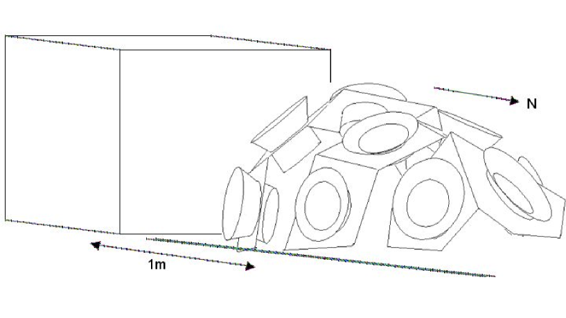
Figure 1: Schematic view of the PASS experiment, here drawn with ten cameras. The box in the background is the removable enclosure. An approximate size scale is indicated.

Driven by the requirement to obtain an all-sky transit survey on a reasonable operational timescale, a single PASS instrument would consist of an array of 15 CCD cameras of short focal length. With slightly overlapping fields the cameras would image the entire sky visible from an observing location. The CCD cameras would be unguided (Figs 1 and 2), thus ensuring excellent mechanical and photometric stability of the instrument. The instrument’s baseline design uses conventional read-out of the CCD chips, and stars would appear as trails in the images. Alternatively, the celestial motion parallel to a CCD’s columns may be compensated for by synchronous line-by-line read-out of the CCD. The current baseline consists of 15 cameras with lenses of $f=50$ mm, as used for common high quality SLR cameras (for 36mm film), with a CCD of appropriate size, of about 25 $\times$ 25 mm, which gives a field of view of about $28\arcdeg$ $\times$ $28\arcdeg$. Figure 2 shows that 15 such cameras would give complete coverage of the sky above an altitude of around 30$\arcdeg$. The experiment would need to be mounted on a sturdy platform and be covered by a completely removable enclosure. An important feature of the instrument will be the synchronization of the timing of the exposures with sidereal time (ST), such that images would always be taken at the same ST and, consequently, at the same set of hour angles. Hence, on different nights, but at the same ST, stars would trail over exactly the same CCD pixels, and images taken on one night would be directly comparable to images taken on other nights. This would allow relative photometry not only among groups of stars, but also among data sets from many nights. Systematic errors that do not vary from one night to another, such as flat-fielding errors, would therefore cancel out.

The amount of data produced would depend mainly on the size of the CCD chips (1k $\times$ 1k and 2k $\times$ 2k designs are being evaluated) and on the level of on-line processing being performed. If images are co-added (accounting for the stellar motion in the co-adding) and saved only every 500 s, about 800 images would be generated every night, each with a size of 2 Mbyte (for a 1k $\times$ 1k chip). This would result in fairly manageable data volumes of 1.6 Gbyte per night. Precession would cause a constant shifting of the star trails. This may be accounted for by an occasional recalibration of the tracks, or by mechanical adjustment, gradually turning the entire system around the precession axis.

4 Survey coverage

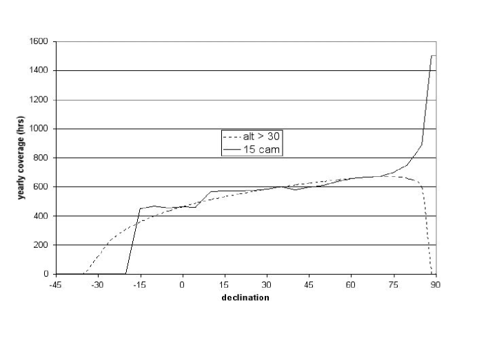
b)

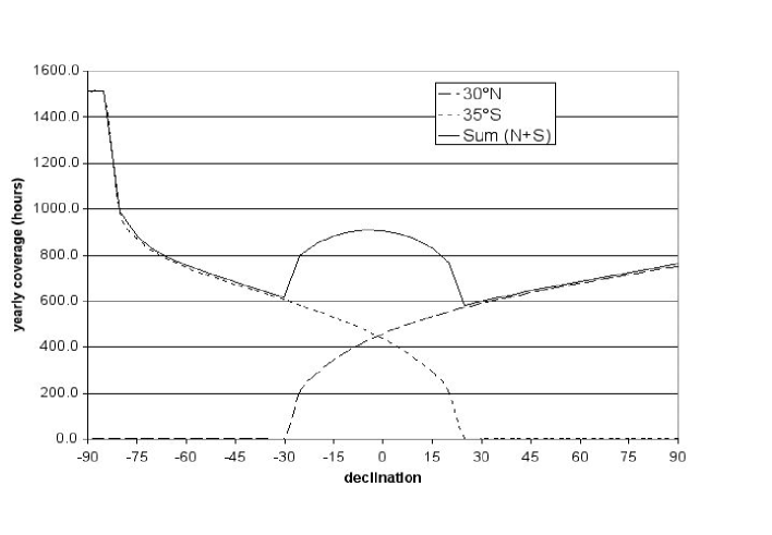
Figure 3: a) . Yearly observational coverage of dependence on stellar declination, assuming a yearly total of 1500 hours of clear observing conditions (200 nights of 7.5 hours) for a site at 28.5$\arcdeg$ N (Teide Observatory). The coverage shown here is the average for stars at any right ascension. Dashed line: Coverage if the entire sky above $30\arcdeg$ altitude is surveyed. The North Celestial Pole, at an elevation of $28.5\arcdeg$, is not covered. Solid line: coverage by the 15 camera system shown in Figure 2. A small region around the North Celestial Pole is now circumpolar by lowering the altitude limit to $27\arcdeg$ at very high northern declinations. b) As before, now showing temporal coverage from a northern ($30\arcdeg$ N) and southern ($35\arcdeg$ S) site, assuming simple $30\arcdeg$ altitude limits for both. If night hours do not overlap among the sites, coverage near the celestial equator will be the sum from both sites, and a relatively uniform coverage (solid line) of over 600 hr/yr is achieved over the entire sky.

The celestial sphere above an altitude of $30\arcdeg$ has a spatial angle of $1\pi$ sterad. Hence, a quarter of the entire sky will be observed at any time. The amount of time that a star can be observed during the course of a year depends primarily on its declination and on the observatory’s geographical latitude. Coverage also depends strongly on the lower limit for the altitude: For a $30\arcdeg$ altitude limit at a location at $30\arcdeg N$, the North Celestial Pole is permanently visible; stars at the stellar equator would be visible about 1/3 of the night annually, and coverage declines rapidly towards southern declinations (Fig. 3a). For the proposed camera configuration from a northern location ($30\arcdeg$ N) with a southern declination limit of $-$17.5$\arcdeg$ (Fig. 2), about 65% of the entire sky would be observable with a coverage of at least 400 hr/yr. The northernmost declination range might also be observed from an array that is located geographically farther north, which allows observing this part of the sky at lower airmasses. Coverage of southern declinations would be achieved from at least one instrument located in that hemisphere. This should preferably be located at a very different longitudes to avoid overlapping night hours. For stars near the celestial equator, the coverage from two observatories in antipodal positions could then be doubled (Fig. 3b), and an average coverage of at least 650 hr/yr could be achieved at any declination.

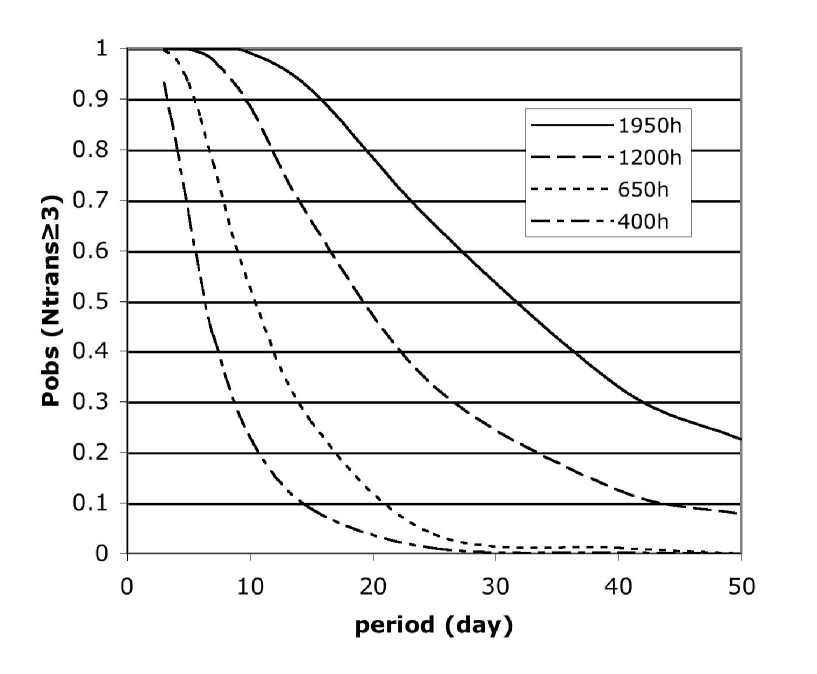
Figure 4: Probability, P_obs, that transiting planets will be detected, depending on their orbital period and observational coverage. The detection probability is based on the requirement to observe at least three transits. An observational coverage of 400 hours would be achieved from a single array at a mid-northern or mid-southern site (at about 30$\arcdeg$ N or S) during one year of observations (compare to Fig. 3), and 1200 hours during 3 years. 650 hours of observational coverage can be achieved in one year for stars at any declination from combined observations with a northern and southern array without overlapping night hours; 1950 hours corresponds to 3 years of observations with such a set-up.

For a reliable detection of planetary candidates, and in order to suppress false alarms from other sources (random high sigma events, or noise of instrumental, meteorological, or astronomical origin), observation of at least three transit events would be required. The probability of detecting a given number of transit events for a planet of given period is primarily dependent on the duration of the observational coverage. This calculation is given in Appendix A. Figure 4 shows the detection probability for observations for a duration of one and three years. In the latter case, coverages of at least 1200 hours should be achieved, thus allowing high (greater than 50%) detection probabilities for planets with orbital periods of up to 15 days. Longer observing spans would further increase the detectable orbital periods, increase the confidence in existing detections, and to some extent lower the detectable planet sizes owing to the observation of more transits.

A single array at a mid-northern or mid-southern (25–40$\arcdeg$ latitude) site could survey about 250 000 stars to $V=10.5$ mag with sufficient precision for the detection of giant planet transits (requiring photometry better then 0.35% in 900 s; see the following section). Similarly, a true all-sky survey could access about 400 000 stars. Following Brown (2003), only about 14% of bright field-stars are suitable for ground based transits searches (These are main-sequence stars with radii of less than 1.3R$\sun$). Assuming that about 1% of them have short-orbital giant planets (e.g., Udry et al. 2003), with a transit probability of 5%, about 20 planets may be detected from a 1-instrument survey, and 30 planets from an all-sky survey. It should be emphasized that the major goal of PASS is not the detection of large numbers of planets, but the complete detection of planets transiting bright stars within some well-established and consistent completeness limit.

5 Instrumental performance

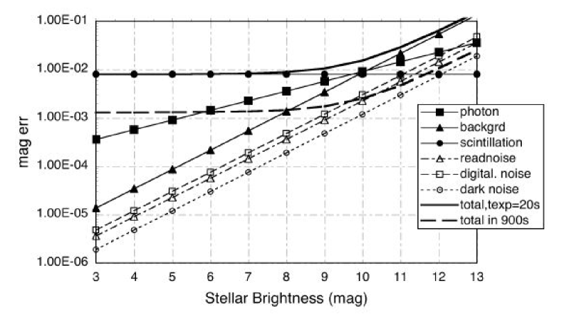
Figure 5: Noises of the PASS instrument against stellar magnitude, as expected in star-trail images. The thick dashed line is the total noise for 900 s integration, whereas all other lines indicate noises in a single 20 s exposure of a field at the celestial equator with the baseline set-up (see text). Photometric precision suitable for transit detection can be expected up to 10.5–11 mag. Stars brighter than 5.2 mag will be saturated.

It should be noted that star trail images have a different signal to noise (S/N) behavior than normal images with guided apertures. Whereas the S/N of guided aperture images increases with exposure time as $t_{\rm exp}^{1/2}$, the S/N of a single star trail image converges towards a fixed value for long exposure times. Consequently, in order to fill longer integrations, the acquisition and averaging of multiple shorter images is advantageous. An S/N equation describing this behavior is presented in Appendix B. Figure 5 shows the contribution from various noise sources that have been calculated for a baseline set-up of PASS. This consists of an $f=50$ mm lens operated at aperture $f$/2.0, with a red cut-off filter at 725 nm (to avoid atmospheric water lines), a front-illuminated CCD (1k $\times$ 1k size, 24 micron pixels, with a quantum efficiency of 0.46 against light from solar-type stars and 0.39 against light from sky background), resulting in system quantum efficiencies (which include the cut-off filter and an optical efficiency of 0.8) of 0.25 and 0.13 against stars and sky. Exposure times are 20 s, and for the baseline, observations of a field near the celestial equator ($\delta=0\arcdeg$) under a moonless sky at a dark site with 21.45 mag/arcsec² has been assumed (Benn & Ellison, 1998). Scintillation is calculated for 1.4 airmasses at an altitude of 2400 m, using the equation of Young (1974). Figure 5 shows that the three major noise sources are scintillation, photon noise from stellar sources, and photon noise from sky background. Other noises, all related to the CCD chip (read-out, dark signal, and digitization noise) are negligible. With stellar photon noise as the major noise source around 10th magnitude, the instrument may be considered as optimized for that magnitude range, with no significant improvements possible from the suppression of other types of noise.

The design of PASS, taking images from a fixed telescope and at fixed sidereal times will minimize any systematic errors. Photometric errors in guided telescopes arise from residuals in the flat-fielding correction under the slightly moving stellar point spread function, and from errors in the centering of the photometric aperture. Images taken by PASS will exhibit these same errors, but they will be identical in images taken at the same ST. The comparison of a star’s brightness against a group of reference stars in identical images from many nights will then cancel out these errors. This will leave second order errors. Temperature changes may affect the focussing, slightly varying the position of stellar images. One solution may be comparative photometry only within subsets of images taken at identical ST and at similar temperatures. Errors from seeing variations cannot be excluded either. However, they are not expected to be significant, since the resolution of the optical system and the angular size of the CCD pixels is much larger than any common seeing values. First order atmospheric extinction variations are cancelled out in any differential photometry among nearby stars. Since PASS fields are of very wide angle, the dependence of extinction on airmass needs careful monitoring, however. Second order wavelength dependent extinction variations may be minimized from an optimized selection of comparison stars. This implies that sample stars are classified according to their color into several groups, and that photometry is performed between stars of the same group. Since PASS will observe the same all-sky stellar sample over a long time, the creation of correction functions should be able to reduce most—if not all—of these errors. Such corrections can be expected to improve with prolonged observations, which implies the necessity to save all raw photometry of PASS for better re-reductions at later dates.

A limiting precision for transit detection may be defined from the requirement to detect transits with at least 1% brightness variation as 3-sigma signals in 900 s integrations. This corresponds to requiring a precision of at least 3.5 mmag over that integration time. For the baseline set-up, this leads to a survey limit of about 10.5 mag (see dashed line in Fig. 5). This may be considered a conservative limit, as transits last several hours and would produce numerous data points of 900 s integrations, leading to trains of 3-sigma signals that should readily be classifiable as transit candidates. A bright survey limit of about 5.5 mag is given by saturation of the CCD detector. The baseline set-up has been calculated for typical good observing conditions, as mentioned previously. Below, the limiting magnitudes for transit detection in different conditions are given (conditions marked * correspond to the baseline):

Moon: none*, gibbous, half moon, full moon:	10.5*,10.2, 9.7, 9.2
Apertures: $f$/1.4, $f$/1.8, $f$/2.0*:	11.0, 10.7, 10.5*
Exposure times: 5, 10, 20*, 30, 40, 50, 60, 100 sec	10.6, 10.6, 10.5*, 10.5, 10.4, 10.4, 10.3, 10.0
Airmass: 1.1, 1.4*, 1.7, 2.0:	10.6, 10.5*, 10.4, 10.2
Declination of sample field: 0$\arcdeg$*, 45$\arcdeg$, 60$\arcdeg$, 75$\arcdeg$, 89$\arcdeg$, 89$\arcdeg$ at 2 airmasses:
	10.5*, 10.6, 10.8, 11.1, 11.1, 10.6
Observatory altitude (m): 0, 1000, 2400*, 4000, 0 at 2 airmasses:      10.5, 10.5, 10.5*, 10.6,9.0
Back-illuminated CCD with higher QE of 0.66 for stars and 0.58 for sky:       10.7
CCD with double the resolution (12 $\mu$m pixels):	10.7

The last two entries show that the use of a back-illuminated—and significantly more expensive—CCD with higher quantum efficiency results in an increase in limiting magnitude of only 0.2 mag. Also, the use of CCDs with double the spatial resolution would lead only to small gains, mainly from the inclusion of smaller areas of sky-background within stellar apertures. The signal-to-noise calculations therefore give confidence that the objective of the experiment can be reached with the baseline design, that objective being maintained in a variety of differing conditions. It should be noted that the above mangitude limits are for an expected “typical” planetary transit. Lower magitude limits may be achieved for larger ($\gtrsim 1.2\ R_{\rm Jup}$) planets and for many studies not related to planet detection, as listed in Section 2.

6 Photometry on simulated images

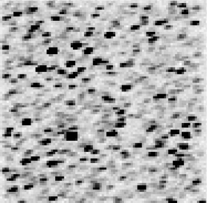
a)b)

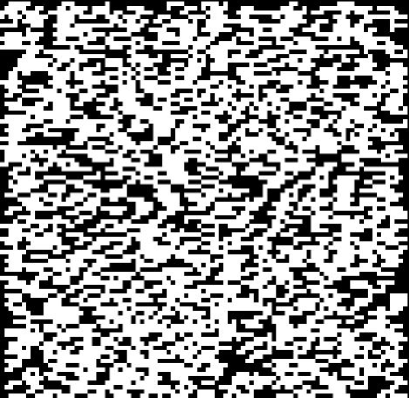
Figure 6: a) Simulated PASS image (with stellar density typical for 10$\arcdeg$ galactic latitude), with an exposure of 20 s and the baseline set-up. The size of the field is about 2$\arcdeg$ $\times$ 2$\arcdeg$. The brightest star has 5.7 mag, several have 6–9 mag, and the faintest ones are 14–15 mag. b) Final aperture mask. Starting from the brightest stars, the maximum number of non-overlapping traces has been fitted in (here extracting apertures for 1155 stars), so that each aperture pixel (white) is assigned to just one star.

A simulator for CCD images by PASS has been developed to evaluate if the noise sources predicted in the previous section can be corrected for by photometry done on realistic images. Besides the noise sources described previously, the simulations also represent stellar crowding and the variations in inter-pixel quantum efficiency expected in front-illuminated CCDs, as described by Kavaldjiev & Ninkov (1998). Figure 6a shows a simulated field that represents a small fraction of the field size that would be observed by one of PASS’s cameras, with a simulated stellar density typical for galactic latitudes of 10$\arcdeg$ (Allen, 1973; Cox, 1999). Sequences of such images have been generated in the simulations, regenerating the appropriate noises every time and optionally accounting for the motion of the stars from field to field. Stellar photometry is being performed on these image sequences with a program tracephot, written in IDL. In its first analysis step, an aperture mask is built up on the first image, based on known stellar positions and brightnesses (from the input catalog), using the following method. The program starts with the brightest star and assigns any pixels under its trail to that star’s aperture. This process is continued for fainter and fainter stars, but stars part of whose trails are already assigned to brighter stars are rejected. With this algorithm, the maximum number of the brightest stars is sampled in the field, resulting in very dense final aperture masks similar to those shown in Figure 6b. The crowding encountered in the $b$ = 10$\arcdeg$ sample field and expressed as the fraction of confused apertures against stellar brightness is indicated in Table 1. There, Nstars is the number of stars that were in the simulation’s input catalog. Nassign is the number of stars for which apertures could be assigned and photometry extracted, and Nconfused is the number of confused and hence irretrievable stars, with frac_conf being the fraction of confused stars. Only for magnitudes fainter than $\approx$ 12 are a significant fraction of stars rejected due to confusion. In the second step, tracephot applies the aperture mask to the first image and then, with appropriate shifts, to the following ones. Simple aperture photometry is then performed through these masks, resulting in a time-series for each star. The major factor that can be expected to degrade the observed photometric precision against the theoretical one, especially among the fainter stars, is caused by the crowding that many of these stars are suffering. Although the aperture assignment algorithm ensures that the largest fraction of light in each pixel in a given stellar aperture comes from the star being measured, it cannot preclude a significant fraction of light coming from other, fainter stars, which will result in additional noise. Figure 7 shows the rms error of photometry of such a time-series from the baseline set-up, against the known input brightness of the stars. Comparison with the theoretical noise figures (solid line in Fig. 5) shows that the photometry on stellar traces is able to extract brightnesses for most stars with noise types intrinsic to the images.

7 Conclusions and outlook

An experiment for the detection of transiting planetary systems around all bright stars in the entire sky is described, within magnitudes of about 5.5 – 10.5. The instrument would also provide the starting point for permanent photometric tracking of variable stars of any kind.

The field of transit detection has reached a point of inflection, where it becomes obvious that previous estimates of the discovery rates of transiting planets are turning out to be too optimistic. For example, Horne (2003) predicted for the current transit experiments a total of 10 to 100 planet detections per month, and cites six monthly detections for PASS and two monthly detections for the STARE project. This latter has been in regular operation since 2001, but to date only one transiting planet has been discovered (Alonso et al., 2004a). For PASS, our estimate gives a total of 30 detected hot giant planets with a single array (Section 4), which might be achieved after 3–4 years of continuous operation, corresponding to an average monthly detection rate of about one planet. This discrepancy probably results from several factors: simplifying assumptions in the noise characteristics that governed detection limits in previous predictions (in particular unaccounted errors in aperture photometry on guided telescopes), overestimates of the fraction of stars that are suitable as targets for transit surveys, and underestimates of the required observational coverage. Large amounts of transit-like events can be quickly found by any detection experiment (one of the few published data at that stage are the transit-candidates from OGLE, Udalski et al. 2002a, b). The first cut in the selection of “good” candidates (i.e., those worth detailed follow-up) is to seek periodicity, which needs the observation of at least three transit events. Even for short-period hot giants, however, this requires at least 300–400 hours of observations to achieve detection probabilities $>$ 0.5, which corresponds to observing for at least 50 nights (see Fig. 4 and Appendix A). Many attempts with shorter coverage have indeed failed to produce any reliable detections, a typical example being Street et al. (2003). We do not wish to imply that these earlier predictions or observational attempts were in any way faulty, but they do show that the field has matured through the experience gained in the course of several campaigns. It is also becoming clear that the detection of a transit is only the first link in a chain to produce reliable planet detections. Estimates by Brown (2003) show that a large fraction of—if not most—transit-like events in giant planet searches will be produced by several stellar configurations with eclipsing binaries. Based on the experience from STARE, Alonso et al. (2004b) propose a staged approach at false alarm detection: It begins with a careful review of the transit parameters following the precepts by Seager & Mallén-Ornelas (2003), and is followed by observations that are simple and progress towards more demanding observations. These start with transit observations in several different colors, which will eliminate most eclipsing binaries, and finalize in radial velocity measurements that may lead to an independent verification of a planet. The brightness of the sample surveyed by PASS will greatly facilitate such observations, making first verification observations possible even from rather small 20–30 cm class telescopes. Radial velocity measurements should not cause significant difficulties, either. Still, the large sample size of PASS will need a well-coordinated effort for follow-up observations, and help from the amateur community might play a very useful role for some verification observations.

In this first paper, the basic set-up, S/N considerations, and simulations are described that indicate that the baseline design of the instrument could indeed fulfill the main objective. Finance has been obtained for the placement of a prototype system. This system comprises two CCD cameras with 50 mm Nikon lenses, with an initial location at Teide Observatory on Tenerife, where a small dome is currently being constructed. It is described in more detail in Deeg et al. (2004). The principal goal of the prototype is the undertaking of a feasibility study, for which measurements under a variety of observing conditions and pointings will be obtained. The prototype will also allow refinement of observing strategies and deliver real data that will aid in the development and testing of the future reduction pipeline. Once these observations have finished, it is envisaged to point the two cameras to about 62$\arcdeg$ declination and hour-angles of + and - 1h 20 min (+ and - 20 $\arcdeg$ in Fig. 2), thereby starting the first operating elements of PASS.

8 Acknowledgement

The authors are grateful to the referee, whose comments led to a clearer discussion in parts of this paper. Part of this project is being funded by grant AYA-2002-04566 of the Spanish Ministerio de Educación y Ciencia.

Appendix A Probability of observing a required number of transits

The following calculation gives the probability that at least $N_{\rm tr}$ transits of a transiting system are being observed, in observations spanning a time $T_{\rm obs}$, during which a fraction $f_{\rm cov}$ of temporal coverage is achieved (thereby giving an observational coverage of $T_{\rm cov}=T_{\rm obs}f_{\rm cov}$). For a transiting planet with period $P$, the probability, $p_{\rm tr}$, of observing at least part of a transit with observations lasting for one period ($T_{\rm obs}=P$) is given by

$$p_{\rm tr}=\frac{(\mbox{time observed within }P)}{P}=f_{\rm cov};$$ (A1)

e.g., $p_{\rm tr}$ is identical to the duty cycle, $f_{\rm cov}$. The probability of missing the transit is $p_{\rm notr}=1-f_{\rm cov}$. For multiple transits, the probability of observing exactly $k$ transits within a time $T_{\rm obs}=n\cdot P$ is then represented by the binominal distribution:

$$p_{k{\rm{~{}transits~{}in~{}}}{\rm time}n\cdot P} = {n\choose k}p_{\rm tr}^{k}p_{\rm notr}^{n-k}$$ (A2)

$$= {n\choose k}f_{\rm cov}^{k}(1-f_{\rm cov})^{n-k},$$

where ${n\choose k}$ is the number of combinations of $k$ in $n$ without repetition. The probability to observe at least $N_{\rm min}$ transits during is then given by the summation over above terms:

$$p_{N_{\rm tr}\geq N_{\rm min}}=\sum_{k=N_{\rm min}}^{n}p_{k}=1-\sum_{k=0}^{N_{\rm min}-1}p_{k}.$$ (A3)

The above equations are correct so long as the number of periods within the observations, $n=T_{\rm obs}/{P}$, is slightly larger than $N_{\rm min}$. For $n-N_{\rm min}\lesssim 5$, or duty cycles $f_{\rm cov}$ approaching 1, the detection probabilities are dominated by aliasing effects.

A further simplification is possible for low duty cycles, $f_{\rm cov}$, and large $n$ where we can use the relation (e.g., Bronstein & Semendjajew 1979)

$$p_{k}={n\choose k}p^{k}{q}^{n-k}=\frac{\lambda^{k}}{k!}e^{-\lambda},$$ (A4)

where $q=1-p$ and $\lambda=np$. Replacing $n$ by $T_{\rm obs}/{P}=T_{\rm cov}{(f_{\rm cov})}P$, and $p$ by $p_{tr}=f_{cov}$ (hence, $\lambda=T_{\rm cov}/P$) gives:

$$p_{k}=\frac{(T_{\rm cov}/P)^{k}}{k!}\ e^{-T_{\rm cov}/P}.$$ (A5)

.

The detection probability, $p_{N_{\rm tr}\geq N_{\rm min}}$, can then be obtained by a summation similar to the previous one. It should be noted that this equation is independent of $f_{cov}$ and in practice gives good results so long as $f_{\rm cov}\lesssim 0.5$.

Appendix B Signal-to-noise equation for trailing star images

In the equation to be derived, we consider only the noises dominated by photon statistics, from the stellar source, and the sky background. Similarly for normal stellar images with guided apertures, the S/N is then given by

$$S/N=N_{\rm ph,*}/\sqrt{N_{\rm ph,*}+N_{\rm ph,s}},$$ (B1)

where $N_{\rm ph,*}$ and $N_{\rm ph,s}$ are the count of detected photons from star and sky in a given aperture. The photon count from a star in a time $t$ may be expressed by its flux as

$$N_{\rm ph,*}=\phi_{*}t.$$ (B2)

For the photon count detected from sky-background, in trailing star images the increase of the aperture with time has to be taken into account. If $\phi_{\rm s}$ denotes the sky-flux per area in the detector-plane, then

$$N_{\rm ph,s}=\phi_{\rm s}tA(t),$$ (B3)

where $A(t)$ is the area of the aperture, which may be given by $A(t)=D^{2}\pi/4+D\omega t$, where $D$ is both the focal-plane aperture diameter for very short exposures and the width of a trail-shaped aperture for longer exposures, and $\omega$ is the velocity of a stellar image across the detector, given by: $\omega=2\pi f(\cos\delta)/1Sd$, where $f$ is the focal length, $\delta$ the star’s declination, and $1Sd$ = 86164 s is the length of a sidereal day. Hence,

$$N_{\rm ph,s}=\phi_{\rm s}(D^{2}\pi/4t+D\omega t^{2}).$$ (B4)

Inserting this into the first equation, the S/N equation for single trailing star images is then obtained:

$$S/N=\frac{\phi_{*}t}{\sqrt{t(\phi_{*}+\phi_{\rm s}D^{2}\pi/4)+t^{2}\phi_{\rm s}D\omega}}$$ (B5)

For long exposures the $t^{2}$ term dominates, and S/N converges towards

$$S/N_{t\to\infty}=\frac{\phi_{*}}{\sqrt{\phi_{\rm s}D\omega}}.$$ (B6)

Long integration times are therefore better filled with multiple shorter individual exposures. If the noise of single images is dominated by Poisson statistics, then their measurements can be averaged, and the combined S/N for $n$ images increases by $n^{1/2}$. For an integration time of $t_{\rm int}$, which is filled by $n=t_{\rm int}/(t+t_{\rm dead})$ images, where $t_{\rm dead}$ is the ’dead-time’ lost between exposures, the S/N is then given by:

$$S/N_{t_{\rm int}}=\left({\frac{t_{\rm int}}{t+t_{\rm dead}}}\right)^{1/2}\>\frac{\phi_{*}t}{\sqrt{t(\phi_{*}+\phi_{\rm s}D^{2}\pi/4)+t^{2}\phi_{\rm s}D\omega}}$$ (B7)

Fig. 8 shows the behaviour of this equation for varying values of exposure time $t$ for the PASS project, with a dead-time of $t_{\rm dead}=4$sec. For trailing star observations with a finite dead-time between exposures, there exists an optimum exposure time for single images that allows the filling of any long integration by sequences of shorter images. For applications such as that presented here with the PASS project, with several further noise sources beyond photon noise from stars and sky, the quantity $t_{\rm opt}$ is most conventiently determined by calculating the S/N as shown in Fig. 7 with varying values of $t$. For the PASS baseline, assuming a CCD read-out time of 4 s, an exposure time of about 13 s optimizes S/N for stars of mag 11 at equatorial regions, whereas 26 seconds are optimum for declinations of 60$\arcdeg$. Since the relation of S/N to $t$ has a very broad peak, a uniform exposure time of 20 s has been assumed for the baseline, with losses of not more than 0.1 mag in limiting magnitudes at any declination.

Figure 2: Local all-sky view from a location at 28.5$\arcdeg$ N, showing camera positions (squares) for a system of 15 units (each with a field of view of 28$\arcdeg$ $\times$ 28$\arcdeg$), in orthogonal projection. Coordinate lines are declination and hour angle; also indicated is an altitude of 30$\arcdeg$ (long dashes around circumference). In this set-up, there is no coverage below declinations of $-$17.5$\arcdeg$, as good temporal coverage of stars further south cannot be obtained (see Fig. 3a). Further north, the sky is completely covered for altitudes $>34\arcdeg$ with an average limit around 30$\arcdeg$. The altitude limit is slightly lowered in the extreme north, to include the North Celestial Pole. Other camera positionings have been evaluated, but for a view of 28$\arcdeg$ this is the most efficient one.

a)

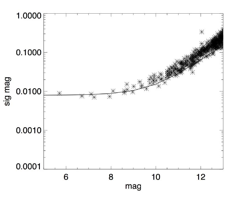
Figure 7: Crosses indicate the rms error found in time-series photometry on the artificial stars in 15 simulated images similar to those shown in Figure 6a. The solid line is identical to the uppermost solid line in Fig. 5 and indicates the total expected noise from S/N calculations. Some stars have photometric errors “better” than the theoretical value; this is a result of the small sample of only 15 images.

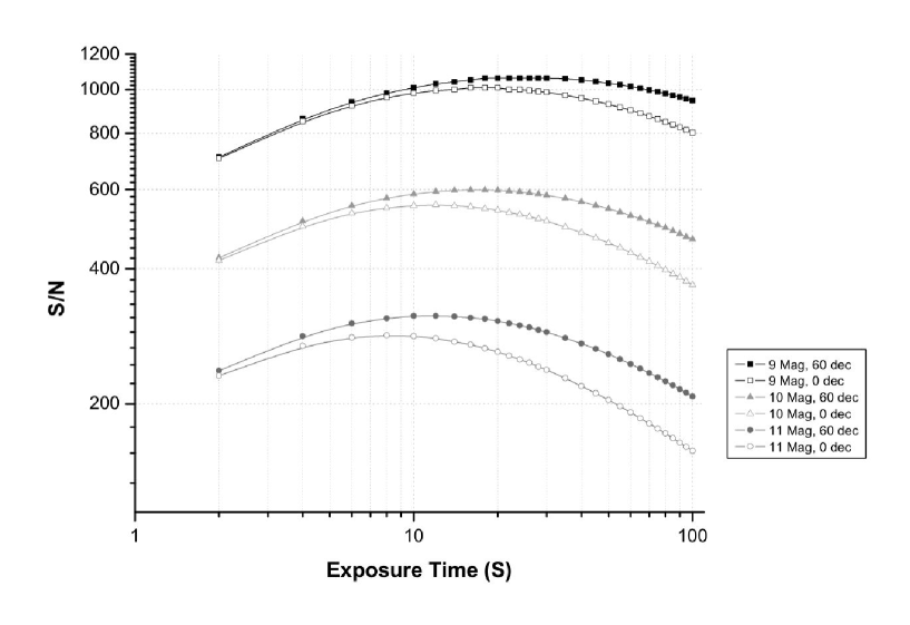
Figure 8: Dependency of the signal-to-noise of a long integration on the exposure time of individual star-trail images, as given by Eq. (B7). In the graph, an integration time of 900 second is assumed, and S/N is shown at declinations of 0$\arcdeg$ and 60$\arcdeg$and for stars with magnitudes of 9, 10 and 11. The difference in S/N with declination comes from the varying velocity of the stars across the detector. Only the photon noise from star and sky-background is considered here, using values from the ’PASS-baseline’

Table 1: Crowding in PASS field at $l=10\arcdeg$ and fraction of confused apertures

mag	Nstar	Nassign	Nconfused	fracconf
4.5–5.5	1	1	0	0.000
5.5–6.5	1	1	0	0.000
6.5–7.5	3	2	1	0.333
7.5–8.5	3	3	0	0.000
8.5–9.5	9	9	0	0.000
9.5–10.5	19	18	1	0.053
10.5–11.5	76	71	5	0.066
11.5–12.5	163	132	31	0.190
12.5–13.5	462	283	179	0.387
13.5–14.5	1099	334	765	0.696
14.5–15.5	2383	301	2082	0.874

References

- Allen (1973) Allen, C. 1973, Astrophysical Quantities (London: Athlone Press)
- Alonso et al. (2004a) Alonso, R., Brown, T., Torres, G., Latham, D., Sozzett, A., Belmonte, J., Charbonneau, D., Deeg, H., Dunham, E., Mandushev, G., O’Donovan, F., & Stefanik, R. 2004a, submitted to ApJL
- Alonso et al. (2004b) Alonso, R., Deeg, H. J., Brown, T. M., & Belmonte, J. A. 2004b, submitted to Astronomische Nachrichten
- Benn & Ellison (1998) Benn, C. R., & Ellison, S. L. 1998, La Palma Tech. Note 115, Tech. rep., Isaac Newton Group of Telescopes, La Palma
- Bouchy et al. (2004) Bouchy, F., Pont, F., Santos, N. C., Melo, C., Mayor, M., Queloz, D., & Udry, S. 2004, A&A, 421, L13
- Bronstein & Semendjajew (1979) Bronstein, I., & Semendjajew, K. 1979, Taschenbuch der Mathematik (Thun, Frankfurt/Main: Verlag Harri Deutsch), 701
- Brown (2003) Brown, T. M. 2003, ApJ, 593, L125
- Caldwell et al. (2003) Caldwell, D. A., Witteborn, F. C., Showen, R. L., Ninkov, Z., Martin, K. R., Doyle, L. R., & Borucki, W. J. 2003, Astronomy in Antarctica, 25th meeting of the IAU, Special Session 2, 18 July, 2003 in Sydney, Australia, 2
- Charbonneau (2003) Charbonneau, D. 2003, in ASP Conf. Ser. 294, Scientific Frontiers in Research on Extrasolar Planets, eds. D. Deming, S. Seager (San Francisco: ASP), 449
- Charbonneau et al. (2000) Charbonneau, D., Brown, T. M., Latham, D. W., & Mayor, M. 2000, ApJL, 529, L45
- Charbonneau et al. (2002) Charbonneau, D., Brown, T. M., Noyes, R. W., & Gilliland, R. L. 2002, ApJ, 568, 377
- Cox (1999) Cox, A., ed. 1999, Allen’s Astrophysical Quantities (Springer, AIP press)
- Deeg et al. (2004) Deeg, H., Alonso, R., Belmonte, J., Horne, K., Alsubai, K., & Doyle, L. 2004, Astronomische Nachrichten, 325, in print
- Deeg (2002) Deeg, H. J. 2002, in Proceedings of the First Eddington Workshop on Stellar Structure and Habitable Planet Finding, 11 - 15 June 2001, Cordoba, Spain. Editor: B. Battrick, Scientific editors: F. Favata, I. W. Roxburgh, D. Galadi. ESA SP-485, (Noordwijk: ESA Publications Division), 273
- Henry et al. (2000) Henry, G. W., Marcy, G. W., Butler, R. P., & Vogt, S. S. 2000, ApJ, 529, L41
- Horne (2003) Horne, K. 2003, in ASP Conf. Ser. 294, Scientific Frontiers in Research on Extrasolar Planets, eds. D. Deming, S. Seager (San Francisco: ASP), 361
- Kavaldjiev & Ninkov (1998) Kavaldjiev, D., & Ninkov, Z. 1998, Optical Engineering, 37, 948
- Konacki et al. (2003a) Konacki, M., Torres, G., Jha, S., & Sasselov, D. D. 2003a, Nature, 421, 507
- Konacki et al. (2003b) Konacki, M., Torres, G., Sasselov, D. D., & Jha, S. 2003b, ApJ, 597, 1076
- Konacki et al. (2004) Konacki, M., Torres, G., Sasselov, D. D., Pietrzyński, G., Udalski, A., Jha, S., Ruiz, M. T., Gieren, W., & Minniti, D. 2004, ApJ, 609, L37
- Pepper et al. (2003) Pepper, J., Gould, A., & Depoy, D. L. 2003, Acta Astronomica, 53, 213
- Pepper et al. (2004) Pepper, J., Gould, A., & DePoy, D. L. 2004, ArXiv Astrophysics e-prints
- Pojmański (2001) Pojmański, G. 2001, in ASP Conf. Ser. 246: IAU Colloq. 183: Small Telescope Astronomy on Global Scales, eds. W.-P. Chen, C. Lemme, B. Paczynski, 53
- Seager & Mallén-Ornelas (2003) Seager, S., & Mallén-Ornelas, G. 2003, ApJ, 585, 1038
- Seagroves et al. (2003) Seagroves, S., Harker, J., Laughlin, G., Lacy, J., & Castellano, T. 2003, PASP, 115, 1355
- Street et al. (2003) Street, R. A., Horne, K., Lister, T. A., Penny, A. J., Tsapras, Y., Quirrenbach, A., Safizadeh, N., Mitchell, D., Cooke, J., & Cameron, A. C. 2003, MNRAS, 340, 1287
- Udalski et al. (2002a) Udalski, A., Paczynski, B., Zebrun, K., Szymaski, M., Kubiak, M., Soszynski, I., Szewczyk, O., Wyrzykowski, L., & Pietrzynski, G. 2002a, Acta Astronomica, 52, 1
- Udalski et al. (2003) Udalski, A., Pietrzynski, G., Szymanski, M., Kubiak, M., Zebrun, K., Soszynski, I., Szewczyk, O., & Wyrzykowski, L. 2003, Acta Astronomica, 53, 133
- Udalski et al. (2002b) Udalski, A., Zebrun, K., Szymanski, M., Kubiak, M., Soszynski, I., Szewczyk, O., Wyrzykowski, L., & Pietrzynski, G. 2002b, Acta Astronomica, 52, 115
- Udry et al. (2003) Udry, S., Mayor, M., & Queloz, D. 2003, in ASP Conf. Ser. 294, Scientific Frontiers in Research on Extrasolar Planets, eds. D. Deming, S. Seager (San Francisco: ASP), 17
- Vestrand et al. (2002) Vestrand, W. T., Borozdin, K. N., Brumby, S. P., Casperson, D. E., Fenimore, E. E., Galassi, M. C., McGowan, K., Perkins, S. J., Priedhorsky, W. C., Starr, D., White, R., Wozniak, P., & Wren, J. A. 2002, in Proc. SPIE, 4845, 126
- Young (1974) Young, A. 1974, in Methods of Experimental Physics, Vol. 12, Astrophysics, Part A, ed. N. Carleton (New York: Academic)