Tunable-filter imaging of quasar fields at $z\sim 1$. II. The star-forming galaxy environments of radio-loud quasars

Abstract

We have scanned the fields of six radio-loud quasars using the Taurus Tunable Filter to detect redshifted [O ii] $\lambda 3727$ line-emitting galaxies at redshifts $0.8<z<1.3$. Forty-seven new emission-line galaxy (ELG) candidates are found. This number corresponds to an average space density about $100$ times that found locally and, at $L$([O ii]) $<10^{42}$ erg s^-1 cm^-2, is $2-5$ times greater than the field ELG density at similar redshifts, implying that radio-loud quasars inhabit sites of above-average star formation activity. The implied star-formation rates are consistent with surveys of field galaxies at $z\sim 1$. However, the variation in candidate density between fields is large and indicative of a range of environments, from the field to rich clusters. The ELG candidates also cluster — both spatially and in terms of velocity — about the radio sources. In fields known to contain rich galaxy clusters, the ELGs lie at the edges and outside the concentrated cores of red, evolved galaxies, consistent with the morphology-density relation seen in low-redshift clusters. This work, combined with other studies, suggests that the ELG environments of powerful AGN look very much the same from moderate to high redshifts, i.e. $0.8<z<4$.

1. Introduction

Tracing star formation over the history of the universe is crucial for understanding the creation and evolution of galaxies. In global terms, the integrated star formation rate (SFR) per unit volume was at its peak at $z\sim 1$ (eg: Ellis et al. 1996; Lilly et al. 1996; Madau et al. 1996; Madau, Pozzetti & Dickinson 1998 but see Cowie, Songaila & Barger 1999). However, the physical explanation for such strong redshift dependence is still under question. In hierarchical models, $z\sim 1$ should also be an epoch of major galaxy-cluster assembly, with numerous mergers and subcluster development (eg: Lacey & Cole 1993; Khochfar & Burkert 2001; Murali et al. 2002). The fraction of blue galaxies in clusters at $z=1$ is higher than in similar systems at $z=0$ (Butcher & Oemler, 1984; Dressler & Gunn, 1992) and some studies suggest that star formation is suppressed in the centres of galaxy clusters relative to the field, at least out to $z\sim 0.5$ (Balogh et al., 1997, 1998). Furthermore, the cores of galaxy clusters may show a deficit of active galactic nuclei (AGN) as well as strongly star-forming galaxies (Barr et al. 2003; Miller & Owen 2003). The space density of AGN also peaks at high redshift and declines after $z\sim 1$ (eg: Boyle & Terlevich 1998). So, environment may strongly influence both star formation and AGN activity.

Magnitude-limited, spectroscopic field and cluster samples of strongly star-forming emission-line galaxies (ELGs) become incomplete by $z\sim 1$. At this redshift and beyond, narrow-band imaging techniques are more efficient at detecting ELGs. Narrow-band searches have a major advantage over magnitude-limited surveys in that they select objects directly on the basis of their star formation activity. At $z\sim 1$, ELGs typically have very faint continuum magnitudes, $I\gtrsim 21$ (Cowie et al., 1997; Cardiel et al., 2003), and are unremarkable in broad-band images – if seen at all. Indeed, studies have shown that magnitude-limited surveys can miss a substantial amount of star formation even at $z=0.4$ (Jones & Bland-Hawthorn 2001; hereafter JBH01). To cover the large volumes needed for surveys of star-forming galaxies at moderate to high redshifts, tunable-filter instruments offer an advantage over traditional monolithic filters in being able to target a wide range of wavelengths in contiguous passbands.

This paper presents tunable-filter observations designed to detect ELGs in the fields of six radio-loud quasars at $z\sim 1$ to investigate the links between AGN activity, environment and star formation at redshifts where AGN, star and structure formation all peak. Powerful AGN — particularly radio-loud AGN — are known to inhabit regions of above-average galaxy density (Yee & Green 1984; Ellingson et al. 1991; Wold et al. 2000; Pentericci et al. 2000; McLure & Dunlop 2001; Venemans et al. 2002; Barr et al. 2003) , and may even trace the first overdense regions to collapse. ELGs in some AGN fields have been detected with narrow-band imaging using monolithic filters (Pentericci et al. 2000; Hall et al. 2001; Kurk et al. 2001; Venemans et al. 2002), but to date systematic searches of homogeneous samples, as is possible with tunable filters, have not been carried out.

In this work, we target the redshifted [O ii] $\lambda 3727$ emission line. The [O ii] line has the benefit of being in the optical regime out to $z\sim 1.5$ and has been used widely as an empirically calibrated measure of star formation rate (SFR) (eg: Hutchings, Crampton & Persram 1993; Hammer et al. 1997; Kennicutt 1998; Hogg et al. 1998; Gallego et al. 2002; Hicks et al. 2002). Although a more direct SFR indicator, H$\alpha$ is only visible in the infrared at $z>0.5$. Also, [O ii] is not as susceptible to dust or resonant scattering effects as, for example, the Ly$\alpha$ line.

The Taurus Tunable Filter (TTF) etalon on the Taurus-2 instrument at the Anglo-Australian Telescope (AAT) provides a Fabry-Perot-based imaging system which allows high-efficiency, narrow-band imaging over a range in wavelength. Spectral resolutions, $\approx 100-1000$ are attainable from 3700Å to 10000Å (Bland-Hawthorn & Jones 1998a, 1998b). With its high throughput and narrow bands, TTF can achieve sensitivities of $\sim 10^{-17}$ erg s^-1 cm^-2 arcsec^-2 ($3\sigma$) in 12 minutes of integration. This is sufficient to probe [O ii] emission in galaxies with star formation rates greater than a few M_⊙ yr^-1 at $z\sim 1$.

Baker et al. (2001; hereafter Paper 1) demonstrated that it is possible to target [O ii] emission from star-forming galaxies around a quasar at $z=0.898$ using the TTF. We now use this instrument to examine the fields of a small sample of six additional quasars at $0.8<z<1.3$ for [O ii] emission. Target field selection and observing techniques are outlined in §2. The detailed procedure for reducing these observations is described in §3, and results are presented in §4. Implications are discussed in §5.

For a full discussion of the TTF and its use in finding emission-line galaxies, the reader is encouraged to consult JBH01, Paper 1 or Jones, Shopbell & Bland-Hawthorn (2002; J02). The data reduction presented here is as described in Paper 1, while the ELG selection algorithm is that of J02. We adopt an $H_{0}=70$ km s^-1 Mpc^-1, $\Omega_{\Lambda}=0.7$, flat-universe cosmology. Where results of Paper 1 are incorporated, they are adjusted to these values.

2. Observations

2.1. Target selection

Targets are drawn from the Molonglo Quasar Sample (MQS; Kapahi et al. 1998) of low-frequency-selected RLQs. This is a highly complete ($>97\%$) sample of 111 RLQs with $S_{408}>0.95$ Jy in the declination range $-30^{\circ}<\delta<-20^{\circ}$, and Galactic latitude $|b|>20^{\circ}$ (excluding the R.A. ranges $06^{\mathrm{h}}00^{\mathrm{m}}$ – $09^{\mathrm{h}}00^{\mathrm{m}}$ and $14^{\mathrm{h}}03^{\mathrm{m}}$ – $20^{\mathrm{h}}20^{\mathrm{m}}$). These quasars are, on average, five times less powerful and so considerably more numerous at a given redshift than the rarer 3CR sources (Laing, Riley & Longair 1983).

The six quasars whose fields are targetted in this work are listed in Table 1 and were chosen from the MQS parent sample purely according to criteria of observability. Suitable redshifts are limited by the need to place [O ii] inside the wavelength ranges accessible through the set of $\sim 200$Å-wide TTF order-blocking filters. Additional constraints were solely due to RAs and weather-affected runs, so the final list is a representative selection. We emphasise that no preselection was invoked regarding the likelihood of observing a cluster about a particular source.

The sample is chosen to be matched in radio power and therefore the variance in this property is small, covering less than one decade. It is therefore difficult to draw conclusions regarding the correlation between the properties of the quasars or their environments, and radio luminosity. We do not undertake any analysis of this type. It is noted, however, that studies comparing clustering in the environments of RLQs with their radio-quiet counterparts generally find that the locales of each type of quasar are indistinguishable Wold et al. (2000, 2001); Finn, Impey, & Hooper (2001); McLure & Dunlop (2001).

Table 1TTF targets and instrument parameters.

Run	MRC	Obs.	$z$	$\lambda$([O ii])	Blocking	Bandpass	Exposure	Seeing	Standard
	quasar	Date			Filter	FWHM	time		Star
				(Å)	(Å)	(Å)	(s)	(′′)
(1)	(2)	(3)	(4)	(5)	(6)	(7)	(8)	(9)	(10)
A	B0106–233	1999-Sep-07	0.818	6776	6680/210	10.5	10500	1.7	LTT 1020
B	B0413–210	1997-Oct-23	0.807	6735	6680/210	14.0	7000	0.9	LTT 1788
C	B1359–281	2000-Jul-29	0.802	6716	6680/210	10.2	8400	1.4	LTT 6248
D	B2021–208	2000-Jul-29	1.299	8568	8570/400	15.0	16800	1.1	LDS 749B
E	B2037–234	1999-Sep-07	1.150	8013	8140/330	15.4	14000	1.5	LTT 7987
F	B2156–245	1997-Oct-23	0.862	6940	7070/260	11.6	7000	0.9	LTT 9239

Note. — (1) run ID; (2) object name; (3) observation date; (4) redshift; (5) redshifted [O ii]; (6) TTF blocking filter central wavelength/bandpass; (7) TTF scan bandpass; (8) total exposure time; (9) average seeing; (10) standard star used to calibrate the observation.

Paper 1 reported TTF observations of the field of one MQS quasar, MRC B0450–221, the first RLQ observed in our program to image ELGs in the environments of RLQs. The reader is referred to this paper for details of the observations and data reduction. Results from the examination of ELG candidates in the field of MRC B0450–221 will be incorporated into the discussion of the collected properties of ELG candidates in the fields of quasars (§5).

2.2. Instrumental setup

Observations of the MQS targets in this work were made using TTF at f/8 on the AAT on 1997 October 23, 1999 September 7 and 2000 July 29. In each instance the MITLL2 CCD was windowed and masked to give a $9^{\prime}\!\!.87$ diameter circular field with a pixel scale of $0^{\prime\prime}\!\!.37$.

TTF scanned the quasar fields at seven plate spacings, $Z$ ($\propto\lambda$), corresponding to a series of steps of $\sim 10$Å either side of, and centred on, the redshifted [O ii] line. The transmission profiles of the blocking filters and individual TTF scans are shown in Figure 1 for each run. For run F, the blocking filter was tilted by $12^{\circ}$ in order to push the sensitivity $\sim 100$Å blueward. At each plate spacing, $2-4$ images were taken in a non-repeating pattern, with a relative spatial offset of $\sim 10^{\prime\prime}$ on the sky, to facilitate the removal of cosmic rays, bad pixels and ghost images.

Figure 1.— Passband sampling used in the TTF observations (profiles approximated by Gaussians: solid lines). The wavelengths shown are as measured at the location of the quasar near the field centre (note the wavelength sampled varies radially across the field for a given observation: see text). The transmission profiles of the order-blocking filters are shown as dashed lines. In the case of MRC B2156–245, the $R1$ blocking filter has been tilted by $12^{\circ}$ in order to push its sensitivity $\sim 100$Å blueward. The FWHMs and steps are given in Å.

Fabry-Perot imagers have a quadratic radial wavelength dependence ($\lambda\propto r^{2}$); for the etalon tilts used in this study the wavelength sensitivity varies across the field by 10 – 20Å. Figure 2 shows this variation for the field of MRC B2021–208, as well as a ‘night-sky ring’, caused by the radial sensitivity to emission from atmospheric OH. In order to measure this spatial dependence, the wavelength scale was calibrated at two positions; images of a CuAr or Ne lamp spectrum were made in 9 pixels near the optical centre, where the wavelength sensitivity is at its reddest, and in the same number at the field edge. This was undertaken, over a range of $Z$ corresponding to $200-300$Å, before and after each data observation to mitigate any drift in the $Z$,$\lambda$ relation. The $Z$,$\lambda$ and $r$,$\lambda$ relationships were thereby determined for each field and positions in $x,y,Z$ space assigned the relevant wavelength solution. The change in wavelength sensitivity with spatial position causes different volumes to be sampled at different wavelengths. Because of the proximity of the quasars to the optical centre in our images, more volume is sampled blueward of the quasar redshift than redward. This is accounted for when determining number densities in §5.

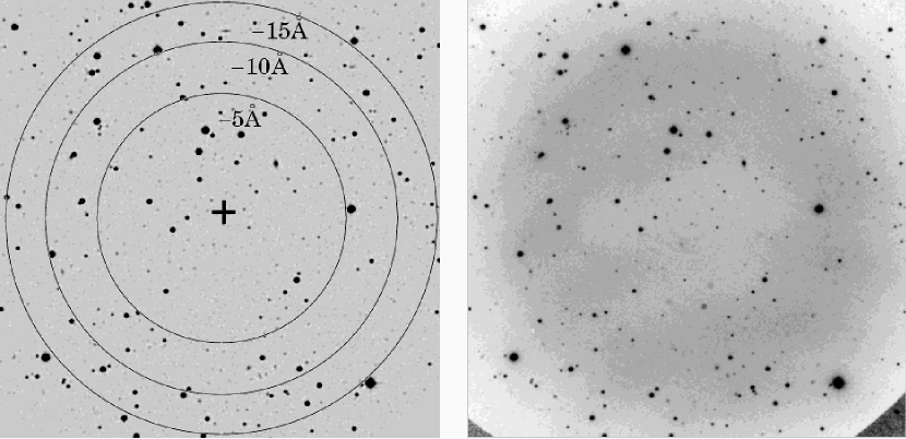
Figure 2.— Left: Illustration of the wavelength variation across an example TTF field. The image is the central $7^{\prime}\times 7^{\prime}$ about MRC B2021–208. Contours are drawn at 5Å intervals from the optical axis which is marked with a ’+’. Right: A night-sky ring before removal from the same image.

Flux calibrations were made by observing the spectrophotometric standards indicated in Table 1. For runs A, C, D and E, exactly the same scan parameters were employed as were used in the science observations. For scans B and F, the standards were observed in a subset (2 or 3) of the $Z$-values used in the science frames. In these latter cases the flux density was estimated assuming a linear relationship between the counts in the standard at different wavelengths.

3. Data reduction

All data reduction and ELG candidate selection algorithms detailed here were accomplished using IDL including custom scripts from the IDL astronomy users library as well as programs written by the authors.

3.1. Image production

Data reduction initially proceeded as it would for standard broad-band imaging. First the bias was removed from each image by subtracting the median of a bias frame or the median value of the overscan region. The data were flat-fielded at each $Z$ value using twilight-sky flats for scans A, B, E and F and dome flats for scans C and D.

Night-sky rings, caused by radial sensitivity to OH Meinel bands (see Figure 2), were removed by subtracting median values of the sky in concentric circles about the optical axis. These rings are actually ellipses, but for the etalon tilts and positions of the optical centres in this study are well approximated by circles. The night-sky rings were removed to within $4\%$ of the background level in the most affected images.

Images at a common $Z$ value were aligned by comparing positions of bright stars and co-added. Cosmic rays, bad pixels and ghosts were rejected. The positions of the cosmic rays in $x,y,Z$ space were recorded in order to cross-correlate their occurrence with that of ELGs at a later stage.

3.2. Catalogue creation

Object detection and aperture photometry was carried out using SExtractor (Bertin & Arnouts). Objects were detected in two ways:

1. SExtractor was used to identify objects at each $Z$ value in the scan separately and these were correlated by position after extraction.

2. The images from each scan were summed together and SExtractor was used to detect objects in this deep composite.

In both cases objects were identified as having 5 contiguous pixels at $3\sigma$ above noise in a median-smoothed image convolved with the scan’s worst seeing. Each method has its advantages in terms of locating ELGs. In the first case objects which are present at some $Z$ values but not others will not be diminished by the addition of extra noise. In the second instance, fainter continuum objects will be picked up, and the completeness limit of the catalogue will be deeper. These two methods were used purely to identify the positions at which to obtain aperture photometry in each image.

Photometry was then carried out using $3^{\prime\prime}$ diameter apertures. The objects were calibrated to a flux scale (erg s^-1 cm^-2) and AB magnitudes using the spectrophotometric standards indicated in Table 1. A small offset of typically 0.1 mag was applied to each object to correct for flux from the object falling outside the fixed aperture. This was calculated by comparing the magnitudes of a subset of $\sim 100$ objects measured within the $3^{\prime\prime}$ apertures with the magnitudes measured in larger ($5^{\prime\prime}-7^{\prime\prime}$) apertures. Corrections for galactic extinction (typically $A_{V}\sim 0.1$ mag) were made to each field using values from the NASA/IPAC Extragalactic Database.

The two catalogues, compiled from objects in individual bands and those identified from the combined scan, were analysed separately for the presence of candidate emission-line galaxies.

4. Identification of ELGs in TTF stacks

Objects detected by SExtractor at only one, two or three adjacent etalon values in the individual catalogues were identified first and set aside as ELG candidates. This initial sweep separated those objects for which only line emission was detectable. The search then proceeded to objects with line emission superposed on a continuum.

For objects detected individually in four or more images, a straight line was fitted to their fluxes in each band. The rms scatter, $\sigma$, about the line and the mean flux error, $\langle\Delta F\rangle$, were evaluated and the larger taken as the dominant source of error, $\sigma_{\mathrm{dom}}$. The background was then fitted iteratively as a straight line, rejecting the points that fell more than $\sigma_{\mathrm{dom}}$ above the line. A minimum of three points were retained to fit the background. Objects with peaks $>3\sigma$ above the fitted background were set aside as candidate line emitters. Those $Z$ values in which the flux was $>3\sigma$ above the background were identified as ‘line’ bands under two conditions:

1. Where there are two or more bands above the threshold, they should be adjacent.

2. If only one band is above the threshold, the (one or) two images adjacent to it are classified as ‘line’ bands. This is because line emission superposed on a detectable continuum is never narrow enough to be contained only in one $\sim 10$Å wavelength slice.

Candidate ELGs were also identified by considering the difference between the line and continuum magnitudes. ELG candidates are identified as objects with brightest magnitudes separated by more than three times the error from the average continuum magnitude. The selection is illustrated in Figure 3 for each field. A limit of $I(AB)>21$ is imposed on putative line emitters to avoid contamination of the sample at the bright end, where differences in luminosity between bands caused by light falling outside the small aperture become significant. At the redshifts probed by our sample we do not expect ELGs with $I(AB)>21$. This method was used successfully to find ELGs in the field of MRC B0450–221 in Paper 1 and in Hall et al. (2001).

Figure 3.— Difference between estimated peak and continuum magnitude (measured in all seven frames) plotted as a function of continuum magnitude for objects in the field of all quasars. The solid lines show the ELG selection criteria, ie: $I$(AB) $>21$ and continuum $-$ peak mag $=3\times$ the error in the average continuum magnitude. Objects qualifying as ELG candidates are marked as crosses. The quasar is marked by a circle.

All ELG candidates were cross-checked in $x,y,Z$ space with those of cosmic rays, and matches were excluded from the catalogue. Generally, the same objects were extracted by each selection method. However, the overlap was not complete – an indication that some candidates are missed by each process (see §4.1). As a final check, all candidates were examined by eye to ensure that no unusual cosmic rays or low-level ghosts were categorised as ELGs. A selection of candidates are shown in Figure 4.

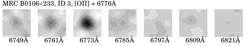
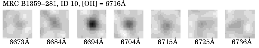
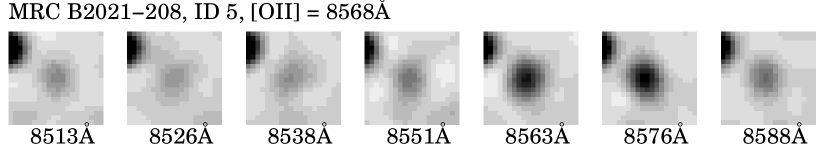
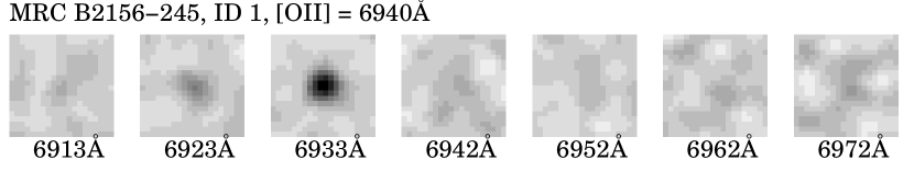
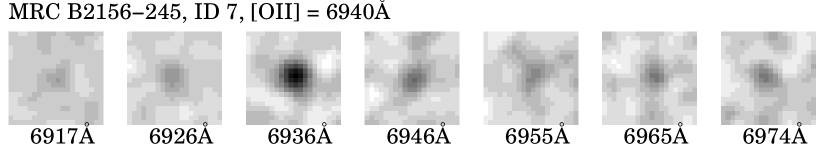
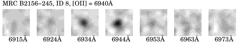
Figure 4.— Images showing some candidate line emitters in the fields of quasars. Each row corresponds to an object (with quasar name, ELG candidate ID and wavelength of redshifted [O ii] labelled top-left) at different wavelengths. Each frame is $7^{\prime\prime}\!\!.5$ square and is labelled with its central wavelength. North is up, East is left.

A total of 47 objects were identified as ELG candidates in our TTF observations. At least five candidates were discovered in each field. The characteristics of the ELG candidates found using TTF are shown in Table 2. Broad-band $I$ magnitudes are listed for those objects that have been detected as part of a separate program to detect clustering in the fields of RLQs Barr (2003); Barr et al. (2003). Redshifts are assigned based on the wavelength bin in which the emission peaks. The errors are assigned, conservatively, as the entire width of the wavelength bin. For those quasars for which [O ii] emission was detected, MRC B0413–210, MRC B1359–281 and MRC B2156–245, the redshift was checked for consistency with the published spectrum. In the latter two cases the peak in the [O ii] emission agrees with the spectra published in Baker et al. (1999). No occurrence of [O ii] is documented for MRC B0413–210 in Baker et al. For this quasar the wavelength calibration is not secure and is rederived assuming that [O ii] peaks at the quasar redshift (see §4.3.2). The [O ii] fluxes for MRC B1359–281 and MRC B2156–245 in Baker et al. (1999) were also found to be consistent, within the errors, with the present work.

Table 2Positions, redshift and luminosity characteristics of ELG candidates

MRC	ID	Position		$\lambda_{p}$	$z$([O ii])		Continuum		$F_{l}$		$W_{\lambda}$	$L$([O ii])
quasar		(J2000.0)					magnitude		($\times 10^{-16}$ erg			($\times 10^{41}$
		R.A.	Decl.	(Å)			$I(AB)$	$I$	s-1 cm-2)		(Å)	erg s-1)
(1)	(2)			(3)	(4)		(5)	(6)	(7)		(8)	(9)
B0106–233
	$1$	$01$ $09$ $\>\;3.08$	$-23$ $05$ $19.81$	$6754$	$0.812$ $\pm$	$0.003$	$>23.5$	$>21.0$	$0.3$$\pm$	$0.0$	$>24.2$	$0.8$$\pm$	$0.1$
	$2$	$01$ $09$ $\>\;4.10$	$-23$ $07$ $16.26$	$6773$	$0.817$ $\pm$	$0.003$	$>23.5$	21.8	$0.4$$\pm$	$0.0$	$>15.8$	$1.2$$\pm$	$0.1$
	$3$	$01$ $09$ $\>\;5.00$	$-23$ $07$ $27.67$	$6773$	$0.817$ $\pm$	$0.003$	$>23.5$	22.7	$1.3$$\pm$	$0.1$	$>93.5$	$3.8$$\pm$	$0.3$
	$4$	$01$ $09$ $\>\;0.95$	$-23$ $05$ $34.20$	$6767$	$0.816$ $\pm$	$0.003$	$>23.5$	22.4	$0.6$$\pm$	$0.1$	$>56.7$	$1.9$$\pm$	$0.3$
	$5$	$01$ $08$ $46.25$	$-23$ $06$ $23.55$	$6782$	$0.820$ $\pm$	$0.003$	$>23.5$	22.4	$0.2$$\pm$	$0.1$	$>11.6$	$0.6$$\pm$	$0.2$
B0413–210
	$1$	$04$ $16$ $\>\;8.85$	$-20$ $58$ $\>\;9.33$	$6730$	$0.806$ $\pm$	$0.002$	$>23.0$	$\cdots$	$0.5$$\pm$	$0.2$	$>28.0$	$1.5$$\pm$	$0.5$
	$2$	$04$ $15$ $54.14$	$-20$ $58$ $\>\;2.83$	$6731$	$0.806$ $\pm$	$0.002$	$>23.0$	$\cdots$	$0.4$$\pm$	$0.2$	$>22.4$	$1.2$$\pm$	$0.5$
	$3$	$04$ $16$ $\>\;5.16$	$-20$ $56$ $43.85$	$6738$	$0.808$ $\pm$	$0.002$	$>23.0$	$\cdots$	$1.0$$\pm$	$0.2$	$>50.4$	$2.9$$\pm$	$0.5$
	$4$	$04$ $16$ $\>\;7.03$	$-20$ $57$ $41.73$	$6730$	$0.806$ $\pm$	$0.002$	$>23.0$	$\cdots$	$0.2$$\pm$	$0.2$	$>9.8$	$0.6$$\pm$	$0.5$
	$5$	$04$ $15$ $58.06$	$-20$ $52$ $33.64$	$6719$	$0.803$ $\pm$	$0.002$	$>23.0$	$\cdots$	$0.6$$\pm$	$0.2$	$>29.4$	$1.8$$\pm$	$0.5$
	$6$	$04$ $16$ $\>\;4.08$	$-20$ $56$ $15.48$	$6737$	$0.808$ $\pm$	$0.002$	$>23.0$	$\cdots$	$0.6$$\pm$	$0.2$	$>30.8$	$1.8$$\pm$	$0.5$
	$7$	$04$ $15$ $56.70$	$-20$ $54$ $11.00$	$6738$	$0.808$ $\pm$	$0.002$	$>23.0$	$\cdots$	$0.4$$\pm$	$0.2$	$>18.2$	$1.1$$\pm$	$0.5$
	$8$	$04$ $15$ $52.58$	$-20$ $58$ $42.42$	$6731$	$0.806$ $\pm$	$0.002$	$>23.0$	$\cdots$	$0.9$$\pm$	$0.2$	$>56.0$	$2.6$$\pm$	$0.5$
	$9$	$04$ $16$ $14.41$	$-20$ $57$ $48.46$	$6717$	$0.802$ $\pm$	$0.002$	$>23.0$	$\cdots$	$1.5$$\pm$	$0.2$	$>182.0$	$4.5$$\pm$	$0.5$
	$10$	$04$ $16$ $\>\;2.51$	$-21$ $00$ $23.73$	$6741$	$0.809$ $\pm$	$0.002$	$>23.0$	$\cdots$	$0.3$$\pm$	$0.1$	$>11.2$	$0.9$$\pm$	$0.4$
	$11$	$04$ $16$ $17.77$	$-20$ $56$ $54.49$	$6740$	$0.808$ $\pm$	$0.002$	22.2	$\cdots$	$1.0$$\pm$	$0.2$	28.0	$2.8$$\pm$	$0.7$
B1359–281
	$1$	$14$ $01$ $54.79$	$-28$ $21$ $17.70$	$6699$	$0.797$ $\pm$	$0.002$	$>23.0$	21.5	$0.8$$\pm$	$0.1$	$>128.5$	$2.2$$\pm$	$0.4$
	$2$	$14$ $02$ $\>\;4.48$	$-28$ $23$ $\>\;6.59$	$6717$	$0.802$ $\pm$	$0.002$	$>23.0$	21.6	$1.1$$\pm$	$0.1$	$>186.7$	$3.2$$\pm$	$0.4$
	$3$	$14$ $01$ $51.94$	$-28$ $25$ $\>\;2.49$	$6702$	$0.798$ $\pm$	$0.002$	$>23.0$	$\cdots$	$0.8$$\pm$	$0.1$	$>130.6$	$2.2$$\pm$	$0.4$
	$4$	$14$ $02$ $22.02$	$-28$ $21$ $30.83$	$6711$	$0.801$ $\pm$	$0.002$	$>23.0$	$\cdots$	$1.1$$\pm$	$0.1$	$>187.7$	$3.2$$\pm$	$0.4$
	$5$	$14$ $02$ $13.67$	$-28$ $20$ $23.29$	$6707$	$0.800$ $\pm$	$0.002$	$>23.0$	22.5	$1.0$$\pm$	$0.1$	$>159.1$	$2.7$$\pm$	$0.4$
	$6$	$14$ $01$ $46.25$	$-28$ $22$ $28.22$	$6719$	$0.803$ $\pm$	$0.002$	$>23.0$	$\cdots$	$0.7$$\pm$	$0.1$	$>121.4$	$2.0$$\pm$	$0.4$
	$7$	$14$ $02$ $10.07$	$-28$ $18$ $\>\;7.38$	$6713$	$0.801$ $\pm$	$0.002$	21.2	$\cdots$	$1.2$$\pm$	$0.2$	10.2	$3.4$$\pm$	$0.5$
	$8$	$14$ $02$ $\>\;9.51$	$-28$ $18$ $\>\;1.09$	$6702$	$0.798$ $\pm$	$0.002$	22.4	$\cdots$	$0.6$$\pm$	$0.1$	21.4	$1.8$$\pm$	$0.4$
	$9$	$14$ $01$ $55.77$	$-28$ $18$ $41.35$	$6704$	$0.799$ $\pm$	$0.002$	22.0	$\cdots$	$1.3$$\pm$	$0.1$	101.0	$3.7$$\pm$	$0.4$
	$10$	$14$ $01$ $53.33$	$-28$ $20$ $34.70$	$6694$	$0.796$ $\pm$	$0.002$	22.1	21.9	$1.7$$\pm$	$0.1$	56.1	$4.8$$\pm$	$0.4$
B2021–208
	$1$	$20$ $24$ $38.52$	$-20$ $42$ $32.19$	$8525$	$1.287$ $\pm$	$0.003$	$>22.0$	$\cdots$	$0.7$$\pm$	$0.1$	$>51.0$	$6.6$$\pm$	$1.1$
	$2$	$20$ $24$ $44.03$	$-20$ $46$ $10.44$	$8544$	$1.292$ $\pm$	$0.003$	$>22.0$	$\cdots$	$1.1$$\pm$	$0.1$	$>85.5$	$10.0$$\pm$	$1.1$
	$3$	$20$ $24$ $39.45$	$-20$ $44$ $31.53$	$8528$	$1.288$ $\pm$	$0.003$	21.3	$\cdots$	$0.6$$\pm$	$0.1$	12.0	$5.6$$\pm$	$1.1$
	$4$	$20$ $24$ $41.10$	$-20$ $40$ $19.61$	$8556$	$1.296$ $\pm$	$0.003$	21.6	$\cdots$	$0.2$$\pm$	$0.2$	4.5	$2.0$$\pm$	$1.6$
	$5$	$20$ $24$ $41.63$	$-20$ $41$ $\>\;5.41$	$8576$	$1.301$ $\pm$	$0.003$	20.8	$\cdots$	$2.9$$\pm$	$0.2$	40.5	$27.7$$\pm$	$1.4$
	$6$	$20$ $24$ $46.52$	$-20$ $41$ $\>\;7.71$	$8520$	$1.286$ $\pm$	$0.003$	20.6	$\cdots$	$1.3$$\pm$	$0.1$	36.0	$12.0$$\pm$	$1.1$
	$7$	$20$ $24$ $52.36$	$-20$ $41$ $44.82$	$8525$	$1.287$ $\pm$	$0.003$	21.2	$\cdots$	$1.0$$\pm$	$0.1$	28.5	$9.3$$\pm$	$1.3$
B2037–234
	$1$	$20$ $40$ $\>\;8.42$	$-23$ $17$ $37.70$	$8053$	$1.161$ $\pm$	$0.004$	$>23.0$	22.0	$1.0$$\pm$	$0.2$	$>55.0$	$7.1$$\pm$	$1.4$
	$2$	$20$ $40$ $13.85$	$-23$ $16$ $40.02$	$8047$	$1.159$ $\pm$	$0.004$	$>23.0$	$>22.0$	$0.4$$\pm$	$0.2$	$>24.6$	$3.1$$\pm$	$1.3$
	$3$	$20$ $39$ $55.87$	$-23$ $14$ $38.31$	$8036$	$1.156$ $\pm$	$0.004$	$>23.0$	22.8	$1.0$$\pm$	$0.2$	$>41.6$	$6.8$$\pm$	$1.5$
	$4$	$20$ $39$ $57.91$	$-23$ $18$ $\>\;3.52$	$8072$	$1.166$ $\pm$	$0.004$	$>23.0$	21.9	$1.1$$\pm$	$0.2$	$>37.0$	$7.5$$\pm$	$1.1$
	$5$	$20$ $40$ $\>\;2.37$	$-23$ $15$ $\>\;6.76$	$8056$	$1.162$ $\pm$	$0.004$	21.8	21.5	$0.5$$\pm$	$0.2$	23.1	$3.4$$\pm$	$1.1$
B2156–245
	$1$	$21$ $59$ $27.74$	$-24$ $19$ $\>\;5.61$	$6933$	$0.860$ $\pm$	$0.002$	$>22.5$	21.6	$4.0$$\pm$	$0.3$	$>129.9$	$13.7$$\pm$	$0.9$
	$2$	$21$ $59$ $21.06$	$-24$ $14$ $11.40$	$6898$	$0.851$ $\pm$	$0.003$	$>22.5$	21.3	$1.4$$\pm$	$0.3$	$>36.0$	$4.6$$\pm$	$1.0$
	$3$	$21$ $59$ $36.87$	$-24$ $20$ $14.96$	$6955$	$0.866$ $\pm$	$0.002$	$>22.5$	21.3	$1.1$$\pm$	$0.2$	$>44.1$	$3.7$$\pm$	$0.7$
	$4$	$21$ $59$ $17.67$	$-24$ $20$ $10.58$	$6965$	$0.869$ $\pm$	$0.002$	$>22.5$	21.4	$0.4$$\pm$	$0.2$	$>17.4$	$1.3$$\pm$	$0.5$
	$5$	$21$ $59$ $42.20$	$-24$ $20$ $\>\;5.31$	$6946$	$0.864$ $\pm$	$0.002$	$>22.5$	21.3	$1.4$$\pm$	$0.2$	$>49.9$	$4.9$$\pm$	$0.8$
	$6$	$21$ $59$ $16.05$	$-24$ $17$ $\>\;5.88$	$6944$	$0.863$ $\pm$	$0.002$	21.3	21.1	$0.9$$\pm$	$0.2$	24.4	$3.0$$\pm$	$0.7$
	$7$	$21$ $59$ $18.30$	$-24$ $19$ $37.35$	$6936$	$0.861$ $\pm$	$0.002$	21.0	21.1	$3.6$$\pm$	$0.3$	85.8	$12.3$$\pm$	$1.0$
	$8$	$21$ $59$ $21.12$	$-24$ $18$ $48.38$	$6944$	$0.863$ $\pm$	$0.002$	20.4	21.3	$3.3$$\pm$	$0.2$	65.0	$11.1$$\pm$	$0.8$
	$9$	$21$ $59$ $25.45$	$-24$ $17$ $45.32$	$6948$	$0.864$ $\pm$	$0.002$	20.9	20.7	$2.4$$\pm$	$0.3$	53.4	$8.1$$\pm$	$0.9$

Note. — (1) quasar name; (2) ELG candidate ID; (3) peak wavelength; (4) redshift estimate (assuming emission is [O ii]); (5) TTF continuum magnitude, $I(AB)$ - these are denoted as limits equal to the limiting magnitude where there is no continuum magnitude; (6) $I$-band magnitudes from Barr et al. 2003 or Barr 2003 – these are left blank where no data are available and denoted as limits where there is coverage but no detection; (7) line flux; (8) observed equivalent width; (9) line luminosity (assuming emission is [O ii])

4.1. Completeness

There are two mechanisms which affect the completeness of the ELG candidate catalogues. The first is that objects with peak intensities below the magnitude completeness limit remain undetected. This is what is understood by completeness of catalogues in traditional broad-band imaging. There is an additional phenomenon in the present work, associated with the ELG line-fitting selection algorithm. If the line is not sufficiently distinguished from the continuum, as can happen if the line is faint, or the continuum bright, the candidate may not be detected. In this section we estimate the number of candidates missed by these two processes separately.

The cumulative number of all objects detected per half magnitude at each of the seven etalon values in each field are shown in Figure 5. These show that, with the exception of MRC B0106–233 which has substantially lower throughput in its reddest bands (see Figure 7 and §4.3.1), the completeness in a particular field are the same for all etalon values.

Figure 5.— Number of objects extracted at each etalon value in each field brighter than a given $I(AB)$ magnitude.

By extrapolating from the panels in Figure 5 and assuming a constant ratio between ELG candidates and other objects, per luminosity bin, we can estimate how many line emitters remain undetected because they fall below the completeness limit of the data. This analysis indicates that 7 candidates are missed in the field of MRC B0413–210 and 3 in the field of MRC B2037–234. The catalogues in all other fields are complete in that none of the candidates appear below the completeness limit of the data.

In order to test the algorithms which select objects based on fluxes above a fitted threshold, artificial catalogues were created. For each field $10000$ objects were simulated over a range of fluxes. These line emitters were created by deconvolving a Lorentzian curve with arbitrary peak wavelength and FWHM equal to the effective bandpass into seven bins. The resulting spectra were combined with the observational setup of each scan. The sky noise, efficiency and wavelength sensitivity were folded in to give catalogues of ELG candidates to submit to the selection algorithms.

The results are shown in Table 3 indicating that the selection algorithm is fairly robust. One line emitter is detected below the $50\%$ completeness level (in the field of MRC B0413–210), which suggests that one object is missed due to failings in the selection algorithm in this field. A similar analysis for the other five fields shows that no other candidates remain undetected.

Table 3Selection-algorithm completeness and predicted rates of interloper detections for different line emitters in the fields of the RLQs.

MRC	Selection-algorithm completeness				Interloping line emission					$N_{ELG}$
quasar	$\;\,100\%$	$75\%$	$50\%$		[O ii]	H$\alpha$	[O iii]
	($\times 10^{-16}$ erg s-1 cm-2)				$\lambda 3727$	$\lambda 6563$	$\lambda 5007$	$\lambda 4959$
				$z$	0.818	0.032	0.353	0.366
B0106–233	1.2 (4)	0.3 (1)	0.2 (0)	$V$	411	3	177	186
				$N_{s}$	0.6	$<0.1$	$<1$	$<1$		5
				$z$	0.807	0.026	0.345	0.358
B0413–210	0.4 (2)	0.3 (1)	0.3 (1)	$V$	551	3	233	244
				$N_{s}$	0.9	$<0.1$	$<1$	$<1$		11
				$z$	0.802	0.023	0.341	0.354
B1359–281	0.1 (0)	0.1 (0)	0.1 (0)	$V$	655	3	274	287
				$N_{s}$	1.0	$<0.1$	$<1$	$<1$		10
				$z$	1.299	0.306	0.711	0.728
B2021–208	0.3 (1)	0.2 (0)	0.2 (0)	$V$	709	206	522	532
				$N_{s}$	0.5	0.7	$<2$	$<2$		7
				$z$	1.15	0.22	0.60	0.62
B2037–234	0.5 (1)	0.4(0)	0.3 (0)	$V$	759	141	500	515
				$N_{s}$	0.5	0.4	$<2$	$<2$		5
				$z$	0.862	0.057	0.386	0.399
B2156–245	0.5 (1)	0.4 (0)	0.3 (0)	$V$	637	13	298	310
				$N_{s}$	1.0	$<0.1$	$<2$	$<2$		9

Note. — Selection-algorithm completeness indicates the efficiency of the ELG selection. The columns describe fluxes, in units of $10^{-16}$ erg s^-1 cm^-2, where the catalogues of artificial objects are $100\%$, $75\%$ and $50\%$ complete. Numbers of ELG candidates detected by TTF below this limit are indicated in parentheses. $z$: Redshift of line; $V$: Total volume surveyed at this redshift ($h^{3}_{70}$ Mpc³); $N_{s}$: Expected number of interlopers; $N_{ELG}$: Number of ELG candidates found.

There are several reasons why the completeness is different for each field. The photometric conditions and seeing in each scan is different; the sky brightness varies according to the wavelength; the increasing prevalence of OH emission lines at longer wavelengths makes the sky noisier and ELG detection consequently becomes more difficult. It is estimated that 10 ELG candidates are missed because their flux is below the completeness limit of the catalogue. Simulations of the ELG detection algorithm indicate that a single candidate is missed by this selection. Caution must be exercised before we add candidates to our sample, or enhance our statistics. The estimate of the number of objects missed depends on the presumption that the luminosity function of line emission traces that of the underlying population (as sampled by Figure 5). Because of the uncertainty inherent in this estimate, and because the actual brightness distribution of ELG candidates is not clear, we take a conservative approach and make no corrections for incompleteness in the analysis that follows.

4.2. Possible contaminants

Within the wavelength range of the observations, line emission from lower-redshift, star-forming galaxies may be observed. The strongest lines observed in these galaxies are generally due to H$\alpha$ $\lambda 6563$, [O ii] $\lambda 3727$ and [O iii] $\lambda\lambda 4959,5007$ and an estimate of the number of these interlopers is required before we evaluate our statistics.

We use the censuses of Gallego et al. (1995; $z<0.1$) and Cowie et al. (1997; $z>0.1$) to provide estimates of the ‘field’ density of star-forming galaxies at a given epoch. The numbers per unit SFR are converted to numbers per unit line luminosity using the empirical relationships for H$\alpha$ (Kennicutt, 1992, 1998) and [O ii] (Gallagher, Hunter & Bushouse, 1989; Kennicutt, 1998). The projected number of [O iii] emitters is harder to estimate because [O iii] strength is only poorly correlated with SFR. However, assuming that [O iii] is similar in luminosity to [O ii] in star-forming galaxies, we derived estimated numbers. These should be thought of as upper limits as in most ELGs [O iii] is weak in comparison to [O ii]. Corresponding analyses can be undertaken for other emission lines (eg: H$\beta$, H$\delta$, etc). However, lines other than H$\alpha$, [O ii] and [O iii] are faint, so only the strongest star-formers will contribute. These are rare and the fraction of ELGs of this type found serendipitously is likely to be negligible. The numbers of interlopers predicted by this method for each field are shown in Table 3.

The numbers given in Table 3 for [O ii] and H$\alpha$ emitters will be uncertain by a factor of a few. This is because of the scatter in the empirical luminosity-SFR relationship and the large uncertainties (at least a factor of 2) in the data of Cowie et al. The number of interlopers shown in Table 3 is further overestimated because of the restricted magnitude range of the detections ($21<I(AB)\lesssim 23$).

At high redshifts, the deep survey of Rhoads et al. (2000) predicts $\sim 4000$ deg^-2 z^-1 Ly$\alpha$ emitters in blank field surveys. This amounts to $\sim 1$ per TTF field. However, this figure is based on the detection of a single galaxy at $z=4.52$ with line flux of $1.7\times 10^{-17}$ erg s^-1 cm^-2 – below the completeness limits of our fields. This flux level, combined with the uncertainties inherent in extrapolating from a single object, and the high cosmic variance of Ly$\alpha$ emitters, makes it very difficult to estimate the number of such objects we should see. We therefore make no correction for contaminant Ly$\alpha$ emitters.

As well as star-forming galaxies, our search may detect line emission from AGN. However, AGN have a much lower co-moving number density than emission-line galaxies (Grazian et al. 2000; Hicks et al. 2002). This means that their contamination rate will not significantly affect the predictions for interlopers made above.

These estimates assume that we can treat star-forming galaxies as a homogeneously distributed population, which, of course, is not the case. ELGs are often found as multiples (eg: Hutchings et al. 1993; Hicks et al. 2002; Venemans et al. 2002). However, accounting for this variance is very difficult as the clustering of star-formers over a range of redshift is not clearly mapped. The predicted rate of interloping H$\alpha$ for most fields is $<0.1$, the expected number of [O iii] emitters is an upper limit based on the assumption that [O iii] traces SFR in the same way as [O ii], and imposing a magnitude cut at $I(AB)>21$ will cull lower redshift line emitters. Therefore, we expect objects detected by our TTF observations primarily to be [O ii] emitters.

The wavelength regions probed in this paper do not contain any sharp features that might arise in Galactic stars, so stars will not be a significant contaminant. We note that the wavelength range targetted in Paper 1 was clipped as a precaution against possible contamination by M-stars.

4.3. Notes on individual fields

4.3.1 MRC B0106–233

No evidence is seen for [O ii] emission from the quasar, consistent with the published nuclear spectrum (Baker et al., 1999). The analysis of this field is inhibited by the response of the blocking filter which drops off substantially in the red. This is less of a problem than appears to be the case from Figure 1 because only the central parts of each image sample the reddest wavelengths. An examination of the number of objects detected by SExtractor indicates that noticeably fewer objects are found at the reddest three $Z$ values. These are removed from any further analysis.

Five ELG candidates are picked out from what is, in terms of total objects, a sparse field (Figure 6). Two of the best candidates in the field (IDs 2 and 3) are situated within $10^{\prime\prime}$ of the quasar. Their emission also coincides with the quasar redshift, both having $z=0.817\pm 0.002$. Note that Figure 6 and the corresponding figures for other fields are created by combining the seven narrow-band images. They can therefore be considered as images taken through a passband of 70 – 100Å covering the redshifted [O ii]. ELG candidates in these images appear brighter than the continuum magnitude documented in columns 5 and 6 of Table 2 because the figures include, and indeed isolate, the line emission.

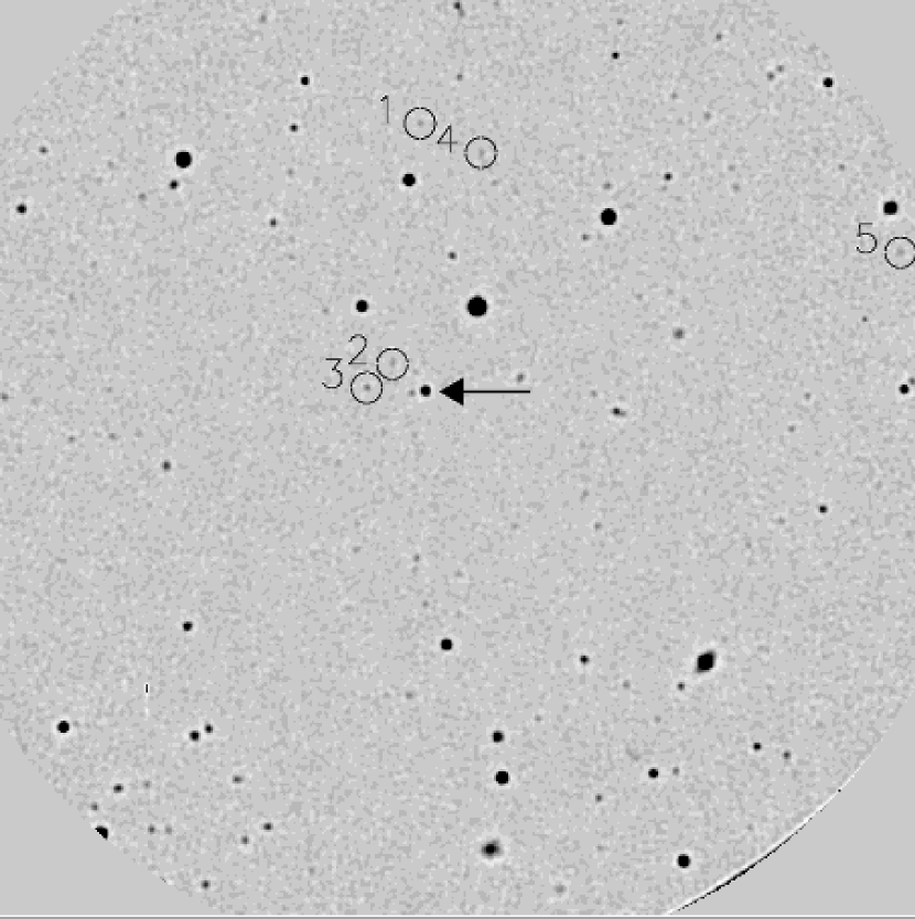
Figure 6.— The distribution of ELG candidates in the field of MRC B0106–233. The field of view is $7^{\prime}\!\!.4$ $\times$ $7^{\prime}\!\!.4$ of a composite of the seven (circular) TTF images. The quasar is marked with the horizontal arrow; North is up, East is left.

4.3.2 MRC B0413–210

The quasar brightens blueward of the position expected for [O ii] at $z=0.807$. However, the TTF wavelength calibration was taken nine hours before the data scan during which time the $Z,\lambda$ relation may have drifted. The redshift is originally determined from C iii], C iii] and Mg ii and does not catalogue the observed wavelength of [O ii] (Wilkes, 1986). For the purposes of this work it is assumed that the quasar is at $z=0.807$ and the peak flux in the TTF image of the RLQ is due to [O ii] emission. The wavelength solution was therefore adjusted 12Å redward to correct for the discrepancy. Note that this recalibration affects the wavelength space, not the amount of volume sampled or the flux calibration. The only analysis thus affected is the distribution of ELGs in velocity space. Figure 15 illustrates the effect that the adjustment has on the space density vs velocity histogram.

Assuming that the peak in the quasar brightness is due to [O ii], the flux response is that indicated in Figure 7. The morphology of the line emission is elongated slightly in the E – W direction, more-or-less aligned with the radio emission (Kapahi et al., 1998). However, the images in Figure 7 have mediocre spatial resolution (seeing $\approx$ $1^{\prime\prime}\!\!.0$). Nor is it out of the question that the ‘alignment’ is caused by a faint ELG located just East of the quasar. MRC B0413–210 is a small radio source (largest angular size $\sim 5^{\prime\prime}$) and the highest resolution radio map in Kapahi et al. (1998) is not detailed. Higher resolution radio and optical narrow-band imaging will be needed to ascertain the veracity of this alignment effect.

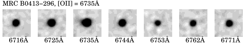
Figure 7.— TTF images of MRC B0413–210 in each band. The field of view in each panel is $11^{\prime\prime}\!\!.1$ $\times$ $11^{\prime\prime}\!\!.1$ and the central wavelength is indicated at each panel.

None of the eleven ELG candidates detected in this field is particularly strong, with only one object having an intrinsic equivalent width $>50$Å, and just one other with a detectable continuum magnitude (object 11). As with the field of MRC B0106–233 there is the coincidence of a pair of candidates with the quasar’s spatial position. There is also overlap in their redshifts, which are $z=0.805\pm 0.002$ and $z=0.808\pm 0.002$, well matched to the quasar redshift. There is no further obvious clustering of ELG candidates in the field of MRC B0413–210 (Figure 8).

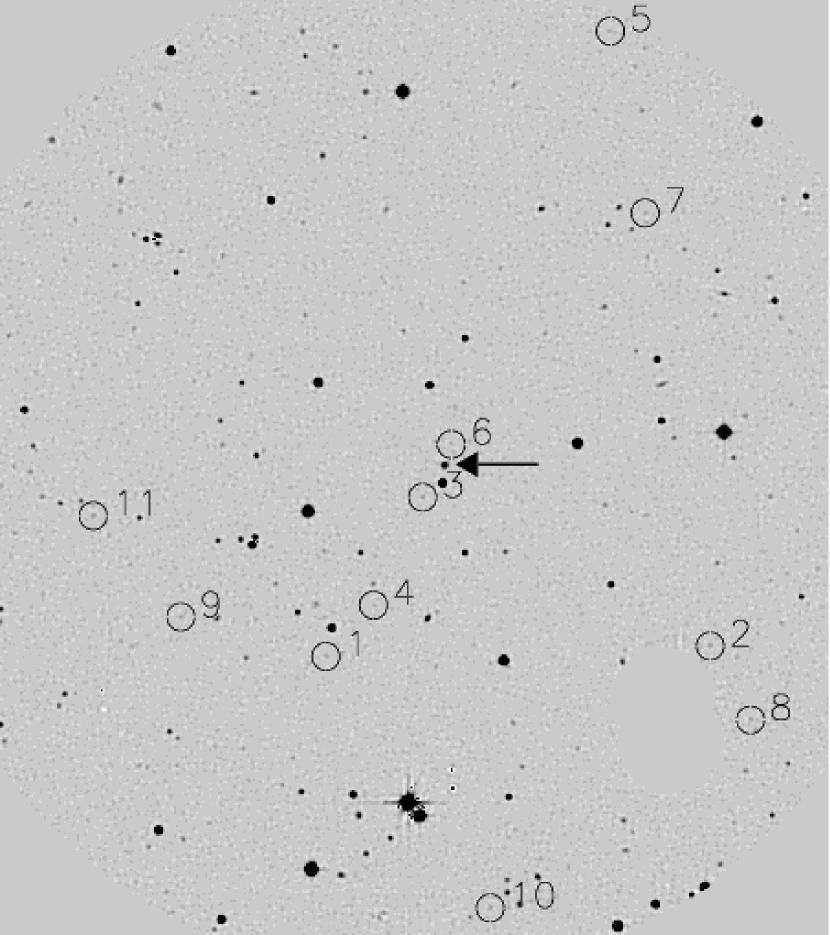
Figure 8.— The distribution of ELG candidates in the field of MRC B0413–210. The image is a composite of the seven TTF bands cut to $7^{\prime}\!\!.4$ $\times$ $8^{\prime}\!\!.3$ about the quasar (marked with the horizontal arrow). North is up, East is left.

4.3.3 MRC B1359–281

The quasar shows a strong peak in brightness at the wavelength of [O ii] at $z=0.802$, although its morphology remains optically unresolved. In radio terms, MRC B1359–281 is a compact steep-spectrum source (see Kapahi et al. 1998) .

Ten ELG candidates are detected, including seven objects with $W_{\lambda}>50$Å. Apart from a pair $\sim 5^{\prime}$ from the quasar, there is no clustering of these objects (Figure 9).

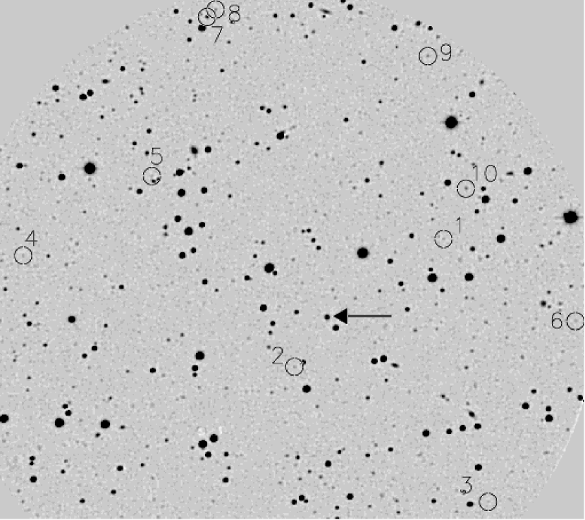
Figure 9.— The distribution of ELG candidates in the field of MRC B1359–281. The field of view is $8^{\prime}\!\!.3$ $\times$ $7^{\prime}\!\!.4$ of a composite of the seven TTF bands. The quasar is marked with the arrow. North is up, East is left.

The quasar was imaged as part of a broad-band program to detect clustering of passively-evolving ellipticals in the fields of RLQs (Barr et al. 2003). No evidence for a group or cluster of red galaxies was found.

4.3.4 MRC B2021–208

There is no significant peak in the quasar flux at 8568Å, the wavelength expected of [O ii] at $z=1.299$. Nor does the morphology change from that of an unresolved point source. No obvious [O ii] emission is seen in the published spectrum (Murdoch, Hunstead & White 1984).

Two objects with continuum magnitude brighter than the $I(AB)=21$ magnitude cutoff are found to display very strong line emission. A first-ranked cluster member at the redshift of the quasar would have $I\sim 21-22$ (Eales, 1985; Snellen et al., 1996). Emission-line galaxies at $z=1.299$ should be fainter than this, so it seems likely that ELG candidates 5 and 6 are not [O ii] emitters at $z=1.299$. The strongest expected line associated with ELGs is H$\alpha$ which the TTF setup in the present case is sensitive to at $z=0.30$. The number of H$\alpha$ interlopers within the volume of observation is predicted to be $\sim 1$. It is therefore likely that the line emitters with $I<21$ are H$\alpha$ sources at $z=0.3$.

In terms of spatial position, the ELG candidates locate themselves primarily to the NE of the quasar (Figure 10). However, the spatial clustering is rather loose and three of these objects are the brightest in the field. If these are indeed not [O ii] emitters, they may be a group of H$\alpha$ emitters at $z=0.30$. Deep spectroscopy will be required to test this hypothesis.

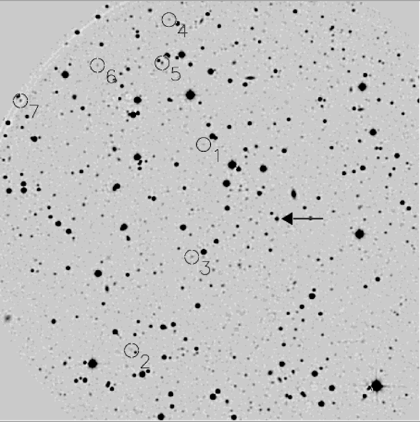
Figure 10.— The distribution of ELG candidates in the field of MRC B2021–208. The field of view is $7^{\prime}\!\!.4$ $\times$ $7^{\prime}\!\!.4$. The image is a composite of the seven TTF bands and the quasar is marked with a horizontal arrow. North is up, East is left.

4.3.5 MRC B2037–234

The quasar is faint, with magnitude $I(AB)\approx 21$. This makes it difficult to characterise any [O ii] emission, nuclear or extended. No strong [O ii] emission from MRC B2037–234 is seen. There is no published optical spectrum for this source and the redshift is more uncertain than the other quasars observed in this paper.

Only five ELG candidates are detected in this field. None is an especially strong line emitter, nor is any one found at the wavelength expected for [O ii] at $z=1.15$. As indicated in Table 3, there is no clear excess of ELG candidates in this field at the quasar redshift. The numbers are consistent with the expected number of interlopers and field galaxies. The candidates are spread across the field, with no sign of clustering (Figure 11).

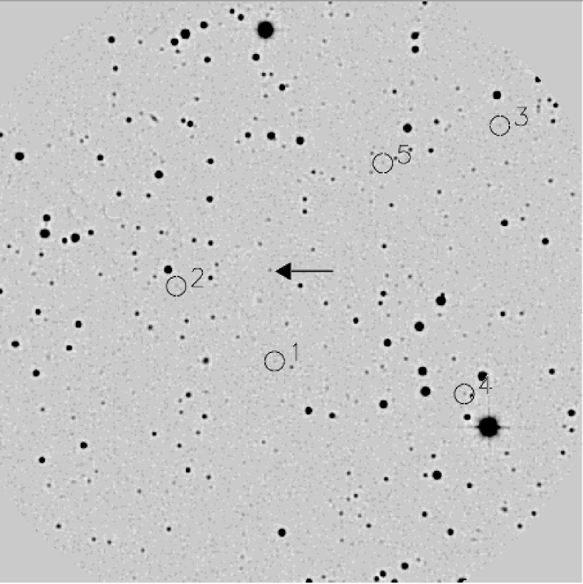
Figure 11.— The distribution of ELG candidates in the field of MRC B2037–234. The field of view is $7^{\prime}\!\!.4$ $\times$ $7^{\prime}\!\!.4$ of a composite of the seven TTF bands and the quasar is marked by an arrow. North is up, East is left.

4.3.6 MRC B2156–245

The quasar brightness peaks at 6949Å, $\sim 9$Å redward of the wavelength of [O ii] at $z=0.862$, which may indicate that the $Z,\lambda$ relation has drifted. Indeed, the wavelength calibration used in this field comes from the previous night. However, the published spectrum of MRC B2156–245 Baker et al. (1999) has [O ii] at 6952Å, consistent with the TTF result. No adjustment to the wavelength solution is made.

The [O ii] emission from MRC B2156–245 appears to align itself $\sim$ NW – SE (Figure 12). Recent MERLIN images show sub-arcsecond mini-lobes extending NW and E of the quasar nucleus (de Silva et al., in preparation).

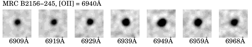
Figure 12.— TTF images of MRC B2156–245 in each band. The field of view in each panel is $11^{\prime\prime}\!\!.1$ $\times$ $11^{\prime\prime}\!\!.1$ and the central wavelength is indicated at each panel.

There are a number of strong line emitters found in this field. Seven out of nine have emission consistent with [O ii] at $z=0.862$. Moreover, they appear to congregate to the SW of the quasar. This is the site of a cluster of galaxies found in Barr (2003). Figure 13 shows that, while the ELG candidates appear near the red galaxy overdensity, they avoid the site of peak clustering. This supports the view that the edges, rather than cores of clusters of galaxies, are predominantly the sites of star formation activity.

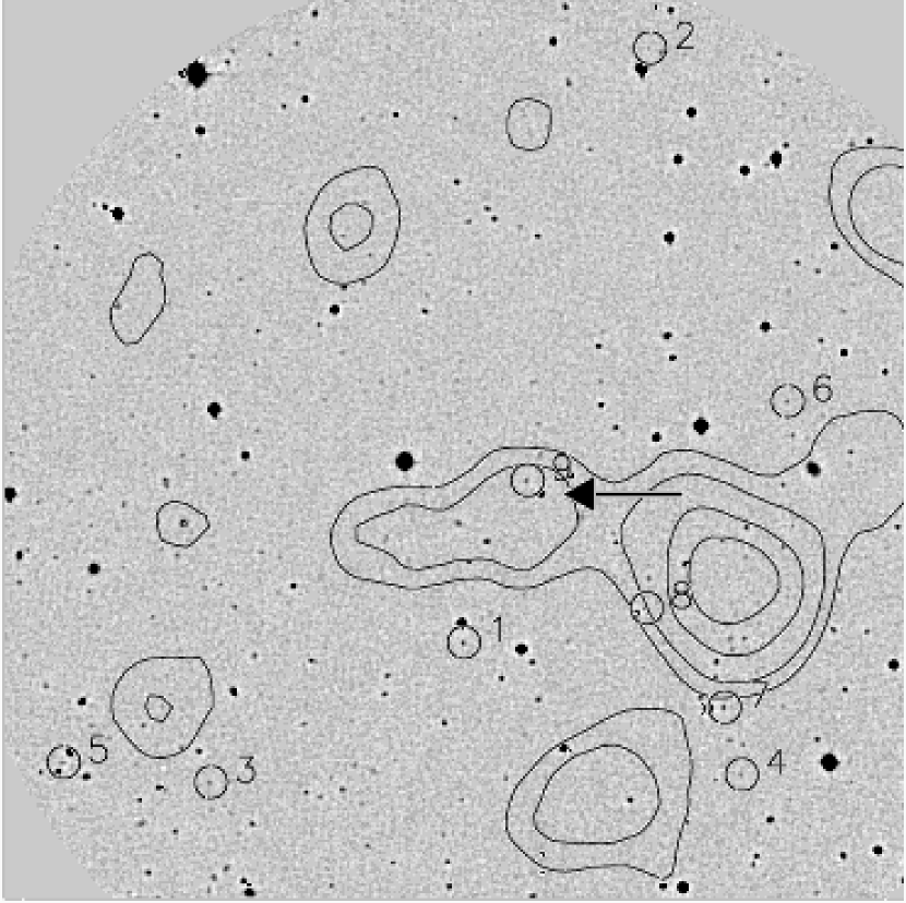
Figure 13.— The distribution of ELG candidates in the field of MRC B2156–245. The field of view is $7^{\prime}\!\!.4$ $\times$ $7^{\prime}\!\!.4$ and the quasar is marked with the horizontal arrow. The image is a part of composite of the seven TTF bands. North is up, East is left. Contours represent the surface density of galaxies with colours of passively-evolving elliptical galaxies at $z=0.862$ from Barr (2003). The levels are 2, 3, 5 and 7 $\times$ the Poissonian noise of similarly-coloured galaxies.

5. Discussion

In this paper we have examined the fields of six quasars and find forty-seven new ELG candidates. The number of candidates about each quasar varies from the number expected from field surveys (eg: MRC B2037–324) to overdensities of $\sim 10$ times (MRC B0413–210, MRC B1359–281). Previous studies have shown that MRC B2156–245 resides on the edge of a rich cluster of galaxies (Barr, 2003). The other five quasars have either not been examined for evidence of galaxy clustering (due to observing constraints) or have environmental richnesses consistent with the field (Barr, 2003; Barr et al., 2003).

We now consider the ELG properties and environments of all seven MQS quasars targetted with TTF, including the 17 ELG candidates (3 spectroscopically confirmed) detected in the field of MRC B0450–221 at $z=0.9$ described in Paper 1. Clear evidence for a rich cluster of galaxies in the MRC B0450–221 field was presented in Paper 1.

We note that followup spectroscopy is necessary to determine the nature of the ELG candidates. For the forthcoming discussion we assume the line is indeed [O ii] for all candidates except the two brightest objects in the field of MRC B2021–208 (see §4.3.4). In Paper 1, spectroscopic follow-up found one low-redshift interloper out of seven targets, which agrees with the number expected from the analysis described in Section 4.2. Therefore, as the determination of interlopers in this paper is essentially the same as that in Paper 1, no great diminution of the statistics presented here is expected.

5.1. Extended [O ii] emission around quasar host galaxies

It is well known that radio-loud AGN at moderate to high redshifts exhibit strong alignments between their optical-line and radio emission (eg: McCarthy 1993; Rush et al. 1997; Axon et al. 2000; Hutchings, Morris & Crampton 2001). Indeed, extended [O ii] emission is common around 3C quasars at comparable redshifts to the quasars in our sample (eg: Bremer et al. 1992). We note that evidence of such a phenomenon in this work exists for two sources (MRC B0413–210 and MRC B2156–245). However, the resolution of each image precludes detailed optical mapping of these regions.

5.2. The distribution of ELG candidates about quasars

Figure 14 plots the surface density of candidate [O ii] emitters against projected distance from the quasar. There is a peak in the surface density of ELG candidates within $250$ kpc of the quasars, and also a smaller overdensity at $500-1000$ kpc from the quasar. The first signature appears to arise from ELG close companions to the quasars, e.g. a pair of ELGs lying within $10^{\prime\prime}$ of MRC B0106–233, and similarly for MRC B0413–210. The latter excess occurs at distances consistent with the scale lengths of galaxy clusters about AGN at these redshifts Hall & Green (1998); Nakata et al. (2001); Bremer et al. (2002); Barr et al. (2003).

Figure 14.— The projected distances of ELG candidates about the quasars. The $1\sigma$ error bars based on the number of objects per bin are shown.

In the six new fields presented in this paper, no further examples of strongly clustered ELG groups similar to that seen in the field of MRC B0450–221 (Paper 1) are found, apart from the quasar companions. Weak clustering of ELG candidates is likely, but the small numbers preclude a detailed clustering analysis. For example, ELG candidates are seen solely NE of MRC B2021–208 or SW of MRC B2156–245.

Figure 15 shows the distribution in velocity space of [O ii] candidates detected with TTF about the quasars. The left panel indicates that the average space density of these objects from $-1000\lesssim v_{\mathrm{quasar}}\lesssim 500$ km s^-1 is $\approx 0.01$ Mpc^-3, ten times greater than the $\lesssim 0.001$ Mpc^-3 expected from field surveys (Cowie et al., 1997). The right panel in Figure 15 plots the number density vs velocity histogram for MRC B0450–221 and MRC B2156–245, two quasars known to reside in rich clusters of galaxies (Baker et al., 2001; Barr, 2003). These fields clearly show a large overdensity of ELG candidates about the quasar redshift. The spread in velocities seen ($\sigma\approx 750$ km s^-1, by fitting a simple Gaussian distribution) is comparable with the average velocity dispersion for Abell richness class 2 clusters of $\sim 800$ km s^-1 Yee & Ellingson (2003).

Figure 15.— Left: The space density of ELG candidates detected with TTF about quasars in this work as a function of velocity relative to the quasar redshift. The dashed line shows the distribution before recalibrating the wavelength solution from MRC B0413–210. The expected number of ELGs with these properties in the field is expected to be $\lesssim 0.001$ Mpc^-3 at these redshifts (Cowie et al. 1997). Right: The same but restricted to two quasars known to reside in or near clusters of galaxies (MRC B0450–221, MRC B2156–245). The solid line denotes the best fit Gaussian curve to the points ($\sigma$ is 750 km s^-1). Error bars are $1\sigma$ based on the number of objects per velocity bin; note the different ranges on the y-axes.

5.3. Equivalent widths and star formation rates

The observed equivalent widths for the ELG candidates in this paper lie in the range $\sim 10-200$Å, corresponding to $\sim 5-100$Å in the rest frames of the quasars. Figure 16 shows the distribution of the intrinsic $W_{\lambda}$. This distribution of equivalent widths is consistent with the field survey of Hogg et al. (1998) of [O ii] emission-line galaxies in the field with $0.8<z<1.3$.

Figure 16.— Histogram of rest frame equivalent widths, $W_{\lambda}$, for ELG candidates in this work. The unfilled parts of the histogram represent those objects without a continuum magnitude whose value of $W_{\lambda}$ is a lower limit.

Figure 17 shows the candidate ELG luminosity function, assuming that the emission is [O ii]. Also displayed is the luminosity function of local [O ii] emitters (Gallego et al., 2002) as well as two representations of high-redshift field surveys of star-forming galaxies (Cowie et al., 1997; Hogg et al., 1998) adjusted to our adopted cosmology. The number of [O ii] line emitters per unit luminosity in the vicinity of quasars at $0.8\lesssim z\lesssim 1.3$ is $\sim 100$ times greater than those found locally. At $L$([O ii]) $<10^{42}$ erg s^-1, the density of [O ii] emitters near RLQs is $2-5$ times greater than the field at similar redshifts. This suggests that at $z\gtrsim 0.8$, quasars are found in regions of above-average star formation activity. There is also a variation in the strength and number of ELG candidates found about quasars, eg: MRC B2037–234 has a number of line emitters consistent with no overdensity in contrast to the clear clustering of strong ELG candidates near MRC B2156–245.

Figure 17.— Cumulative density of objects brighter than a given threshold vs [O ii] luminosity. Squares represent data points for the quasars in this paper. Circles are $0.3<z<1.3$ ELGs from the [O ii] survey of Hogg et al. (1998). Stars represent points with $0.8<z<1.6$ from the Cowie et al. (1997) $B$-band survey converted to [O ii] luminosity using the conversion of Gallagher et al. (1989). Triangles represent the local [O ii] luminosity function of Gallego et al. (2002). All points have been adjusted to a $H_{0}=70$ km s^-1 Mpc^-1, $\Omega_{\Lambda}=0.7$ cosmology. Error bars are the root variance of the number of objects in each luminosity bin and are therefore not independent.

To estimate the SFR from [O ii] luminosity we use the empirical conversion of Gallagher et al. (1989):

$$\mathrm{SFR}\approx 1\>\hbox{M${}_{\odot}$}\>\mathrm{yr}^{-1}\left(\frac{L(\mathrm{[OII]})}{10^{41}\>\mathrm{erg}\>\mathrm{s}^{-1}}\right)$$

This conversion is uncertain by a factor of a few due to the scatter in the samples used to calibrate the relationship. However, most estimators of SFR are reasonably insecure because the estimates are highly model dependent and include assumptions about the IMF, metallicity and extinction (see the review by Kennicutt 1998).

The resulting distribution of star formation rates is shown in Figure 18. The SFRs span a range of $\sim 1-50$ M_⊙yr^-1 with a median value of $4$ M_⊙yr^-1, that is also consistent with those of field galaxies at similar redshifts (Cowie et al., 1997; Hogg et al., 1998; Hicks et al., 2002).

Figure 18.— Histogram of star formation rates for ELG candidates in this work inferred from [O ii] line luminosities using the relationship of Gallagher et al. (1989). The unfilled parts of the histogram represent those objects without a continuum magnitude whose SFR is a lower limit.

Caution must be exercised in interpreting the above results. Vagaries in the basic properties of ELGs at $z\sim 1$ such as gas ionization and extinction make it difficult to compare samples selected using different methods. The empirical conversion from $L$([O ii]) to SFR is uncertain, and there is variation in the number of ELG candidates found per field, as well as a small number found overall. For these reasons, any quantitative analysis of the luminosity function and star formation activity is likely to be equivocal.

5.4. Line emitters about AGN at other redshifts

Our data provide a comparison with the detections of line emitters of different types in the fields of AGN at other redshifts. Surveys of this type vary in depth and sensitivity but yield surprisingly consistent results. The [O ii] narrow-band survey of Hutchings et al. (1993) of the fields of seven quasars and radio galaxies at $z\sim 1.1$ found a density of $0.006-0.04$ Mpc^-3 ELG candidates, though the limiting SFR is not made explicit.

Teplitz, Malkan & McLean (1998) in their infrared search for H$\alpha$ emitters near $2.3<z<2.5$ quasars found $0.0135\pm^{0.0055}_{0.0035}$ Mpc^-3. The average inferred SFR of these candidates was 50 M_⊙yr^-1 and their density is $\sim 3$ times that of field surveys at a similar redshift. Hall et al. (2001) also detected an overdensity of candidate H$\alpha$ emitters about radio-loud quasars $\sim 3$ times over the field, this time at $z\sim 1.5$.

The studies of Pentericci et al. (2000), Kurk et al. (2001) and Venemans et al. (2002) have found tens of Ly$\alpha$ emitters around radio galaxies at $z=2.16$ and $z=4.10$. The space density of these emitters is $0.01$ Mpc^-3 in both cases and Kurk et al. claim to be sensitive to star formation rates $\gtrsim 1$ M_⊙yr^-1. However, it remains notoriously difficult to convert Ly$\alpha$ luminosity to SFR at $z>2$ because of the effect of intervening neutral hydrogen clouds.

These studies show that powerful radio sources are typically found in fields with overabundances of line emitters. Overdensities typically range from $2-15$ times those of field surveys and velocity dispersions are $\sim 300-1000$ km s^-1.

Our TTF study finds a space density of ELG candidates of $\sim 0.01$ Mpc^-3 with SFR $\gtrsim 1$ M_⊙yr^-1. The quasars detailed here inhabit quantitatively similar environments to those at similar and higher redshifts. Taken together these results suggest that powerful radio sources trace similarly-overdense regions of active star-formation over a great range in redshift.

6. Conclusions

• We demonstrate that it is possible to isolate star-forming galaxies at $0.8<z<1.3$ using tunable-filter observations. We have detected forty-seven new ELG candidates in the fields of six quasars. The candidates are selected on the basis of luminosity changes across narrow wavelength ranges centred on redshifted [O ii].

• Radio-loud quasars at $0.8<z<1.3$ are found in regions of above-average star formation activity. The number density of ELG candidates about the quasars in our sample is $\sim 100$ times that of local [O ii] emitters and $2-5$ times the number found in spectroscopic field surveys at $0.8\lesssim z\lesssim 1.5$ at $L$([O ii]) $<10^{42}$ erg s^-1.

• On average, the space density and velocity distributions of ELG candidates peak about the quasars. However, there is variance from field to field. The number of candidates found in individual quasar fields varies from that expected from field surveys, to overdensities of $\sim 10$ times.

• The equivalent widths and inferred star formation rates of ELG candidates in the quasar fields typically range between $5<W_{\lambda}<100$Å and $1<\mathrm{SFR}<50$ M_⊙yr^-1. The median SFR is $4$ M_⊙yr^-1. These values are consistent with those seen in the field at the same redshifts.

• The ELG candidate distributions, velocity dispersions and star formation rates at $z\sim 1$ detailed in this paper are consistent with studies of line emitters in the fields of AGN at $1<z<4$. Radio sources inhabit actively star-forming regions over a wide range in redshift.

References

- Axon et al. (2000) Axon, D. J., Capetti, A., Fanti, R., Morganti, R., Robinson, A., & Spencer, R. 2000, AJ, 120, 2284
- Balogh et al. (1997) Balogh, M. L., Morris, S. L., Yee, H. K. C., Carlberg, R.G., & Ellingson, E. 1997, ApJ, 488, L75
- Balogh et al. (1998) Balogh, M. L., Schade, D., Morris, S. L., Yee, H. K. C., Carlberg, R.G., & Ellingson E. 1998, ApJ, 504, L75
- Baker et al. (1999) Baker, J. C., Hunstead, R. W., Kapahi, V. K., & Subrahmanya, C. R. 1999, ApJS, 122, 29
- Baker et al. (2001) Baker, J. C., Hunstead, R. W., Bremer, M. N., Bland-Hawthorn, J., Athreya, R. M., & Barr, J. M. 2001, AJ, 121, 1821.
- Barr (2003) Barr, J. M. 2003, PhD Thesis, University of Bristol
- Barr et al. (2003) Barr, J. M., Bremer, M. N., Baker, J. C., & Lehnert, M. D. 2003, MNRAS, 346, 229
- Bertin & Arnouts (1996) Bertin, E., & Arnouts, S. 1996, AASS, 117, 393
- (9) Bland-Hawthorn, J., & Jones, D. H. 1998a, PASA, 15, 44
- (10) Bland-Hawthorn, J., & Jones, D. H. 1998b, Proc. SPIE, Optical Astronomical Instrumentation, Sandro D’Odorico; Ed., 3355, 855
- Boyle & Terlevich (1998) Boyle, B. J., Terlevich, R. J., 1998, MNRAS, 293, L49
- Bremer et al. (1992) Bremer, M. N., Crawford, C. S., Fabian, A. C., & Johnstone, R. M. 1992, MNRAS, 254, 614
- Bremer et al. (2002) Bremer, M. N., Baker, J. C., & Lehnert, M. D. 2002, MNRAS, 337, 470
- Butcher & Oemler (1984) Butcher, H., & Oemler, A. 1984, ApJ, 285, 426
- Cardiel et al. (2003) Cardiel, N., Elbaz, D., Schiavon, R. P., Willmer, C. N. A., Koo, D. C., Phillips, A. C., & Gallego, J. 2003, ApJ, 584, 76
- Cowie et al. (1997) Cowie, L. L., Hu, E. M., Songaila, A., & Egami E. 1997, ApJ, 481, L9
- Cowie, Songaila & Barger (1999) Cowie, L. L., Songaila, A., & Barger, A. J. 1999, AJ, 118, 603
- Dressler & Gunn (1992) Dressler, A., & Gunn, J. E. 1992, ApJS, 42, 565
- Eales (1985) Eales, S. A. 1985, MNRAS, 217, 149
- Ellingson, Yee & Green (1991) Ellingson, E., Yee, H. K. C., & Green, R. F. 1991, ApJ, 371, 49
- Ellis et al. (1996) Ellis, R. S., Colless, M., Broadhurst, T., Heyl, J., & Glazebrook K. 1996, MNRAS, 280, 235
- Finn, Impey, & Hooper (2001) Finn, R. A., Impey, C. D., & Hooper, E. J. 2001, ApJ, 557, 578
- Gallagher, Hunter & Bushouse (1989) Gallagher, J. S., Hunter, D. A., & Bushouse, H. 1989, AJ, 97, 700
- Gallego et al. (1995) Gallego, J., Zamorano, J., Aragón-Salamanca, A., & Rego, M. 1995, ApJ, 455, L1
- Gallego et al. (2002) Gallego, J., García-Dabó, C. E., Zamorano, J., Aragón-Salamanca, A., & Rego, M. 2002, ApJ, 570, L1
- Grazian et al. (2000) Grazian, A., Cristiani, S., D’Odorico, V., Omizzolo, A., & Pizzella, A. 2000, AJ, 119,2540
- Hall & Green (1998) Hall, P. B. & Green, R. F. 1998, ApJ, 507, 558
- Hall et al. (2001) Hall, P. B., et al. 2001, AJ, 121, 1840
- Hammer et al. (1997) Hammer, F., et al. 1997, ApJ, 481, 49
- Hicks et al. (2002) Hicks, E. K. S., Malkan, M. A., Teplitz, H. I., McCarthy, P. J., & Yan, L. 2002, ApJ, 581, 205
- Hogg et al. (1998) Hogg, D. W., Cohen, J. G., Blandford, R., & Pahre, M. A. 1998, ApJ, 504, 622
- Hutchings et al. (1993) Hutchings, J. B., Crampton, D., & Persram, D. 1993, AJ 106, 4
- Hutchings et al. (2001) Hutchings, J. B., Morris, S. L., & Crampton, D. 2001, AJ, 121, 80
- Jones & Bland-Hawthorn (2001) Jones, D. H., & Bland-Hawthorn, J. 2001, ApJ, 550, 593
- Jones et al. (2002) Jones, D. H., Shopbell, P. L., & Bland-Hawthorn, J. 2002, MNRAS, 329, 759
- Kapahi et al. (1998) Kapahi, V. K., Athreya, R. M., Subrahmanya, C. R., Baker, J. C., Hunstead, R. W., McCarthy, P. J., & van Breugel, W. 1998, ApJS, 118, 327
- Kennicutt (1992) Kennicutt, R. C. 1992, ApJ, 388, 310
- Kennicutt (1998) Kennicutt, R. C. 1998, ARA&A, 36, 189
- Khochfar & Burkert (2001) Khochfar, S., & Burkert, A. 2001, ApJ, 561, 517
- Kurk et al. (2001) Kurk, J. D., Pentericci, L., Röttgering, H. J. A., & Miley, G. K. 2001, Astrophysics and Space Science Supplement, 277, 543
- Lacey & Cole (1993) Lacey, C., & Cole, S. 1993, MNRAS, 262, 627
- Laing et al. (1983) Laing, R. A., Riley, J. M., & Longair, M. S. 1983, MNRAS, 204, 151
- Lilly et al. (1996) Lilly, S. J., Le Fevre, O., Hammer, F., & Crampton, D. 1996, ApJ, 460, L1
- Madau et al. (1996) Madau, P., Ferguson, H. C., Dickinson, M. E., Giavalisco, M., Steidel, C. C., & Fruchter, A. 1996, MNRAS, 283, 1388
- Madau, Pozzetti & Dickinson (1998) Madau, P., Pozzetti, L., & Dickinson, M. 1998, ApJ, 1998, 498
- McCarthy (1993) McCarthy, P. J. 1993, ARA&A, 31, 639
- McLure & Dunlop (2001) McLure, R. J., & Dunlop, J. S. 2001, MNRAS, 321, 515
- Miller & Owen (2003) Miller, N. A., & Owen, F. N. 2003, AJ, 125, 2427
- Murali et al. (2002) Murali, C., Katz, N., Hernquist, L., Weinberg, D. H., & Davé, R. 2002, ApJ, 571, 1
- Murdoch et al. (1984) Murdoch, H. S., Hunstead, R. W., & White, G. L. 1984, PASA, 5, 341
- Nakata et al. (2001) Nakata, F. et al. 2001, PASJ, 53, 1139
- Pentericci et al. (2000) Pentericci, L., et al. 2000, A&A, 361, L25
- Rhoads et al. (2000) Rhoads, J. E., Malhotra, S., Dey, A., Stern, D., Spinrad, H., & Jannuzi, B. T. 2000, ApJ,545, L85
- Rush et al. (1997) Rush, B., McCarthy, P. J., Athreya, R. M., & Persson, S. E. 1997, ApJ, 484, 163
- Snellen et al. (1996) Snellen, I. A. G., Bremer, M. N., Schilizzi, R. T., Miley, G. K., & van Ojik, R. 1996, MNRAS, 279, 1294
- Teplitz et al. (1998) Teplitz, H. I., Malkan, M., & McLean, I. S. 1998, ApJ, 506, 519
- Venemans et al. (2002) Venemans, B. P., et al. 2002, ApJ, 569, L11
- Wang et al. (2004) Wang, J. X., et al. 2004, ApJ, 608, L21
- Wilkes (1986) Wilkes, B. J. 1986, MNRAS, 218, 331
- Wold et al. (2000) Wold, M., Lacy, M., Lilje, P. B., & Serjeant, S. 2000, MNRAS 316, 267
- Wold et al. (2001) Wold, M., Lacy, M., Lilje, P. B., & Serjeant, S. 2001, MNRAS, 323, 231
- Yee & Green (1984) Yee, H. K. C., & Green, R. F. 1984, ApJ, 280, 79
- Yee & Ellingson (2003) Yee, H. K. C., & Ellingson, E. 2003, ApJ, 585, 215