Spectral Classification of Quasars in the Sloan Digital Sky Survey: Eigenspectra; Redshift and Luminosity Effects

Abstract

We study 16,707 quasar spectra from the Sloan Digital Sky Survey (SDSS) (an early version of the First Data Release; DR1) using the Karhunen-Loève (KL) transform (or Principal Component Analysis, PCA). The redshifts of these quasars range from 0.08 to 5.41, the $i$-band absolute magnitudes from $-30$ to $-22$, and the resulting restframe wavelengths from 900 Å  to 8000 Å. The quasar eigenspectra of the full catalog reveal the following: 1st order — the mean spectrum; 2nd order — a host-galaxy component; 3rd order — the UV-optical continuum slope; 4th order — the correlations of Balmer emission lines. These four eigenspectra account for 82 % of the total sample variance. Broad absorption features are found not to be confined in one particular order but to span a number of higher orders. We find that the spectral classification of quasars is redshift and luminosity dependent, as such there does not exist a compact set (i.e., less than $\approx 10$ modes) of eigenspectra (covering 900 Å  to 8000 Å) which can describe most variations (i.e., greater than $\approx 95$ %) of the entire catalog. We therefore construct several sets of eigenspectra in different redshift and luminosity bins. From these eigenspectra we find that quasar spectra can be classified (by the first two eigenspectra) into a sequence that is defined by a simple progression in the steepness of the slope of the continuum. We also find a dependence on redshift and luminosity in the eigencoefficients. The dominant redshift effect is a result of the evolution of the blended Fe II emission (optical) and the Balmer continuum (the “small bump”, $\lambda_{rest}\approx 2000-4000$ Å). A luminosity dependence is also present in the eigencoefficients and is related to the Baldwin effect — the decrease of the equivalent width of an emission line with luminosity, which is detected in Ly$\alpha$, Si IV+O IV$]$, C IV, He II, C III$]$ and Mg II, while the effect in N V seems to be redshift dependent. If we restrict ourselves to the rest-wavelength regions $1150-2000$ Å  and $4000-5500$ Å, the eigenspectra constructed from the wavelength-selected SDSS spectra are found to agree with the principal components by Francis et al. (1992) and the well-known “Eigenvector-1” Boroson & Green (1992) respectively. ASCII formatted tables of the eigenspectra are available.

1 Introduction

Quasars (QSOs) serve as tools, in conjunction with studies of the intergalactic medium, for probing conditions in the early universe. These studies rely on the fact that the spectra are, to the lowest order, rather uniform (e.g., the construction and application of QSO composite spectra). We know, however, that the spectra do exhibit differences: the spectral slopes, as well as the line profiles, differ among quasars. In fact, even in a single spectrum, the widths of the emission lines can be vastly different. Although these differences may provide insights for understanding the physical environments in the vicinity of quasars (by constructing inflow or outflow models for different kinds of elements in the surroundings), they present substantial challenges when modeling broad and narrow line regions (BLRs and NLRs). A quantitative understanding of the variation in quasar spectra is therefore a necessary and important study.

In the pioneering work by Francis et al. (1992), the authors applied a Principal Components Analysis (PCA) to 232 quasar spectra (i.e., spectral PCA, in which the concerned variables are the observed flux densities in the wavelength bins of a spectrum) from the Large Bright Quasar Survey (LBQS; Hewett et al. 1996) and found that the mean spectrum plus the first two principal components in the rest-wavelength range $1150-2000$ Å  describe the majority of the variation seen in the UV-optical spectra of quasars. In this spectral region, the quasars are shown to have a variety of spectral slopes and equivalent widths, ranging from broad, low-equivalent-width lines to narrow, high-equivalent width lines, with other spectral properties also varying along this trend. Furthermore, Boroson and Green (1992) identified several important parameters in describing quasars and carried out a PCA on 87 quasars from the Bright Quasar Survey (BQS; Schmidt & Green 1983) in this parameter space (i.e., parameter PCA, in which the variables are the physical quantities of interest), from which an anti-correlation was found between Fe II (optical, around the H$\beta$ spectral region) and $[$O III$]$. (This correlation is widely quoted as “Eigenvector-1”). More recently, Shang et al. (2003) considered a wider rest-wavelength range covering Ly$\alpha$ to H$\alpha$, and constructed eigenspectra from 22 optically selected quasars from the BQS. Their results agreed with Boroson and Green’s Eigenvector-1, and supported the speculated anti-correlation between Fe II (optical) and Fe II (UV). The conclusions of these studies, however, are drawn from small ranges of redshifts ($1.8<z<2.7$; $z<0.5$; $0.07<z<0.4$) respectively.

The SDSS spectroscopic survey has the advantage of a large number of quasars, and most importantly, a large redshift range. It provides a unique opportunity for investigating how quasars differ from one another, and whether they form a continuous sequence (Francis et al. 1992). In this paper, we apply the Karhunen-Loève (KL) transform to study this problem in the 16,707 quasars from the SDSS. The primary goals of this paper are to 1) obtain physical interpretations of the eigenspectra, 2) determine the effects of redshift and luminosity on the spectra of quasars, and 3) study the correlations between broad emission lines and UV-optical continua. With this data set, in which $\approx 94$ % of quasars were discovered by the SDSS, our analysis is the most extensive of its kind to date.

We discuss the SDSS quasar sample used in this work in § 2, followed by a review of the KL transform and the gap-correcting procedures in § 3. The set of quasar eigenspectra for the whole sample covering $900-8000$ Å  in rest-wavelength are presented in § 4. We quantitatively detect the redshift and luminosity effects through a commonality analysis of the eigenspectra sets constructed from quasar subsamples in § 4.6. The quasar eigenspectra in several subsamples of different redshifts and luminosities are shown in § 5, and we make a comparison between the KL-reconstructed spectra using either sets of eigenspectra (i.e., the subsamples versus the global case). In § 6, we perform a KL transform on cross-redshift and -luminosity bins, from which evolutionary (§ 6.2) and luminosity effects (§ 6.3) are found in the quasar spectra. In § 7, we discuss the possible classification of quasar spectra by invoking the eigencoefficients in these subsamples. Correlations among the broad emission lines and the local eigenspectra are presented in § 8, including the well-known “Eigenvector-1”. § 9 summarizes and concludes the present work.

2 Data

The sample we use is an early version of the First Data Release (DR1; Abazajian et al. 2003) quasar catalog Schneider et al. (2003) from the Sloan Digital Sky Survey (SDSS; York et al. 2000), which contains 16,707 quasar spectra and was created on the 9th of July, 2003. The official DR1 quasar catalog includes slightly more objects (16,713) and was created on the 28th of August, 2003. All spectra in our sample are cataloged in the official DR1 quasar catalog except one: SDSS J150322.94+600311.3 (i.e., there are 7 DR1 QSOs not included in our sample). The SDSS operates a CCD camera Gunn et al. (1998) on a 2.5 m telescope located at Apache Point Observatory, New Mexico. Images in five broad optical bands (with filters $u,g,r,i$ and $z$; Fukugita et al. 1996) are being obtained over $\approx 10,000$ deg² of the high Galactic latitude sky. The astrometric calibration is described in Pier et al. (2003). The photometric system is described in Smith et al. (2002) while the photometric monitoring is described in Hogg et al. (2001). The details of the target selection, the spectroscopic reduction and the catalog format are discussed by Schneider et al. (2003) and references therein. About $64$ % of the quasar candidates in our sample are chosen based on their locations in the multi-dimensional SDSS color-space Richards et al. 2002a , while $\approx 22$ % are targeted solely by the Serendipity module. The remaining QSOs are primarily targeted as FIRST sources, ROSAT sources, stars or galaxies. All quasars in the DR1 catalog have absolute magnitudes ($M_{i}$) brighter than $-22.0$, where $M_{i}$ are calculated using cosmological parameters $H_{0}=70$ km s^-1 Mpc^-1, $\Omega_{M}=0.3$ and $\Omega_{\Lambda}=0.7$; and that the UV-optical spectra can be approximated by a power-law $(f_{\nu}\propto\nu^{\alpha_{\nu}})$ with the frequency index $\alpha_{\nu}=-0.5$ Vanden Berk et al. (2001). The absolute magnitudes in five bands are corrected for Galactic extinction using the dust maps of Schlegel, Finkbeiner & Davis (1998). Quasar targets are assigned to the 3″  diameter fibers for spectroscopic observations (the tiling process; Blanton et al. (2003)). Spectroscopic observations are discussed in detail by York et al. (2000); Castander et al. (2001); Stoughton et al. (2002) and Schneider et al. (2002). The SDSS Spectroscopic Pipeline, among other procedures, removes skylines and atmospheric absorption bands, and calibrates the wavelengths and the fluxes. The signal-to-noise ratios generally meet the requirement of $(S/N)^{2}$ of 15 per spectroscopic pixel Stoughton et al. (2002). The resultant spectra cover $3800-9200$ Å  in the observed frame with a spectral resolution of $1800-2100$. At least one prominent line in each spectrum in the DR1 quasar catalog is of full-width-at-half-maximum (FWHM) $\geq 1000$ km s^-1. Type II quasars and BL Lacs are not included in the DR1 quasar catalog.

All of the 16,707 quasars are included in our present analysis, including quasars with broad absorption lines (BALQSOs). To perform the KL transforms, the spectra are shifted to their restframes, and linearly rebinned to a spectral resolution $\approx 1800/(1+z_{min})$, with $z_{min}$ being the lowest redshift of the whole sample (§ 4) or of the subsamples of different $(M_{i},z)$-bins (defined in § 5). Skylines and bad pixels due to artifacts are removed and fixed with the gap-correction procedure discussed in § 3.

Unless otherwise specified, in this paper we present every quasar spectrum as flux densities in the observed frame and wavelengths in the restframe for the convenience of visual inspection. Following the convention of the SDSS, wavelengths are expressed in vacuum values.

3 KL Transform and Gap Correction

The Karhunen-Loève transform (or Principal Component Analysis, PCA) is a powerful technique used in classification and dimensional reduction of massive data sets. In astronomy, its applications in studies of multi-variate distributions have been discussed in detail (Efstathiou & Fall 1984; Murtagh & Heck 1987). The basic idea in applying the KL transforms in studying the spectral energy distributions is to derive from them a lower dimensional set of eigenspectra Connolly et al. (1995), from which the essential physical properties are represented and hence a compression of data can be achieved. Each spectrum can be thought of as an axis in a multi-dimensional hyperspace, $f_{\lambda_{k}i}$, which denotes the flux density per unit wavelength at the $k$-th wavelength in the $i$-th quasar spectrum.

For the moment, we assume that there are no gaps in each spectrum; we will discuss the ways we deal with missing data later. From the set of spectra we construct the correlation matrix

$$C_{{\lambda_{k}}{\lambda_{l}}}=\hat{f}_{\lambda_{k}i}\hat{f}_{i\lambda_{l}}\ ,$$ (1)

where the summation is from $i=1$ to the total number of spectra, $N$, and $\hat{f}_{\lambda_{k}i}$ is the normalized $i$-th spectrum, defined for a given $i$ as

$$\hat{f}_{\lambda_{k}}={{f_{\lambda_{k}}}\over{\sqrt{{\sum_{\lambda_{k}}f_{\lambda_{k}}f_{\lambda_{k}}}}}}\ .$$ (2)

The eigenspectra are obtained by finding a matrix, $U$, such that

$$U^{T}CU=\Lambda\ ,$$ (3)

where $\Lambda$ is the diagonal matrix containing the eigenvalues of the correlation matrix. $U$ is thus a matrix whose $i$-th column consists of the $i$-th eigenspectrum ${e}_{i{\lambda_{k}}}$. We solve this eigenvalue problem by using Singular Value Decomposition.

The observed spectra are projected onto the eigenspectra to obtain the eigencoefficients. In these projections, every wavelength bin in each spectrum is weighted by the error associated with that particular wavelength bin, $\sigma_{\lambda}$, such that the weights are given by $w_{\lambda}=1/{\sigma_{\lambda}}^{2}$. The observed spectra can be decomposed, with no error, as follows

$${f}_{\lambda_{k}}=\sum_{i=1}^{M}a_{i}e_{i{\lambda_{k}}}\ ,$$ (4)

where $M$ is the total number of eigenspectra, and $a_{i}$ are the expansion coefficients (or the eigencoefficients) of the $i$-th order. It is straightforward to see that, if the number of spectra is greater than the number of wavelength bins, $M$ equals the total number of wavelength bins in the spectrum.

An assumption that the spectra are without any gaps was made previously. In reality, however, there are several reasons for gaps to exist: different rest-wavelength coverage, the removal of skylines, bad pixels on the CCD chips all leave gaps at different restframe wavelengths for each spectrum. All can contribute to incomplete spectra. The idea behind the gap-correction process is to reconstruct the missing regions in the spectrum using its principal components. The first application of this method to analyze galaxy spectra is due to Connolly & Szalay (1999), which expands on a formalism developed by Everson & Sirovich (1994) for dealing with two-dimensional images. Initially, we fix the missing data by some means, for example, linear-interpolation. A set of eigenspectra are then constructed from the gap-repaired quasar spectra. Afterward, the gaps in the original spectra are corrected with the linear combination of the KL eigenspectra. The whole process is iterated until the set of eigenspectra converges. From our previous work on the SDSS galaxies Yip et al. (2004), the eigenspectra set converges both as a function of iteration steps in the gap-repairing process and the number of input spectra.

To measure the commonality between two sets of eigenspectra (i.e., how alike they are), two subspaces $E$ and $F$ are formed respectively for the two sets. The sum of the projection operators of each subspace is calculated as follows

$$\mathbf{E}=\sum_{\epsilon}|\epsilon><\epsilon|\ ,$$ (5)

where $|\epsilon>$ are the basis vectors which span the space $E$ (see, for example, Merzbacher 1970). A basis vector is an eigenspectrum if $E$ is considered to be a set of eigenspectra. If the two subspaces are in common, we have

$$Tr(\mathbf{EFE}) = D\ ,$$ (6)

where $Tr(\mathbf{EFE})$ is the trace of the products of the projection operators, and $D$ is the (common) dimension of both subspaces. The two subspaces are disjoint if the trace quantity is zero, which hence serves as a quantitative measure for the similarity between two arbitrary subspaces of the same dimensionality.

4 Global QSO Eigenspectra

Models of accretion on black holes and scenarios for the formations of Fe II-blends often predict relationships between the UV and optical quasar spectral properties (for example, the strong anti-correlation between the “small bump” and the optical Fe II blends was suggested by Netzer and Wills 1983). Using our sample with 16,707 quasar spectra, we construct a set of eigenspectra covering 900 Å  to 8000 Å  in the restframe. For each quasar spectrum, the spectral regions without the SDSS spectroscopic data are approximated by the linear combinations of the calculated eigenspectra by the gap-correction procedure described in § 3. A quantitative assessment of this procedure on quasar spectra is discussed in detail in Appendix A. To determine the number of iterations needed for this gap-correcting procedure, we calculate the commonality between the two subspaces spanned by the eigenspectra in one iteration step and those in the next step. For the subspace spanned by the first two modes, the convergence rate is fast and it requires about three iterations at most to converge. Including higher-order components, in this case the first 100 modes, the subspace takes about 10 iteration steps to converge. In this work, all eigenspectra are corrected for the missing pixels with 10 iteration steps. The gaps in each spectrum are corrected for using the first 100 eigenspectra during the iteration.

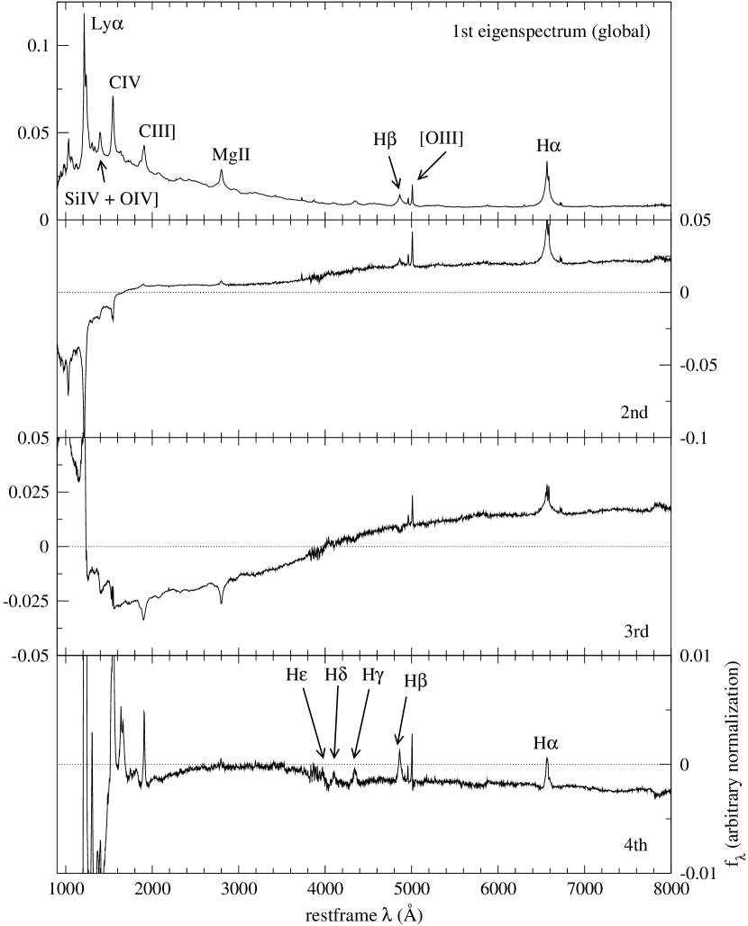
Figure 1: The first 4 eigenspectra of 16,707 SDSS quasars, in the rest wavelengths $900-8000$ Å. Prominent emission lines are indicated. 

The partial sums of weights (i.e., accumulative weights, where the weights are the eigenvalues of the correlation matrix) in different orders of the global eigenspectra are shown in Table 1. The first eigenspectrum accounts for about 0.56 of the total sample variance and the first 10 modes account for $\approx 0.92$. To account for $\approx 0.99$ of the total sample variance, about $50-60$ modes are required. The first four eigenspectra are shown in Figure 1, and their physical attributes will be discussed below.

4.1 First Global Eigenspectrum: Composite Spectrum

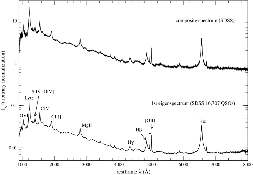
Figure 2: The 1st eigenspectrum of 16,707 SDSS quasars, in the rest-wavelengths $900-8000$ Å. For comparison, the SDSS composite quasar spectrum Vanden Berk et al. (2001) using over 2200 QSOs is also shown. Prominent emission lines are indicated. 

The first eigenspectrum (the average spectrum of the data set) reveals the dominant broad emission lines that exist in the range of $\lambda_{rest}=900-8000$ Å. These, presumably Doppler-broadened lines, are common to most quasar spectra. As can be seen in Figure 2, this eigenspectrum exhibits a high degree of similarity with the median composite spectrum Vanden Berk et al. (2001) constructed using over 2200 SDSS quasars, but with lesser noise at the blue and red ends, probably due to the larger sample used in this analysis.

4.2 Second Global Eigenspectrum: Host-Galaxy Component

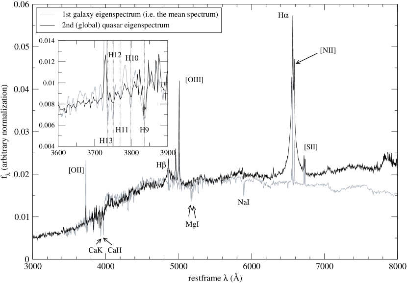
Figure 3: Comparison of the global quasar eigenspectrum of this work with the 1st eigenspectrum (i.e., the mean spectrum) of the SDSS galaxies ($\approx 170,000$ galaxy spectra, from Yip et al. 2004) in the rest-wavelengths $3000-8000$ Å. Not only the major emission lines and absorption lines noted in the graph are found in both cases, the “bumps and wiggles” in the continua also exhibit similarities. The inset shows the spectral region near the hydrogen absorption lines. 

The 2nd eigenspectrum shows a striking similarity in the optical region ($\lambda_{rest}\geq 3500$ Å) with the 1st galaxy eigenspectrum (i.e., mean spectrum) from the SDSS galaxies (of $\approx 170,000$ galaxy spectra; Yip et al. 2004). Figure 3 shows a comparison between the two. Besides the presence of the Ca K and Ca H lines and the Balmer absorption lines as reported previously in the composite quasar spectrum, the Mg I triplet (which appears to be composed of two lines because of the limited resolution, i.e., Mg I$\lambda$5169+$\lambda$5174, and Mg I$\lambda$5185) is also seen in this mode. The presence of the Balmer absorption lines (see the inset of Figure 3) implies the presence of young to intermediate stellar populations near the nuclei (because of the SDSS 3″  spectroscopic fiber). The main differences between the quasar 2nd eigenspectrum and the galaxy mean spectrum lie in the Balmer lines H$\alpha$ and H$\beta$, which are, as expected, Doppler-broadened for the QSO spectra. The quasar eigenspectrum also has a redder continuum, meaning that if this eigen-component represents all contributions from the host-galaxies, the galaxies would be of earlier spectral type than the average spectral type in the SDSS Main galaxy sample.

Our ability to detect significant host-galaxy features in this eigenspectrum triggers an important application, that is, the removal of the host-galaxy contributions from the quasar spectra. The properties the host-galaxies of quasars have recently attracted interest (e.g., Bahcall et al. 1997, McLure et al. 1999, McLure et al. 2000, Nolan et al. 2001, Hamann et al. 2003), mainly because of their obvious relationship with the quasars they harbor and the probable co-evolution that happens between them. Therefore, the evolution of massive galaxies, which are believed to be at one time active quasar hosts (see Hamann & Ferland 1999), can also be probed.

On the other hand, narrow emission lines in active galactic nuclei (AGNs) have been considered less useful than broad emission lines as diagnostic tools, because AGNs with prominent narrow lines have low luminosities (see, for example, the discussion in Chapter 10 of Krolik 1999), in which case contributions from the host galaxies may affect both the continuum and the lines, obscuring their true appearances. Hence, the removal of host-galaxy components can potentially fix the narrow emission lines and reveal their true physical nature. Preliminary results (Vanden Berk et al. 2004, in prep.) show that it is possible to remove the galaxy continuum in the lower-redshift quasars in the SDSS sample. Related issues such as the effects on the broad and narrow emission lines from such a removal procedure are beyond the scope of this paper and are currently being studied.

The second mode also shows slight anti-correlations between major broad emission lines which exist in $\lambda_{rest}$ smaller and larger than $\approx 2000$ Å  (see Figure 1).

4.3 Third Global Eigenspectrum: UV-Optical Continuum Slope

The change of the continuum slope, with a zero-crossing (i.e., a node) at around 3990 Å, dominates this global eigenspectrum. The optical continuum appears to be galaxy-like, but not as much as the 2nd global eigenspectrum. For example, in this component the [O II]$\lambda$3728 is missing, and the nebular lines are generally weaker. The node at $\approx 4000$ Å  is in partial agreement with the 2nd principal component of 18 low-redshift ($z<0.4$; BALQSOs excluded) quasar spectra Shang et al. (2003), which showed the UV-optical continuum variation (except the node is at $\approx 2600$ Å). This particular wavelength (4000 Å) marks the modulation of the slope between the UV and the optical regions. One related effect is the “ultra-violet excess”, describing the abrupt rise of quasar flux densities from about 4000 Å  to 3500 Å. This observed excess flux was suggested to be due to the Balmer continuum Malkan & Sargent (1982), as there seem to be no other mechanisms which can explain this wavelength coincidence. In Malkan & Sargent’s work, an exact wavelength for this onset was not clear. The node at $\approx 4000$ Å  can serve the purpose of defining that wavelength. Other possible physical reasons for the modulations between the UV and optical continua are the intrinsic change in the quasar continuum (e.g., due to intrinsic dust-reddening) and the stellar light from the host galaxy. There is also a second node located in Ly$\alpha$ showing an anti-correlation between the continua blueward and redward of the Ly$\alpha$. Since the number of quasars with spectroscopic measurements in the vicinity of Ly$\alpha$ is much smaller than those with measurements in the UV-optical regions that are redward of Ly$\alpha$, the significance of this anti-correlation is less than that of the UV-optical continuum variation in this eigenspectrum.

4.4 Fourth Global Eigenspectrum: Correlations of Balmer Emission Lines

This mode shows the correlations of broad emission lines, namely, Ly$\alpha$, C IV, Si IV+O IV$]$, C III$]$, Mg II, $[$O III$]\lambda$5008 and also the Balmer emission lines H$\alpha$, H$\beta$, H$\gamma$, H$\delta$ and H$\epsilon$. These are in partial agreement with the 3rd eigenspectrum of Shang et al., in which emission lines C III$]$, Mg II, H$\alpha$, H$\beta$ are found to be involved. It seems natural that these Balmer lines are correlated, as presumably they are formed coherently by some photo-ionization processes. However, it is not known why they appear in this low-order mode. The fact that C III$]$ and H$\beta$ vary similarly was seen previously Wills et al. (2000), and it was suggested that H$\beta$ and C III$]$ may arise from the same optically-thick disk.

4.5 Higher Orders

By construction, subsequent higher-order eigenspectra show more nodes, causing small modulations of the continuum slope. They also show broad absorption line features. Since quasars with BALs are not the dominating populations in our sample (there are 224 broad absorption line quasars in the 3814 quasars from the SDSS EDR quasar catalog, Reichard et al. 2003), their signatures preferentially show up at higher orders in this global set of eigenspectra. The BAL components are not confined to only one particular mode, but span a number of orders. To investigate the effects of BALQSOs on the global eigenspectra, our approach is to perform the KL transform on our original sample (including BALQSOs) and on the same sample but with the BALQSOs excluded, and make a comparison between them. There are 682 BALQSOs (with balnicity index $>0$) found in our sample according to the BALQSO catalog for the SDSS spectra by Trump et al. (private communication).

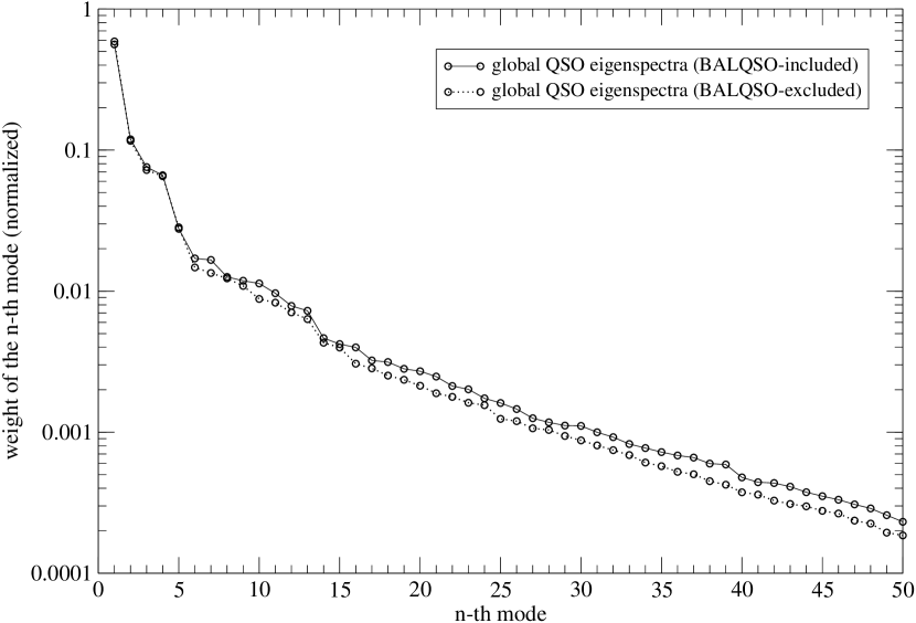
Figure 4: Comparison of the weights at different orders between the BALQSO-included global eigenspectra (i.e., the 16,707 QSOs; solid curve) and the BALQSO-excluded global eigenspectra (dotted curve). Since the BALQSO-included global eigenspectra contain information for features of both typical quasars and broad absorption lines, the weight of each mode is larger than that of the BALQSO-excluded eigenspectra. 

Figure 4 compares the weights at different orders between the BALQSO-included and the BALQSO-excluded global eigenspectra. Since the BALQSO-included global eigenspectra contain information describing both the non-BALQSOs and the BALQSOs, the weight of each mode is larger than that of the BALQSO-excluded eigenspectra. That is, the BALQSO-excluded eigenspectra set is more compact. The magnitude of this offset, however, is small and is apparent only after the 5-th order, which is consistent with the fact that the BALQSOs form a minority population (about $4$ %). This difference is seen to extend to higher orders, implying that the features describing the BALQSOs span a number of higher-order eigenspectra and are not confined to only one particular mode.

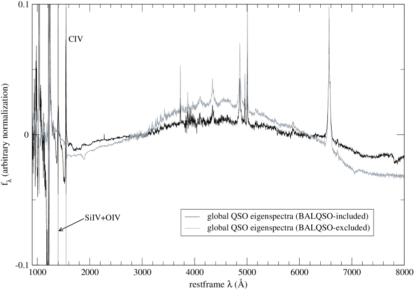
Figure 5: Comparison between the 6th global eigenspectra from the BALQSO-included sample and the BALQSO-excluded one. Absorption features in Si IV+O IV$]$ and C IV exist in the first case and is missing in the latter, as expected. 

A comparison of the 6th global eigenspectrum between the BALQSO included and excluded samples is shown in Figure 5. Absorption features (in this case, in Si IV+O IV$]$ and C IV) are found in the first set of eigenspectra but are missing in the latter. We have to note that the discrepancies in the spectral features of these two sets of eigenspectra attributed to the weight differences are not only confined to the existence or non-existence of BAL absorption troughs as shown here, as the difference in the normalizations between the two can in general also yield different eigenspectra sets. We will leave the discussion of the reconstruction of the BALQSO spectra using eigenspectra till § 5.4 .

4.6 A Non-Unique Set of Eigenspectra: Commonality Analysis

To study the possible evolution and luminosity effects in the quasar spectra, our first step is to investigate whether the set of eigenspectra of a given order derived from quasar spectra in different redshift and luminosity ranges differ. The trace quantity mentioned in § 3 is adopted for these quantitative comparisons.

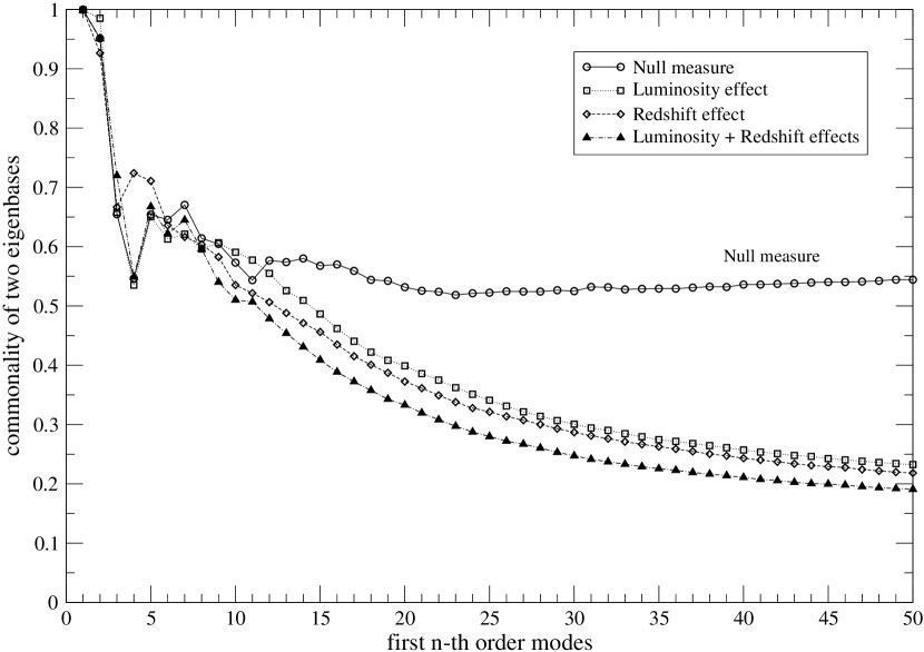
Figure 6: Commonality of two subsamples which are designed to be different from each other mainly due to noise and intrinsic variations (solid line with circles), the additional luminosity effect (dotted line with squares), redshift effect (dashed line with diamonds), and both (dot-dashed line with filled triangles); plotted against the common dimension of the eigenbases (which equals the number of modes constructing each eigenbasis). The commonality departs from unity and progressively drops below the null measure. This means that the two eigenbases under consideration are more disjoint from each other when higher the orders are included.  

As a null measure, two subsamples are chosen with approximately the same redshift and luminosity distributions, such that any differences in the two sets of eigenspectra would be due to noise and the intrinsic variability of the quasars. We fix the rest-wavelengths of this study to be $2000-4000$ Å, and require a full rest-wavelength coverage of the input quasars; redshifts are limited to 0.9 to 1.1. One subsample contains 472 objects (Subsample 1) and the other subsample, 236 objects (Subsample 2). Subsample 2 is, by construction, a subset of the original 472 objects. The reason behind this construction is to ensure a high commonality of the two sets of resultant eigenspectra. They both have luminosities from $-24$ to $-25$, and the actual distributions of redshifts and luminosities are similar. The line on the top in Figure 6 shows the commonality of these two subsamples as we increase the number of eigenspectra forming the subspace. As higher orders of eigenspectra are included in the subspaces, the commonality drops, meaning that the two subspaces become more disjoint. As mentioned above, this disjoint behavior is mainly due to the noise and the intrinsic variability among quasars, both are unlikely to be completely eliminated. At about 20 modes and higher, the commonality levels off, which implies that the eigenspectra mainly contain noise.

With this null measure in place, the differences of our test subsamples are further relaxed to include luminosity effects alone (Subsamples 1 and 3, see Table 2), redshift effects alone (Subsamples 3 and 4), and lastly, both effects combined (Subsamples 1 and 4). The commonalities of these subsamples are overlaid in Figure 6. The first modes constructed in all these subsamples, including the null measure, are always very similar to each other (more than 99 % similar). This shows that a single mean spectrum can be constructed across the whole redshift coverage, which was presumed to be true in many previous constructions of quasar composite spectra. The validity of construction of the mean spectrum in a given sample may seem trivial, but it is not if we take into account the possibility that the quasar population may evolve at different cosmic epochs.

Similar to the null measure, as higher orders are included in the subspaces, the eigenspectra subspaces become more disjoint. In addition, the commonalities in these condition-relaxed cases actually drop below the null measure for orders of modes higher than $\approx 10$. Therefore, the eigenspectra of the same order but derived from quasars of different redshifts and luminosities describe different spectral features. In addition, our results show that both luminosity and evolution effects have detectable influences on the resultant sets of eigenspectra, very much to the same degree (in terms of commonality). In the case of the combined effects, the commonality drops to the lowest value among all cases, as expected.

The actual redshift and luminosity effects found in the quasar spectra will be presented in Sections 6.2 and 6.3. We learn from this analysis that there does not exist a unique set of KL eigenspectra across the whole redshift range, with the number of modes equal or smaller than approximately 10. The implications are twofold. On one hand, the classification of quasar spectra, in the context of the eigenspectra approach, has to be redshift and luminosity dependent. In other words, the weights of different modes are in general different when quasars of different redshifts and luminosities are projected onto the same set of eigenspectra. So, eigenspectra derived from quasars of a particular redshift and luminosity range in general do not predict quasar spectra of other redshifts and luminosities. On the other hand, the existence of the redshift and luminosity effects in our sample can be probed quantitatively by analyzing the eigenspectra subspaces.

5 QSO Eigenspectra in $(M_{i},z)$-bins

KL transforms are performed on subsamples with different redshift and luminosity ranges, that allow us to explicitly discriminate the possible luminosity effects on the spectra from any evolution effects, and vice versa. The constructions of these bins are based on requiring that the maximum gap fraction among the quasars, that is, the wavelength region without the SDSS data, is smaller than 50 % of the the total spectral region we use when applying the KL transforms. The total spectral region, by construction, is approximately equal to the largest common rest-wavelengths of all the quasars in that particular bin. We find that constraining the gap fraction to be a maximum of 50 % improves the accuracy of the gap-correcting procedure for most quasars (see Appendix A for further explanation). As a result, five divisions are made in the whole redshift range $0.08<z<5.13$ (where the quasars of redshifts larger than 5.13 are discarded to satisfy the constraint of 50 % minimum wavelength-coverage in all related luminosity bins), and four in the whole luminosity range $M_{i}=(-30,-22)$. These correspond to ZBIN 1 to 5 and the $M_{i}$ bins A to D for the redshift and luminosity subsamples respectively. In the following, we denote each subsample in a given luminosity and redshift range, for example, the bin A4. Such divisions are by no means unique and can be constructed according to one’s own purposes, but we find that important issues such as the correlation between continua and emission lines remain unchanged as we construct bins with slightly different coverages in redshift, in luminosity and in the total rest-wavelength range. The actual rest-wavelength range and the number of spectra in each bin are shown in Table 3, which also lists the fractions of QSOs in each bin that are targeted either in the quasar color-space Richards et al. 2002a or solely by the Serendipity module. While the majority of the quasars from most of the bins are targeted by using the multi-dimensional color-space, in which the derived eigenspectra are expected to be dominated the intrinsic quasar properties, there is one bin (C4) in which most quasars are targeted by the Serendipity module. In principle, the eigenspectra in the latter case will represent the properties of the serendipitous objects and lack a well motivated color distribution.

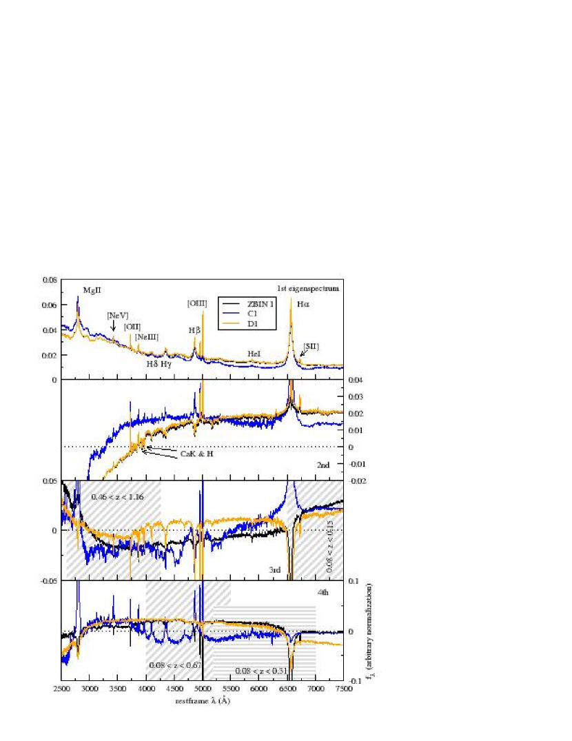
Figure 7: The first 4 orders of ($M_{i},z$)-binned eigenspectra for the subsample ZBIN 1. The shaded areas correspond to the local spectral properties as found in the 2nd local eigenspectra sets using wavelength-selected quasar spectra. (Lowered Resolution)

In general for all $(M_{i},z)$-bins, the first 10 modes or less are required to account for more than 92 % of the variances of the corresponding spectra sets (Table 4). In the iterated calculation of the $(M_{i},z)$-binned eigenspectra, the first 50 modes are used in the gap correction. The first 4 orders of eigenspectra of each ($M_{i},z$)-bin are shown in Figures 7 $-$ 11, arranged in 5 different redshift ranges. In each figure, eigenspectra of different luminosities are plotted along with the ones which are constructed by combining all luminosities (shown in black curves). By visual inspection, the eigenspectra in different orders show diverse properties for each $(M_{i},z)$-bin. In the following, properties associated with different orders are extracted by considering all $(M_{i},z)$-bins generally. Eigenspectra which are distinct from the average population will be discussed separately.

5.1 First $(M_{i},z)$-Eigenspectra: Composite Spectra

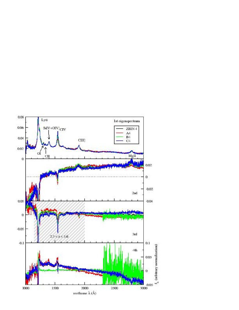
Figure 10: The first 4 orders of ($M_{i},z$)-binned eigenspectra for the subsample ZBIN 4. The meaning of the shaded spectral region is explained in the caption of Figure 7 and § 8.4. (Lowered Resolution)

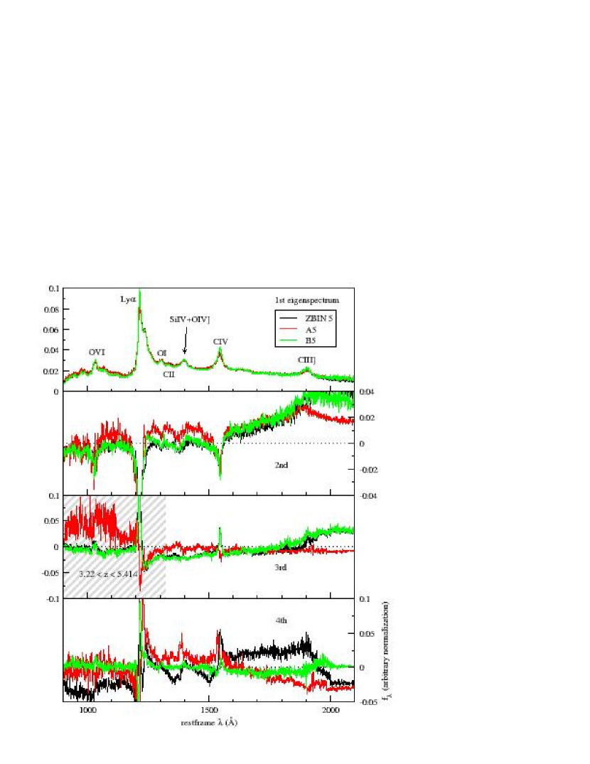
Figure 11: The first 4 orders of eigenspectra of the subsample ZBIN 5. The meaning of the shaded spectral region is explained in the caption of Figure 7 and § 8.4. (Lowered Resolution)

As in the global case, the lowest-order eigenspectra are simply the mean of the quasars in the given subsamples. For every redshift bin, the first eigenspectrum shows approximately a power-law shape (either a single or broken power-law), with prominent broad emission lines. Different luminosity bins show differences in the overall spectral slopes to various degrees. In every redshift range, the spectra of higher-luminosity quasars are bluer than their lower luminosity counterparts. For example, C1 (Figure 7; $M_{i}=-26--24$) shows a harder spectral slope blueward of $\approx 4000$ Å  than that of D1 ($M_{i}=-24--22$). However, for the higher redshift ($z=2.06-5.13$) quasars, e.g., in ZBIN 4 (Figure 10) and 5 (Figure 11), the difference in spectral slope seems to be confined mainly to changes in the flux densities blueward of Ly${\alpha}$.

5.2 Second $(M_{i},z)$-Eigenspectra: Spectral Slopes

The 2nd mode in every $(M_{i},z)$-bin has one node at a particular wavelength. This implies that the linear-combination of the first 2 modes changes the spectral slope. This is similar to the galaxy spectral classification by the KL approach Connolly et al. (1995), in which the first two eigenspectra give the spectral shape.

For the lowest redshift bin (ZBIN 1; Figure 7), the node of the second eigenspectrum occurs at about 3850 Å  for the lower luminosity QSOs (D1), but at $\approx 3300$ Å  for the higher luminosity ones (C1). Possible physical reasons underlying the modulation of the UV-optical slopes were discussed previously in § 4.3. Interestingly, the luminosity averaged 2nd eigenspectrum (black curve) in this redshift range also shows galactic features (as found for the 2nd global eigenspectrum). The continuum redward of $\approx 4000$ Å  is very similar to that in galaxies of earlier-type. Absorption lines Ca K and Ca H, and the Balmer absorption lines H 9, H 10, H 11 and H 12 are seen in the lower-luminosity bin D (and are not present in the higher-luminosity bin C, hence a luminosity dependent effect is implied).

5.3 Third $(M_{i},z)$-Eigenspectra: Anti-correlation between Fe II (UV) and optical continuum around H$\beta$

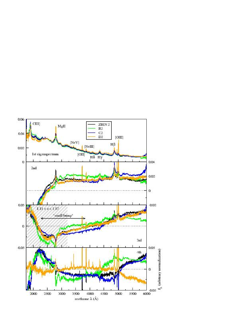
Figure 8: The first 4 orders of ($M_{i},z$)-binned eigenspectra for the subsample ZBIN 2. The meaning of the shaded spectral region is explained in the caption of Figure 7 and § 8.4. (Lowered Resolution)

In addition to the finer-modulation of the continuum slope provided by the 3rd eigenspectrum compared with the 2nd mode, in the redshift range $0.53<z<1.16$ (ZBIN 2; Figure 8), averaging over all luminosities, this mode shows a strong anti-correlation between the quasi-continuum in the Fe II (UV) regions around Mg II (the “small bump”, with its estimated location indicated in the 3rd eigenspectrum in Figure 8) and the continuum in the vicinity of H$\beta$. Around the H$\beta$ emission, the continuum is blended with the Fe II optical blends, the H$\delta$, H$\gamma$ and [O III] lines. The wavelength bounds are found to be $\approx 2120-4040$ Å  for the Fe II ultraviolet blends and $\approx$ 4050 Å  upward (to $\approx$ 6000 Å, which is the maximum wavelength of this redshift bin) for the optical continuum around H$\beta$. This appears to support the calculations that strong Fe II optical emissions require a high optical depth in the resonance transitions of the Fe II (UV) Netzer & Wills (1983); Shang et al. (2003), hence a decrease in the strength of the latter. The actual wavelengths of the nodes bounding the Fe II (UV) region are shown in Figure 8. For brighter quasars (B2), the small bump is smaller ($\approx 2120-3280$ Å) than that found in fainter QSOs.

5.4 Reconstructing BALQSOs with $(M_{i},z)$-eigenspectra

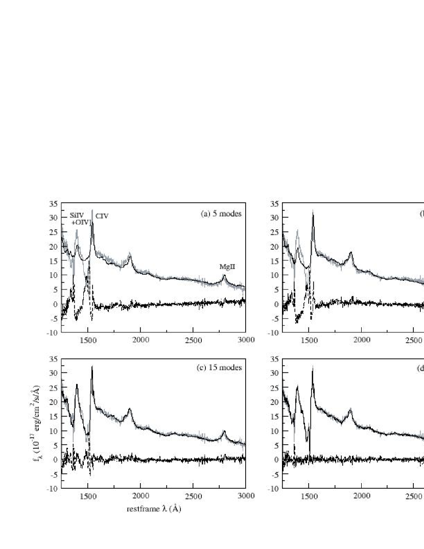
Figure 12: KL-reconstructed spectra (black solid) of a quasar spectrum (gray) with broad absorption features in C IV and Si IV (SDSS J110041.19+003631.9, classified as HiBAL according to Reichard et al. 2003) using the first (a) 5 modes (b) 8 modes (c) 15 modes (d) 50 modes, where the eigenspectra are constructed from the ($M_{i},z$)-bin B3. The bottom dashed curves are the residuals. The broad absorption features span a number of higher-order modes. The observed spectrum is not smoothed. (Lowered Resolution)

To examine the intrinsic broad absorption line features in the $(M_{i},z)$-binned eigenspectra, we study the reconstructed spectra using different numbers of eigenspectra. Figure 12 shows one of the EDR BAL quasars (Reichard et al. 2003) found in the bin B3, and its reconstructed-spectra using different numbers of eigenspectra. This HiBAL (defined as having high-ionization broad absorption troughs such as C IV) quasar is chosen for its relatively large absorption trough in C IV for visual clarity. The findings in the following are nonetheless general. The first few modes ($\stackrel{{\scriptstyle<}}{{{}_{\sim}}}8$ for this spectrum) are found to fit mainly the continuum, excluding the BAL troughs. With the addition of higher-order modes the intrinsic absorption features (in this case, in the emission lines C IV and Si IV) are gradually recovered. Some intrinsic absorption features are found to require $\approx 50$ modes for accurate description, as was found in the global eigenspectra (§ 4.5). We should note that in the reconstructions using different numbers of modes; the same normalization constant is adopted (meaning the eigencoefficients are normalized to $\sum_{m=1}^{50}a_{m}^{2}=1$). Clearly, a different normalization constant in the case of reconstructions using fewer modes (e.g., Figure 12a) will further improve the fitting in the least-squares sense.

While the fact that a large number of modes are required to reconstruct the absorption troughs probably suggests a non-compact set of KL eigenspectra (referring to those defined in this work) for classifying BAL quasars, the appropriate truncation of the expansion at some order of eigenspectra in the reconstruction process will likely lead to an un-absorbed continuum, invaluable to many applications. The proof of the validity of such a truncation will require detailed future analyses. One method is to construct a set of eigenspectra using only the known BAL quasars in the sample and to make comparisons between that and our current sets of eigenspectra. By comparing the different orders of both sets of eigenspectra we may be able to recover the BAL physics. We expect that this separate set of BALQSO-eigenspectra will likely reduce the number of modes in the reconstruction, which is desirable from the point of view of classification.

5.5 KL-reconstructed Spectra

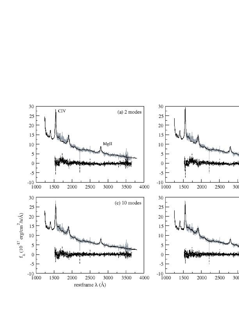
Figure 13: KL-reconstructed spectra (black solid) of an example quasar spectrum (gray) (SDSS J015214.54+131532.0) using the first (a) 2 modes (b) 3 modes (c) 10 modes (d) 20 modes, where the eigenspectra are constructed from the ($M_{i},z$)-bin C3. The bottom dashed curves are the residuals. The observed spectrum is not smoothed. (Lowered Resolution)

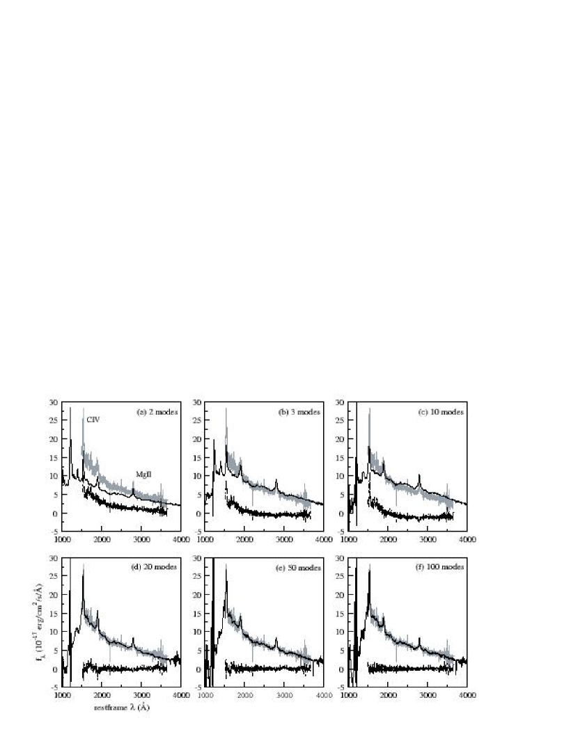
Figure 14: KL-reconstructed spectra (black solid) of the same quasar spectrum (gray) as in Figure 13 using the first (a) 2 modes (b) 3 modes (c) 10 modes (d) 20 modes (e) 50 modes and (f) 100 modes of the global eigenspectra. The bottom dashed curves are the residuals, and the observed spectrum is not smoothed. (Lowered Resolution)

Reconstructions of a typical non-BAL quasar spectrum are shown in Figure 13, using from (a) 2 to (d) 20 orders of eigenspectra. This particular quasar is in the $(M_{i},z)$-bin C3. The bottom curve in each sub-figure shows the residuals from the original spectrum. The first 10 modes are sufficient for a good reconstruction. The reconstructions of the same quasar spectrum but using the global set of eigenspectra are shown in Figure 14, from (a) 2 modes to (f) 100 modes. To obtain the same kind of accuracy, more eigenspectra are needed in the global case; in this case about 50 modes. This is not surprising as the global eigenspectra must account for the intrinsic variations in the quasar spectra as well as any redshift or luminosity evolutions.

There are, therefore, two major factors we should consider when adopting a global set of quasar eigenspectra for KL-reconstruction and classification of quasar (instead of redshift and luminosity dependent sets). First, we need to understand and interpret about $10^{2}$ global eigenspectra. This is significantly larger than found for galaxies (2 modes are needed to assign a type to a galaxy spectrum according to Connolly et al. 1995). This is a manifestation of the larger variations in the quasar spectra. Second, the “extrapolated” spectral region, $\lambda_{rest}<1520$ Å , in Figure 14 (which is the rest-wavelength region without spectral data) show an unphysical reconstruction even when 100 modes are used, although this number of modes can accurately reconstruct the spectral region with data. This agrees with the commonality analysis in § 4.6, that there are evolutionary and luminosity effects in the QSOs in our sample. As such, eigenspectra derived in a particular redshift and luminosity range are in general not identical to those derived in another range.

The accuracy of the extrapolation in the no-data region using the KL-eigenspectra remains an open question for the $(M_{i},z)$-bins. It will be an interesting follow-up project to confront the repaired spectral region with observational data, which ideally cover the rest-wavelength regions where the SDSS does not. For example, UV spectroscopic observations using the Hubble Space Telescope.

6 Evolutionary and Luminosity Effects

6.1 Cross-Redshift and -Luminosity bins Projection

To study evolution in quasar spectra with the eigenspectra, we must ensure that the eigencoefficients reflect the same physics independent of redshift. We know however that the eigenspectra change as a function of redshift (see § 4.6). To overcome this difficulty, and knowing that the overlap spectral region between the two sets of eigenspectra in any pair of adjacent redshift bins is larger than the common wavelength region ($2124-2486$ Å) for the full redshift interval, we study the differential evolution (in redshift) of the quasars by projecting the observed spectra at higher redshift onto the eigenspectra from the adjacent bin of lower redshift. In this way, the eigencoefficients can be compared directly from one redshift bin to the next.

Without the loss of generality, we project the observed quasar spectra in the higher redshift bin (or dimmer quasars for the cross-luminosity projection) onto the eigenspectra which are derived in the adjacent lower-redshift one (or brighter quasars for the cross-luminosity projection). For example, $spec({\bf B3})$ (i.e., the spectra in the $(M_{i},z)$-bin B3) are projected onto $\{$e$({\bf B2})\}$ (the set of eigenspectra from the $(M_{i},z)$-bin B2), and similarly for the different luminosity bins but the same redshift bin. From that, we can derive the relationship between the eigencoefficients and redshift (or luminosity).

6.2 Evolution of the Small Bump

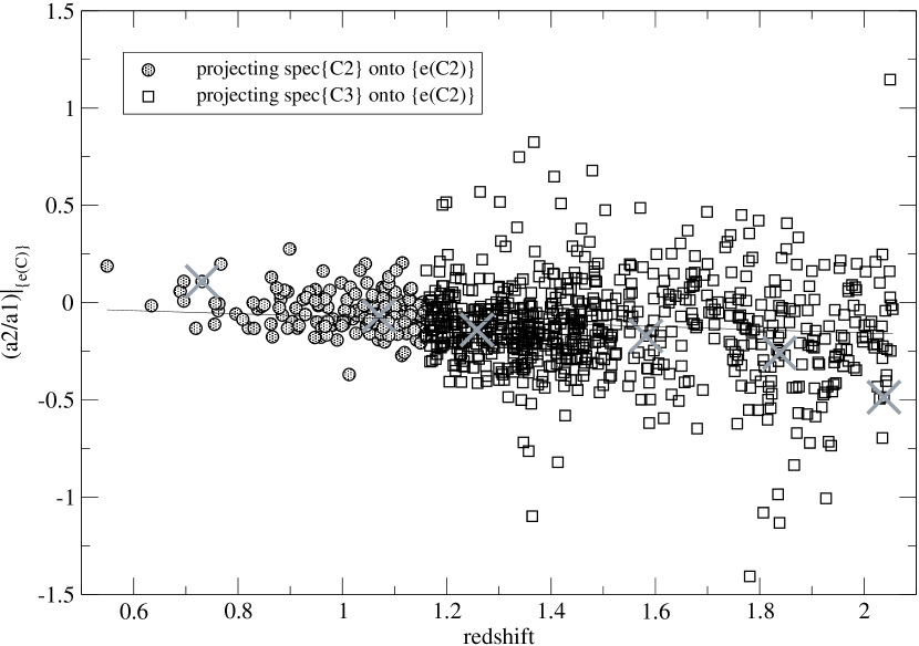
Figure 15: Dependence of $a_{2}/a_{1}$ on redshift, of quasars within the redshift range $0.53-2.06$, and at a fixed luminosity $M_{i}=-25.5\pm 0.1$. The straight line is the regression of the data points: $(a_{2}/a_{1})_{\{e({\bf C2})\}}=-0.0820z+0.0083$. The subscript ${\{e({\bf C2})\}}$ denotes that the eigenspectra are constructed from the subsample ${\bf C2}$. The crosses mark the observed spectra illustrated in Figure 16.

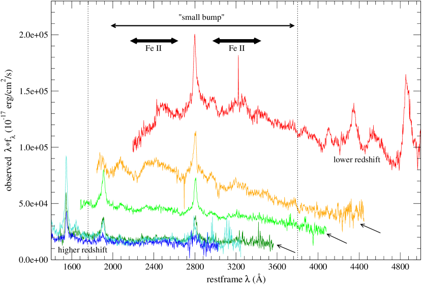
Figure 16: The observed quasar spectra located along the eigencoefficient-redshift relation in Figure 15 in the original flux scales. The evolution of the small bump is evident, in that it is more prominent in the lower-redshift quasar spectra. The vertical dotted lines marked the common wavelength region on which the KL cross-projection is performed. The heavy arrows mark the wavelength regions in which the Fe II emissions are typically found. The spectra are smoothed with a FWHM $=3$ Å  Gaussian smoothing function for easier visualization. (The QSOs are, from the lowest to highest redshifts, SDSS J173052.71+602516.6, SDSS J015352.65-092010.7, SDSS J090934.26+552944.1, SDSS J033801.88+002718.8, SDSS J012858.45+152647.4, SDSS J021552.00-092310.3.)

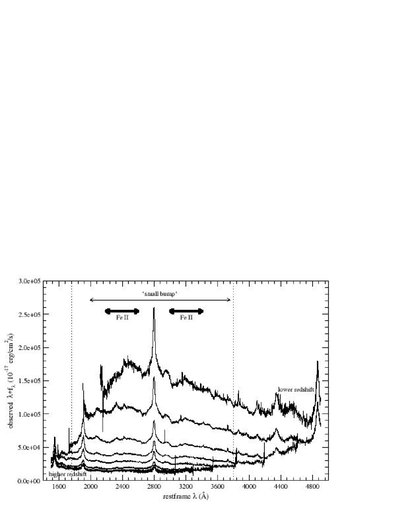
Figure 17: The mean spectra along the redshift trend in Figure 15, from $z=0.6$ to $2.2$ with a bin width in redshift $dz=0.2$. The observed spectra are not smoothed in the calculations of the mean spectra. (Lowered Resolution)

The most obvious evolutionary feature is the small bump present in the spectra at around $\lambda_{rest}\approx 2000$ Å  to $4000$ Å. This feature is mainly composed of blended Fe II emissions ($\approx 2000-3000$ Å, Wills et al. 1985) and the Balmer continuum ($\approx 2500-3800$ Å). When we project quasar spectra of redshifts $1.16-2.06$ (i.e., $spec({\bf C3})$) onto eigenspectra constructed from quasars of redshifts $0.53-1.16$ (i.e., {$e$(C2)}), the coefficients from the second eigenspectrum show a clear trend with redshift, as shown in Figure 15. In this figure, only those quasars with $M_{i}=-25.5\pm 0.1$ are chosen (900 objects), as such the redshift trend does not primarily depend on the absolute luminosities of the quasars. To understand this relation observed spectra are selected along the regression line in Figure 15 (with the locations marked by the crosses) and are shown in Figure 16. The two dotted lines mark the bandpass where the cross-redshift projection is performed. The small bump is found to be present and is prominent in the lower-redshift quasars, whereas it is small and may be absent in the higher-redshift ones. The spectra marked by the arrows in Figure 16 lie relatively close to the regression line. An example of the range of evolution in the small bump as a function of redshift is shown by the remaining 3 spectra which deviate from the regression line. The observed evolution is present independent of which of the spectra we consider. The mean spectra (Figure 17) as a function of redshift, constructed using a bin width in redshift ($dz$) of 0.2, show a similar behavior. Each mean spectrum is calculated by averaging the valid flux densities of all objects in each wavelength bin. The regression of the eigencoefficient-ratios with redshift (with outliers of $a_{2}/a_{1}>1$ removed from the calculation) is

$$(a_{2}/a_{1})_{\{e({\bf C2})\}}=-0.0820z+0.0083\ ,$$ (7)

where the subscript $\{e({\bf C2})\}$ denotes that the eigenspectra are from ${\bf C2}$. The correlation coefficient ($r$) is calculated to be 0.1206 with a two-tailed P-value of 0.00027 (the probability that we would see such a correlation at random under the null hypothesis of $H_{0}:r=0$), as such the correlation is considered to be extremely significant by conventional statistical criteria.

This redshift dependency can be explained by either the evolution of chemical abundances in the quasar environment Kuhn et al. (2001), or an intrinsic change in the continuum itself (which, of course, could also be due to the change in abundances through indirect photo-ionization processes). Green, Forster & Kuraszkiewicz (2001) found in the LBQS that the primary correlations of the strengths of Fe II emission lines are probably with redshift; an evolutionary effect is therefore implied. Kuhn et al. (2001) also supported the evolution of the small bump region $2200-3000$ Å  from high-redshift ($\approx 3-4$) to lower-redshifts ($<0.3$) by comparing two QSO subsamples with evolved luminosities.

As the second mode in the $(M_{i},z)$-binned eigenspectra describes the change in the spectral slope of the sample, the above findings support the idea that the Balmer continuum, as a part of the small bump, changes with redshift. To further understand this effect, the 3rd eigenspectrum in C2 is taken into consideration, which presumably describes the iron lines (see § 5.3). We find that the third eigencoefficient-ratio $a_{3}/a_{1}$ also shows a slight redshift dependency (not shown) with the regression relation (with outliers of $a_{3}/a_{1}>1$ removed from the calculation, resulting in 901 objects)

$$(a_{3}/a_{1})_{\{e({\bf C2})\}}=0.0478z-0.2063$$ (8)

and the correlation coefficient is calculated to be 0.0030 with a two-tailed P-value of 0.93, which is considered to be not statistically significant.

While the strength of this effect shown by the two ratios are of similar magnitude (0.0820 versus 0.0478), the difference in their correlation coefficients implies that the sample variation is much greater in the ratio $a_{3}/a_{1}$ than $a_{2}/a_{1}$. The non-trivial value of the regression slope in the case of $a_{3}/a_{1}$ agrees with the change in shape of the observed line profiles in the small bump regions seen in the local wavelength level (smaller in width than what is expected in the continuum change) with redshift. In conclusion, this implies that there exists the possibility of an evolution in iron abundances but with a larger sample variation compared with that for the continuum change.

To our knowledge, our current analysis is the first one without invoking assumptions of the continuum level or a particular fitting procedure of the Fe II blends that finds an evolution of the small bump; directly from the KL eigencoefficients. Because of the large sample size, the conclusion of this work that the small bump evolves is drawn from spectrum-to-spectrum variation independent of the luminosity effect, in contrast to the previous composite spectrum approaches Thompson et al. (1999), in which the authors found that the composite spectra in two subsamples with mean redshifts $<z>=3.35$ and $<z>=4.47$, and that from the Large Bright Quasar Survey of lower redshifts ($<z>\sim 0.8$) are similar in the vicinity of Mg II and hence did not suggest the existence of a redshift effect. The variation of the small bump with redshift is further confirmed with the study of composite quasar spectra of the DR1 data set (Vanden Berk et al., in preparation). At this point we make no attempt to quantitatively define and deblend the Fe II optical lines and the Balmer continuum, as that would be beyond the scope of this paper. It is a well-known and unsolved problem to identify the true shape of total flux densities due to the Fe II emission lines. This difficulty arises because there are too many Fe II lines to model and they form a quasi continuum.

6.3 Luminosity Dependence of Broad Emission Lines

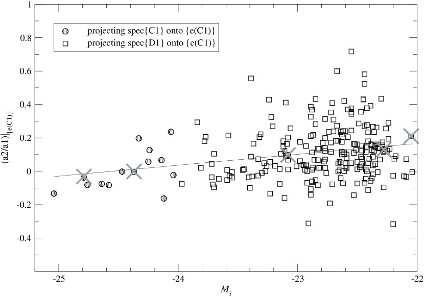
Figure 18: Dependence of $a_{2}/a_{1}$ on the $i$-band absolute luminosity, of quasars with fixed redshifts ($z=0.4\pm 0.02$). The regression line is: $(a_{2}/a_{1})_{\{e({\bf C1})\}}=0.0643M_{i}+1.5797$. The crosses mark the observed spectra plotted in Figure 19a.

Luminosity effects on broad emission lines can also be probed in a similar way to the cross-redshift projection. One prominent luminosity effect is found by projecting $spec({\bf D1})$ onto $\{e({\bf C1})\}$. These samples have the same redshift range but different luminosities (for D1, $M_{i}=(-24,-22)$ and for C1, $M_{i}=(-26,-24)$). Figure 18 shows the eigencoefficient $(a_{2}/a_{1})_{\{e({\bf C1})\}}$ as a function of absolute luminosity, with redshifts fixed at $z=0.4\pm 0.02$ (235 quasars). The ratio of the first 2 eigencoefficients decreases with increasing quasar luminosity. The regression line (with outliers of $a_{2}/a_{1}>1$ removed from the calculation) is

$$(a_{2}/a_{1})_{\{e({\bf C1})\}}=0.0643M_{i}+1.5797\ ,$$ (9)

with a correlation coefficient of 0.2305 with an extremely significant two-tailed P-value of 0.0003.

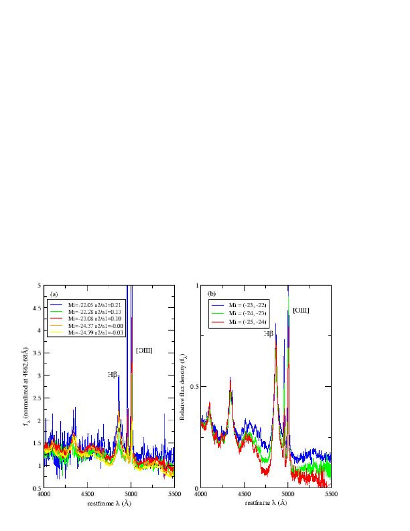
Figure 19: (a) The $H{\beta}$ region of spectra located along the regression line for $(a_{2}/a_{1})_{\{e({\bf C1})\}}$ versus $M_{i}$ (marked with crosses in Figure 18). The spectra are normalized by the continuum flux density at $\lambda=4862.68$ Å  and smoothed with a FWHM $=3$ Å  Gaussian smoothing function. For decreasing $a_{2}/a_{1}$ ratio, i.e., for brighter quasars, the emission line equivalent widths typically decrease. (The QSOs are, starting from the brightest, SDSS J013418.19+001536.6, SDSS J010342.73+002537.2, SDSS J011310.38-003133.1, SDSS J093409.17+023237.0, SDSS J092011.60+571718.2.) (b) The geometric composite spectra in different absolute luminosity bins with $M_{i}$ ranges from -22 to -25 for the objects in Figure 18. (Lowered Resolution)

Along this luminosity trend, the equivalent widths of emission lines such as H$\beta$ and $[$O III$]$ lines are found to decrease typically, as a function of increasing absolute magnitude $M_{i}$ (as shown in the spectra in Figure 19a). This is the Baldwin (1977) effect. We note that the host-galaxy may come into play in this case (at low redshifts and low luminosities). The geometric composite spectra of different luminosities within the range from $-22$ to $-25$ are shown in Figure 19b, in which a spectral index of $\alpha_{\nu}=-0.5$ for the continua is assumed. The Baldwin effect for the emission lines is also present.

In the highest redshift bins, the Baldwin effect can be found in the first and the second eigenspectra. Figure 10 shows that the addition (with positive eigencoefficients) of the first two eigenspectra enhances the flux density around 1450 Å  and reduces the equivalent width of C IV. Ly$\alpha$ and other major BELs are also shown to be anti-correlated with the continuum flux. Hence, the Baldwin effect is not limited to the C IV emission line, and is also observed in many broad emission lines (see, for example, a summary in Sulentic et al. 2000). The linear-combination of the first and third modes in this redshift range also shows a similar modulation between the flux density around 1450 Å  and the line equivalent width. This effect is, however, not general for all luminosities, with the third eigenspectrum in C4 showing only a small value in the 1450 Å  flux density.

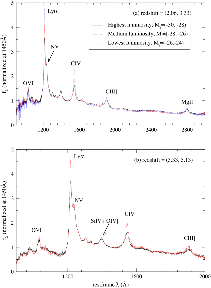
Figure 20: Baldwin effect of the broad emission lines O VI (only in the highest redshifts), Ly$\alpha$, the blended Si IV + O IV$]$, C IV, He II, C III$]$ and Mg II are shown in the redshift ranges (a) $2.06-3.33$ and (b) $3.33-5.13$. In both cases, the 1st eigenspectra in different luminosity ranges are shown, and are normalized at 1450 Å. For N V, the effect appears to be redshift dependent (see § 6.3 for discussions).

The Baldwin effect can also be seen by comparing the first eigenspectra constructed for different luminosity bins. Figure 20 shows the first eigenspectra derived in different luminosities in the second highest redshift bin (i.e., the $(M_{i},z)$-bins A4, B4 and C4, with $2.06<z<3.33$) and the highest one (A5 and B5, with $3.33<z<5.13$). The eigenspectra are normalized to unity at $1450$ Å. The continua for wavelengths approximately greater than 1700 Å  in Figure 20a are not perfectly normalized (which is difficult to define in the first place), but a more careful normalization would only lead to an increase in the degree of the Baldwin effect in the emission lines C III$]$ and Mg II. The Ly$\alpha$ and C IV lines demonstrate the most profound Baldwin effect. Other broad emission lines such as He II$\lambda$1640, C III] and Mg II also exhibit this effect. For the controversial line N V, an “anti-Baldwin” correlation is found at redshifts $2.06-3.33$, such that flux densities are smaller for lower-luminosity quasars. At the highest redshifts in this study ($z=3.33-5.13$, Figure 20b), however, a normal Baldwin effect of N V is found. The redshift dependency in the Baldwin effect for N V may explain the contradictory results found in previous studies (a detection of Baldwin effect of N V in Tytler & Fan 1992; and non-detections in Steidel & Sargent 1991; Osmer et al. 1994; and Laor et al. 1995). While most studies have shown little evidence of the Baldwin effect in the blended emission lines Si IV+O IV$]$, our results support the existence of an effect (though at a much weaker level than that of Ly$\alpha$ and C IV). This is in agreement with two previous works (Laor et al. (1995) which used 14 HST QSOs, and Green, Forster & Kuraszkiewicz (2001) which used about 400 QSOs from the LBQS). In the optical region, at least He II$\lambda$4687 was reported to show the Baldwin effect Heckman (1980); Boroson & Green (1992); Zheng & Malkan (1993).

To further verify that the luminosity dependency of the eigencoefficients implies a Baldwin effect, we also study the eigencoefficients corresponding to the Baldwin effect seen in Figure 20. We find that when $spec({\bf C4})$ are projected onto $\{e({\bf B4})\}$ the luminosity dependency is also seen in the eigencoefficients, with $(a_{2}/a_{1})_{\{e({\bf B4})\}}=0.0327M_{i}+0.8794$ ($r=0.1150$, and an insignificant two-tailed P-value of 0.14) and $(a_{3}/a_{1})_{\{e({\bf B4})\}}=-0.0616M_{i}-1.6948$ ($r=0.2177$, and a very significant two-tailed P-value of 0.0043), both for objects with redshifts within $2.7\pm 0.1$ (161 objects in the case of $a_{2}/a_{1}$ and 166 in that of $a_{3}/a_{1}$).

7 A Spectral Sequence along Eigencoefficients $(a_{1},a_{2})$ in $(M_{i},z)$-bin

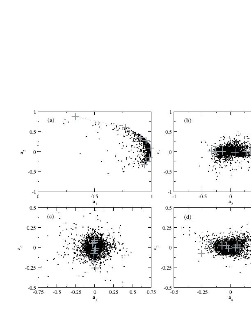
Figure 21: The distributions of the first 5 eigencoefficients of the $(M_{i},z)$-bin B3, in (a) $a_{2}$ versus $a_{1}$ (b) $a_{3}$ versus $a_{2}$ (c) $a_{4}$ versus $a_{3}$ and (d) $a_{5}$ versus $a_{4}$. The crosses mark the observed QSO spectra illustrated in Figure 22. (Lowered Resolution)

Figure 21 shows plots of the first five eigencoefficients of the $(M_{i},z)$-bin B3, where the properties are typical for all $(M_{i},z)$-bins. The eigencoefficients are normalized as: $\sum_{m=1}^{50}a_{m}^{2}=1$. The plot of $a_{2}$ versus $a_{1}$ shows a continuous progression in the ratio of these coefficients which is similar to that found in the KL spectral classification of galaxies Connolly et al. (1995), in which the points fall onto a major “sequence” of increasing spectral slopes. As higher orders are considered, for example $a_{5}$ vs $a_{4}$ (Figure 21d), no significant correlations are observed.

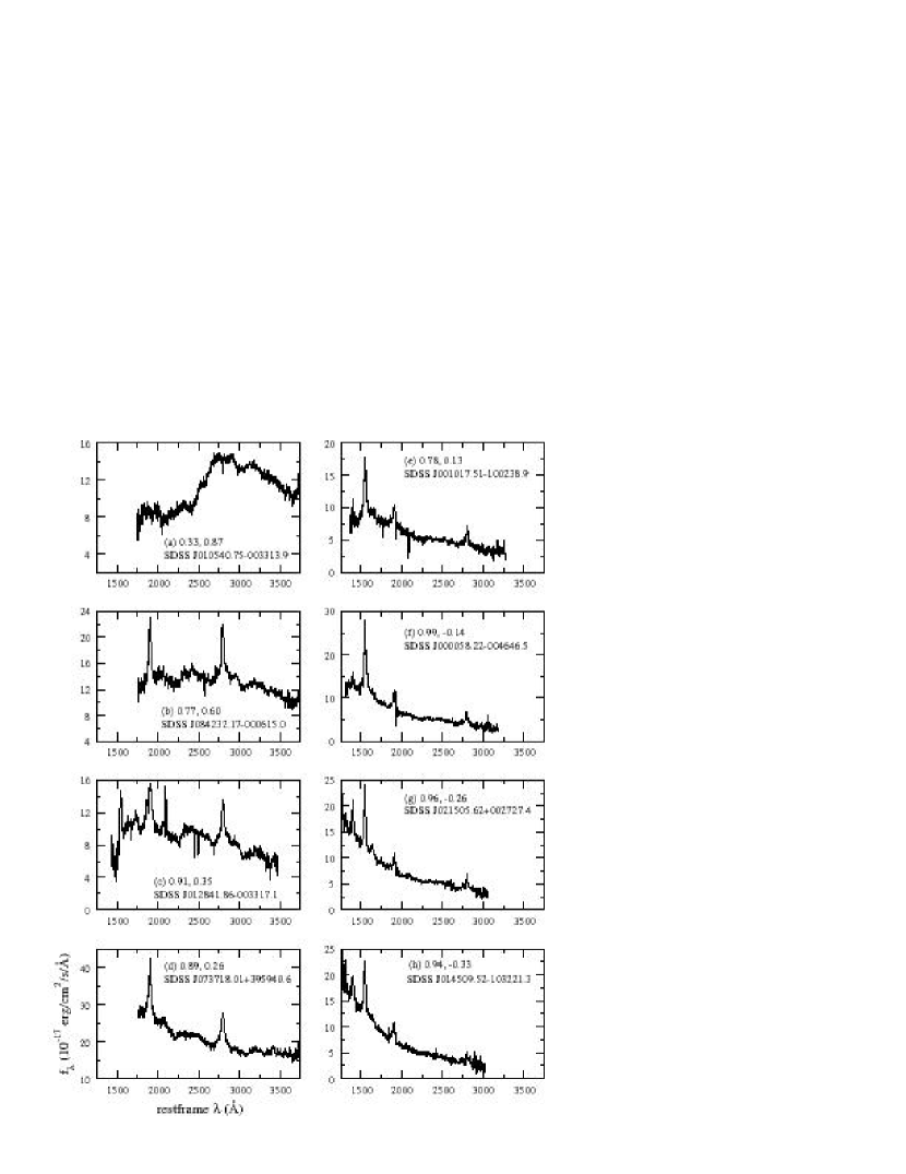
Figure 22: The observed quasar spectra picked along a sequence formed by the first two eigencoefficients $a_{1}$ and $a_{2}$ valued at the two numbers in each figure (see Figure 21 for actual locations of $a_{1}$ to $a_{5}$). Proceeding along the sequence, the spectral slopes of quasars progressively vary from redder to bluer. The spectra are smoothed by a FWHM $=3$ Å  Gaussian smoothing function for easier visualization. The $(M_{i},z)$-bin under consideration is B3. (Lowered Resolution)

Observed quasar spectra are inspected along this trend of $a_{2}$ versus $a_{1}$ (Figure 22). The top of each sub-figure shows the values of $(a_{1},a_{2})$. Along the sequence with decreasing $a_{2}$ values, the quasar continua are progressively bluer. The relatively red continua in Figures 22a to 22c may be due intrinsic dust obscuration Hall et al. (2002). The quasar in Figure 22c is probably a high-ionization BALQSO (HiBAL) according to the supplementary SDSS EDR BAL quasar catalog Reichard et al. (2003). We do, however, emphasize that the appearance of this BALQSO (or any BALQSO in general) in this particular sequence of quasar in the $a_{2}$ versus $a_{1}$ plane does not imply two modes are enough to achieve an accurate classification for a general BALQSO (for the reasons described in § 5.4). The steepness of the spectral slope of this particular BALQSO is the major reason which causes such values of $a_{1}$ and $a_{2}$ eigencoefficients.

On the variations of the emission lines along these major $(M_{i},z)$ sequences, we can appreciate some of the difficulties in obtaining a simple classification concerning all emission lines by inspecting the examples listed in Table 5. The addition of the 2nd eigenspectrum to the 1st, weighted with (signed) medians of the eigencoefficients for all objects in a given sample, broadens some emission lines while making others narrower; a similar effect is seen for the addition of the 3rd eigenspectrum to the 1st, but in two different sets of lines. This shows the large intrinsic variations in the emission line-widths of the QSOs.

8 Local Eigenspectra and Correlations among Emission Lines

One of the utilities of the KL transform is to study the linear correlations among the input parameters, in this case, the pixelized flux densities in a spectrum. Due to possible uncertainties in any continuum fitting procedure in quasar spectra and the fact that no quasar spectrum in our sample completely covers the rest wavelength range $900-8000$ Å, correlations among the broad emission lines are first determined locally around the lines of interest by studying the first two eigenspectra in a smaller restricted wavelength range using the wavelength-selected QSO spectra. This process is then repeated from 900 Å  to 8000 Å. Each local wavelength region is chosen to be $\approx 500-1800$ Å  wide in the restframe. Empirically, we find that at these spectral widths the correlations among broad emission lines can be isolated in the first two eigenspectra without interference by the continuum information (except in the vicinity of Mg II doublet, for which the adjacent strong emission lines are located well beyond the Fe II (UV) region, which can be as broad as $\lambda_{rest}\approx$ $2000-4000$ Å), in contrast to the property of the $(M_{i},z)$-bins in which the 2nd eigenspectra generally describe the variations in the spectral slopes.

The actual procedures to determine the correlations among the strengths of the major emission lines are as follows: $(i)$ in each bin, the eigencoefficients of all objects are computed, and the distribution of the first two eigencoefficients, $a_{2}$ versus $a_{1}$, are divided into several ($\approx 10$) sections within $\pm 1\sigma$ of the $a_{2}$ distribution. In each section the mean eigencoefficients, $<a_{1}>$ and $<a_{2}>$, are calculated (discarding outliers $a_{1}<0$). $(ii)$ Along this trend of mean eigencoefficients, synthetic spectra are constructed by the linear-combination of the first two eigenspectra using the weights defined by the mean eigencoefficients. $(iii)$ The equivalent widths of emission lines in the synthetic spectra are calculated along the trend of mean eigencoefficients, so that the correlations among the strengths of the broad emission lines can be deduced. Linear regression and linear correlation coefficients are calculated from the EW-sequence of a particular emission line relative to that of another line, which is fixed to be the emission line with the shortest wavelength of each local bin. The equivalent widths are calculated by direct summation over the continuum-normalized flux densities within appropriate wavelength windows. From such procedures, the correlations found are ensemble-averaged properties of redshifts and luminosities over the corresponding range, and are physical. Table 6 shows the rest-wavelength bounds, the redshift range, the number of quasar spectra in each bin, and regression and correlation coefficients for each major emission line. The range of the possible restframe equivalent widths (EW_rest) along $(a_{1},a_{2})$ is listed in decreasing $a_{2}$ values. Since the redshifts are chosen such that each quasar spectrum has a full coverage in the corresponding wavelength region, the gap-correcting procedure is implemented to correct only for skylines and bad pixels.

The EW_rest of the emission lines vary at different magnitudes along the $(a_{1},a_{2})$ sequence; some change by nearly a factor of two (e.g., Ly$\alpha$, C IV), while some show smaller changes (e.g., Si IV+O IV$]$, C III$\lambda$1906). Within a single local bin, the rest equivalent widths of some emission lines increase while others decrease along the trend $(a_{1},a_{2})$ with decreasing $a_{2}$ values. These results are the testimonies to the fact that quasar emission lines are diverse in their properties.

We also note that some pairs of emission lines change their correlations as a function of redshift (i.e., different local bins). For example, Mg II is correlated with O III+Fe II(Opt82) in the local bin of $z=1.1-1.87$ but anti-correlated in that of $z=0.46-1.16$. Another example is the $[$S II$]$$\lambda 6718$ and $[$S II$]$$\lambda 6733$ pair. Hence if correlations are interpreted between the emission lines from one local bin with those from an adjacent bin, caution has to be exercised. The uncertainty in the continuum estimation (e.g., the iron contamination in the continuum in the vicinity of Mg II) prevents us from drawing an exact physical interpretation of this phenomenon.

8.1 Francis’s PCs and Boroson & Green’s “Eigenvector-1” in SDSS QSOs

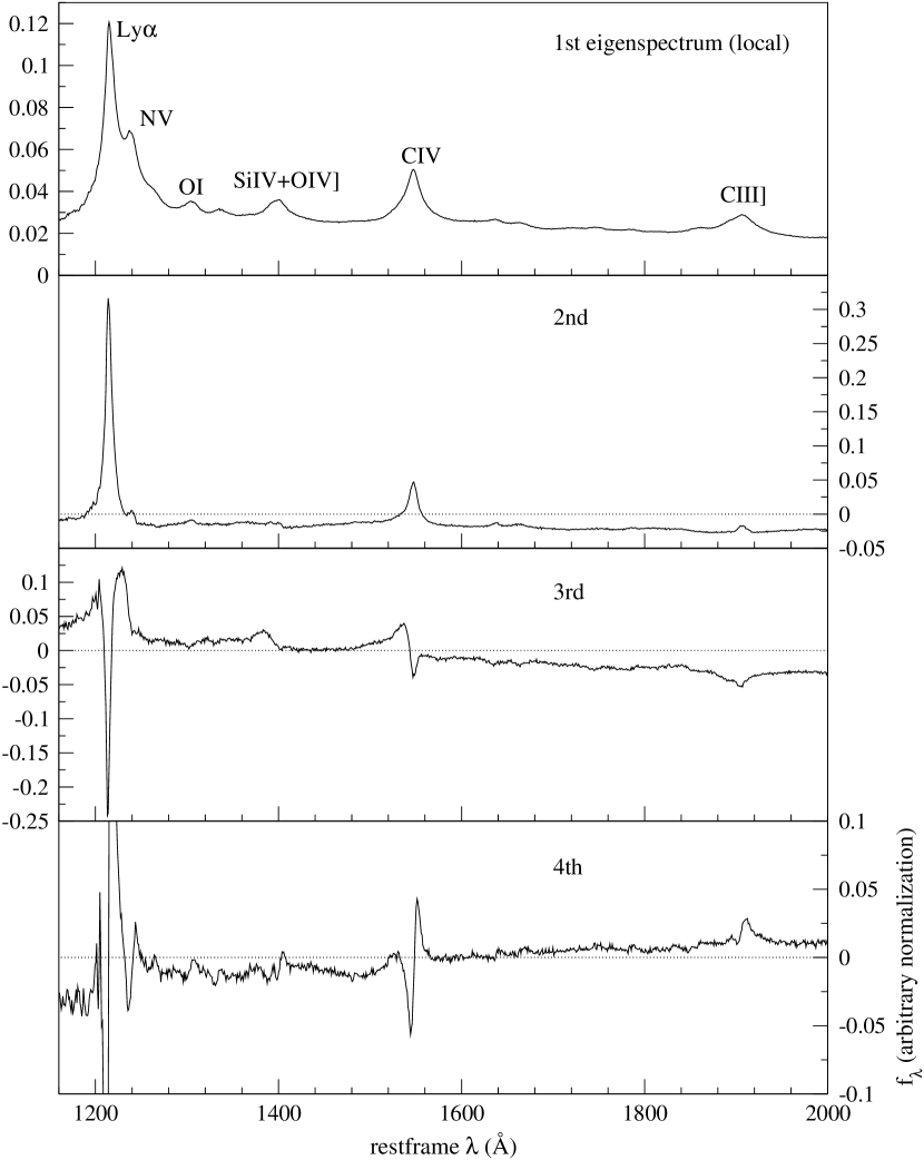
Figure 23: The first 4 orders of locally constructed eigenspectra in the restricted wavelength region $1150-2000$ Å, in which the quasar spectra are chosen to have full wavelength coverage. In this rather narrow rest-wavelength coverage, the emission lines in the 2nd eigenspectrum show the low-velocity core components (i.e., relatively narrower than the first eigenspectrum). The correlations among the relevant board emission lines are probed in the 2nd eigenspectrum. The results agree very well with that by Francis et al. (1992), in, for example, the correlation between Ly$\alpha$ and C IV; and the information about the variations of continuum slopes showing up in the 3rd eigenspectrum.

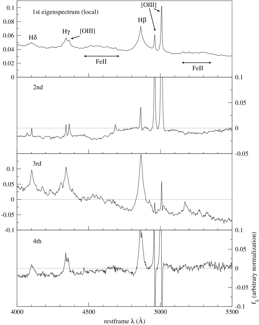
Figure 24: The first 4 orders of locally constructed eigenspectra in the restricted wavelength region $(4000,5500)$ Å, in the vicinity of H${\beta}$. The well-known “Eigenvector-1” (Boroson and Green, 1992), which essentially is the anti-correlation between [O III] and Fe II (optical), are clearly shown in the 2nd eigenspectrum in our work, which is enlarged for easier visualization. The blended H$\gamma$ and [O III] in the 1st eigenspectrum is cleanly split in the 2nd eigenspectrum, which is a nice example showing that the locally constructed 2nd eigenspectrum comprises mainly the line-core components (see also Figure 25). The 3rd eigenspectrum shows prominent contributions from Balmer lines as well as the continuum slope.

Two examples of the locally-constructed eigenspectra are shown in Figures 23 and 24. In Figure 23, the eigenspectra are constructed using wavelength-selected QSO spectra in the rest-wavelengths $1150-2000$ Å  (with $2.3<z<3.6$), so that both Ly$\alpha$ and C IV are covered. Excellent agreement is shown between our eigenspectra and those selected from the Large Bright Quasar Survey in the $1.8<z<2.7$ range Francis et al. (1992). The second eigenspectrum (corresponding to the first principal component in Francis et al.) shows the line-core components of emission lines. In contrast, the 3rd mode (corresponding to their 2nd principal component) shows the continuum slope, with the node located at around 1450 Å. Besides, the addition (with positive eigencoefficient) of the 3rd eigenspectrum to the 1st one enhances the fluxes at shorter wavelengths while increases the C IV blueshift. This supports the finding of a previous study Richards et al. 2002b that C IV blueshift is greater in bluer SDSS QSOs.

At longer wavelengths, the SDSS quasars with redshifts $0.08-0.67$ show the anti-correlation between Fe II (optical) and [O III] (Figure 24), in agreement with the Eigenvector-1 (Boroson & Green 1992). The first two eigenspectra in Figure 24 demonstrate that both the H$\beta$ and the nearby [O III] forbidden lines are anti-correlated with the Fe II (optical) emission lines, which are the blended lines blueward of H$\beta$ and redward of [O III]. In the 3rd local eigenspectrum, the Balmer emission lines are prominent, which was noted previously in the PCA work by Shang et al. (2003). In addition, we find a correlation between the continuum and the Balmer lines in this local 3rd eigenspectrum, so that their strengths are stronger in bluer quasars.

To date, it is generally believed that the anti-correlation between Fe II (optical) and [O III] is not driven by the observed orientation of the quasar. One of the arguments by Boroson & Green was that the [O III]$\lambda$5008 luminosity is an isotropic property. Subsequent studies of radio-loud AGNs have put doubt on the isotropy of the [O III] emissions. Recent work by Kuraszkiewicz et al. (2000), however, showed a significant correlation between Eigenvector-1 and the evidently orientation-independent [O II] emission in a radio-quiet subset of the optically selected Palomar BQS sample, which implies that external orientation probably does not drive the Eigenvector-1. An interesting future project to address this problem is to relate the quasar eigenspectra in the SDSS to their radio properties.

8.2 Weight of Line-Core

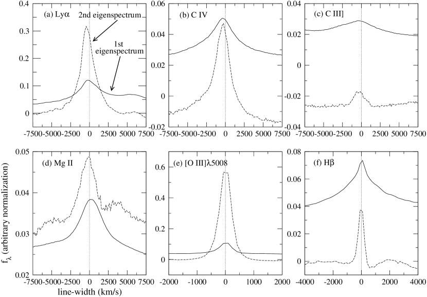
Figure 25: The first (solid line) and the second (dashed line) locally constructed eigenspectra in the regions around (a) Ly$\alpha$ (b) C IV (c) C III$]$ (d) Mg II (e) $[$O III$]$$\lambda$5008 and (f) H$\beta$. The generally narrower second eigenspectrum (except for Mg II, in which the conclusion is complicated by the surrounding Fe II lines) compared with the first one suggests that it mainly carries the line-core (i.e., low radial velocity) information to varies levels.

Enlargements of the first two locally constructed eigenspectra focusing on major broad emission lines are illustrated in Figure 25. Except for the almost perfectly symmetric and zero velocity of the line centers of the 1st and 2nd eigenspectra exhibited by [O III]$\lambda$5008, most broad emission lines do show asymmetric and/or blueshifted profiles. These demonstrate the variation of broad line profiles of quasars and the generally blueshifted broad emission lines relative to the forbidden narrow emission lines. The forbidden lines in the narrow line regions of a QSO are always adopted in calculating the systemic host-galaxy redshift, so the clouds associated with blueshifted BELs probably have additional velocities relative to the host. This line-shift behavior was found in many other studies (see references in Vanden Berk et al. 2001). The behavior of the C IV shift led Richards et al. (2002b) to suggest that orientation (whether external or internal) may be the cause of the effect.

It is also obvious from Figure 25 that the 2nd eigenspectra are generally narrower (except for Mg II, in which the conclusion is complicated by the presence of the surrounding Fe II lines) than their 1st eigenspectra counterparts. The line-widths of the sample-averaged KL-reconstructed spectra using only the first eigenspectrum or the first two eigenspectra are listed in Table 7. The addition of the first two modes, weighted by the medians of the eigencoefficients, causes the widths of 76 % of the emission lines (with FWHM $>1000$ km s^-1) to be narrower than those reconstructed from the first mode only. Hence, most broad emission lines can be mathematically decomposed into broad, high-velocity components and narrow, low-velocity components. Appearing in the second local eigenspectra, the line-widths are thus the most important variations of the quasar broad emission lines. The line-core components were reported by Francis et al. (1992) for C IV and Ly$\alpha$; and Shang et al. (2003) for some major broad emission lines. One nice illustration of the line-core component of the 2nd mode is the splitting of H$\gamma$ and its adjacent [O III] in Figure 24, for they are blended in the 1st mode.

Similar properties may be expected in the 2nd $(M_{i},z)$-binned eigenspectra. Table 5 lists the average FWHM of different linear combinations using the first 3 eigenspectra in constructing some major broad emission lines. Comparatively, for most emission lines the second $(M_{i},z)$-binned eigenspectra do not show as narrow line components as the second eigenspectra, in which the widths of 61 % of the emission lines with FWHM $>1000$ km s^-1 become narrower by adding the 2nd eigenspectrum to the 1st one. This effect is mainly due to the difference in the numbers of quasars, and more importantly, the inclusion of a wider spectral region causes the ordering of the weights of different physical properties to re-arrange. In this case, the spectral slope variations are more important than those of the line-cores. While the 3rd $(M_{i},z)$-binned eigenspectra (weighted by medians of the eigencoefficients of the sample) also do not represent prominent changes in the emission line-cores, except for Ly$\alpha$ and C IV (the FWHM of C IV appears to be larger because the line-core 3rd mode is pointing downward in ZBIN 4), on average the quasar populations with negative 3rd eigencoefficients do show narrower widths for 77 % of the emission lines. Similarly, the 2nd global eigenspectrum does not carry dominant emission line-core components, which are found to be represented more prominently by the 3rd mode (Table 8).

8.3 FWHM-EW Anti-Correlation in BELs: Classification?

The narrower emission features in the 2nd local eigenspectrum compared with the 1st one, and the fact that almost every broad emission line is pointing towards positive flux values in both of these two modes, imply that there is an anti-correlation between FWHMs and the equivalent widths of broad emission lines. In fact, as suggested by Francis et al. (1992), this may form a basis for the classification of quasar spectra in $\lambda_{rest}=1150-2000$ Å, by arranging them accordingly into a sequence varying from narrow, large-equivalent-width to broad, low-equivalent-width emission lines. From the locally constructed eigenspectra, such an anti-correlation is not generally true for every broad emission line as we find that there exists at least one exception: a positive correlation between the FWHM and the EW of Mg II in the local bin of the redshift range $0.46-1.16$. An assumption in these measurements is that the continuum underneath can be approximated by a linear-interpolation across the window $2686-2913$ Å. One complication, however, is the contamination due to the many Fe II emission lines in the vicinity of Mg II, so the true continuum may be obscured. The positive FWHM-EW correlations appear to exist in some other weaker emission lines as well, but the weak strengths of those lines do not permit us to draw definitive conclusions under the current spectral resolution. In conclusion, the FWHM-EW relation can help us to classify most broad emission lines individually, but this relation cannot be used in a general sense, nor does it represent the most important sample variation, if the surrounding continua are included to the extent of the rest-wavelength ranges of the $(M_{i},z)$-binned spectra. Nonetheless, most broad emission lines can be viewed mathematically as the combinations of broad and narrower components. A future study will focus on finding the best physical parameters for classifying the spectra in the wide spectral region, which will be the subject of a second paper. One possible approach is to study the distributions of the eigencoefficients and their relations with other spectral properties (e.g., Francis et al. 1992; Boroson & Green 1992).

8.4 Local Spectral Properties in the $(M_{i},z)$-Eigenspectra

The shapes of the continua and the correlations among the broad emission lines of the second locally constructed eigenspectra are all identified in either the 3rd or the 4th $(M_{i},z)$-binned eigenspectra. We do expect, and it is indeed found to be true, that the local properties of the spectra can be found in the latter, though the ordering may be different. The identifications are marked in Figures 7 $-$ 11 by the redshift ranges of the local eigenspectra, with reference to the luminosity averaged ZBIN eigenspectra. The correlations of broad emission lines are generally found in higher-order $(M_{i},z)$-binned eigenspectra compared with the orders representing the spectral slopes.

9 Summary and Future work

We perform KL transforms and gap-corrections on 16,707 SDSS quasar spectra. In rest-wavelengths $900-8000$ Å, the 1st eigenspectrum (i.e., the mean spectrum) shows agreement with the SDSS composite quasar spectrum Vanden Berk et al. (2001), with an abrupt change in the spectral slope around 4000 Å. The 2nd eigenspectrum carries the host-galaxy contributions to the quasar spectra, hence the removal of this mode can probably prevent the obscuration of the real physics of galactic nuclei by the stellar components. Whether this eigenspectrum is the only one containing galaxy information requires further study. The 3rd eigenspectrum shows the modulation between the UV and the optical spectral slope, in agreement with the 2nd principal component of Shang et al. (2003). The 4th eigenspectrum shows the correlations between Balmer emission lines.

Locally around various broad emission lines, the eigenspectra from the wavelength-selected quasars qualitatively agree with those from the Large Bright Quasar Survey, the properties in the Eigenvector-1 Boroson & Green (1992), and the anti-correlations between the FWHMs and the equivalent widths of Ly$\alpha$ and C IV Francis et al. (1992). The anti-correlation between the FWHM and the equivalent width is found in most broad emission lines with few exceptions (e.g., Mg II is discrepant).

From the commonality analysis of the subspaces spanned by the eigenspectra in different redshifts and luminosities, the spectral classification of quasars is shown to be redshift and luminosity dependent. Therefore, we can either use of order 10 $(M_{i},z)$-binned eigenspectra, or of order $100$ global eigenspectra to represent most (on average 95 %) quasars in the sample. We find that the first two modes can describe the spectral slopes of the quasars in all $(M_{i},z)$-bins under study, which is the most significant sample variance of the current QSO catalog. The simplest classification scheme can be achieved based on the first two eigencoefficients, so that a physical sequence can be formed upon the linear-combinations of the first two eigenspectra. The diversity in quasar spectral properties, and the inevitable different restframe wavelength coverages due to the nature of the survey, increase the sparseness of the data. Hence, higher-order modes enter into the construction of the broad emission lines with the eigenspectra, in contrast to the galaxy spectral classification, in which most emission lines vary monotonically with the spectral slope Connolly et al. (1995). This result is also a manifestation of the high uniformity of galaxy spectra compared with quasar spectra.

We find that BAL features do not only appear in one particular order of eigenspectrum but span a number of orders, mainly higher-orders. This may indicate substantial challenges to the classification of BAL quasars by the current sets of eigenspectra in terms of arriving at a compact description. A separate KL-analysis of the BAL quasars is desirable for studying the classification problem. Nonetheless, the appropriate truncation of the number of eigenspectra in reconstructing a quasar spectrum can in principle lead to an un-absorbed continuum.

We find evolution of the small bump by the cross-redshift KL transforms, in agreement with the quasars from the Large Bright Quasar Survey Green et al. (2001) and in other independent work Kuhn et al. (2001). The Baldwin effect is detected in the cross-luminosity KL transforms, as well as from the mean QSO spectra derived for different luminosities. One implication of these redshift and luminosity effects is that they have to be accounted for in the spectral classification of quasars, consistent with our finding from the commonality analysis.

The high quality of the data allows us to obtain quasar eigenspectra which are generic enough to study spectral properties. Despite the presence of diverse quasar properties such as different continuum slopes and shapes, and various emission line features known for several decades, our analysis shows that there are unambiguous correlations among various broad emission lines and with continua in different windows.

A second paper is being prepared to address the classifications of the DR1 quasars in greater detail. One interesting direction is to relate the current eigenspectra approach to the radio properties of the quasars, so that further discriminations of intrinsic and extrinsic properties can be achieved, for example, the orientation effects on the observed spectra (e.g., Richards et al. 2002b). Another application currently being addressed is the removal of host-galaxy components from the SDSS quasar spectra. In addition, the cross-projections can also be applied to study future larger samples of quasars (e.g., $\approx$ 100,000 at the completion of the SDSS) for possibly new evolution and luminosity effects.

Appendix A KL Gap-Correction in Quasar Spectra

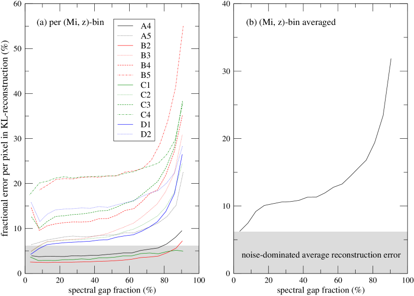
Figure 26: The fractional error of KL-reconstruction in flux density per wavelength bin as a function of the spectral gap fraction in the observed quasar spectra, where in (a) each curve is averaged over all quasars in the corresponding $(M_{i},z)$-bin, and in (b) the curve is averaged over all quasars in all $(M_{i},z)$-bins. The gray region in each is the excluded region due to the average intrinsic noise per wavelength bin.

The construction of the $(M_{i},z)$-bins in this work (§ 5) is performed by constraining the gap fraction to be smaller than 50 % for each spectrum to improve the accuracy of spectral reconstructions using eigenspectra. Here we discuss in detail how this value is arrived at. We artificially mask out (i.e. assign a zero weight) to given spectral intervals and study how well we can reconstruct these “gappy” regions from the eigenspectra Connolly & Szalay (1999). The comparison of the KL-reconstructed spectrum with the original unmasked spectrum gives a direct assessment to the accuracy of the gap-correction procedure. We perform this test for the $(M_{i},z)$-binned quasar spectra from this work. To simulate the effects of un-observed spectral regions due to different rest-wavelength coverage for quasars at different redshifts (the principal reason for gaps in the quasar spectra in our sample), each spectrum in all $(M_{i},z)$-bins is artificially masked at the short- and the long-wavelength ends. The masked spectra are then projected onto the appropriate eigenspectra and the reconstructed spectra are calculated using the first 50 modes. The fractional change in the flux density per wavelength bin (weighted by $w_{\lambda}$), $\sqrt{\sum_{\lambda}w_{\lambda}(f_{\lambda}-f_{\lambda}^{Recon})^{2}}/\sum_{\lambda}w_{\lambda}f_{\lambda}$, between the observed spectrum $f_{\lambda}$ and the reconstructed spectrum $f_{\lambda}^{Recon}$, averaged over all quasar spectra in each bin, are shown in Figure 26a as a function of the spectral gap fraction. The gap fraction is calculated relative to the full restframe wavelength range, a variable for each quasar spectrum. The reconstruction from $50$ modes has an intrinsic error of approximately $6.2$ % (due to the noise present in each spectrum, and the existence of $3.4$ % bad pixels on average for each spectrum), which is estimated by reconstructing the spectra with no artificial gaps. As expected, the difference between the unmasked observed spectrum and the reconstructed spectrum increases gradually with gap fraction.

Averaging over all $(M_{i},z)$-bins (Figure 26b), at a spectral gap fraction of $52.5$ % the mean error in the 50-mode reconstruction is $\approx 11.9$ %, which is $5.7$ % above the noise-dominated average reconstruction error in the flux. While a smaller gap fraction is in principle more desirable, 50 % is chosen to be the upper bound to compromise the fewer $(M_{i},z)$-bins.

In the construction of the global eigenspectra set covering the rest-wavelength range $900-8000$ Å, there are 89 % of the QSOs (Table 9) having spectral gap fractions larger than 50 %. From Figure 26b, we find that a gap fraction larger than $76$ % gives substantial reconstruction errors ($>16.8$ %), implying $\approx 17$ % of the QSOs used in defining the global eigenspectra may be poorly constrained when correcting for the missing data. We stress that in defining the global eigenspectra from the SDSS this is strictly the best estimation that can be made at present, as no SDSS spectroscopic observations are available in the gap regions at the red and the blue ends of the spectrum. The impact of this gap correction is, as expected, wavelength dependent. Wavelengths shortward of $5000$ Å are very well constrained even with the global eigenspectra with less than 1 % of QSOs having gap corrections in excess of 76 % (Table 9). Determining the impact of the gaps and the use of additional spectroscopic observations to complement the SDSS data will be addressed in a future paper.

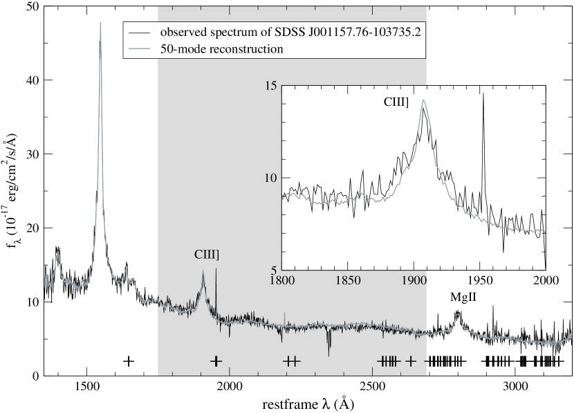
Figure 27: A typical case of the 50-mode reconstruction using the $(M_{i},z)$-binned eigenspectra. The spectrum has a total gap fraction of $56.5$ % including the broad emission line C III$]$. The gray area is the artificially masked spectral region, and the crosses mark the bad pixels in the original spectrum. The fractional reconstruction error per pixel is $12.1$ %. The inset shows the emission line C III$]$ locally.

We also find that quasar broad emission lines can be reconstructed locally using the $(M_{i},z)$-binned eigenspectra with errors that are typically small relative to the noise level. For example, if C III$]$ is masked (over the region of influence $1830-1976$ Å), averaging over all QSOs in the bins B3 and C3, the 50-mode reconstruction error described above is 10.4 %; and for Mg II (over the region of influence $2686-2913$ Å), 11.3 %. For the case in which at least one broad emission line is masked and with a substantial total gap fraction (in our case, C III$]$; and a mean spectral gap fraction of $60.0$ %), the average reconstruction error per pixel is found to be $12.5$ % when averaging over the bins B3 and C3. Figure 27 shows the observed and the reconstructed spectra of an object with a reconstruction error approximately equal to the average value. While the reconstructed continuum has a small difference from the observed continuum, the emission line C III$]$ is reconstructed well, extremely well if considering the fact that the whole region of influence is within the masked region. The actual quality of the reconstruction depends on the individual spectrum and position and size of the gaps.

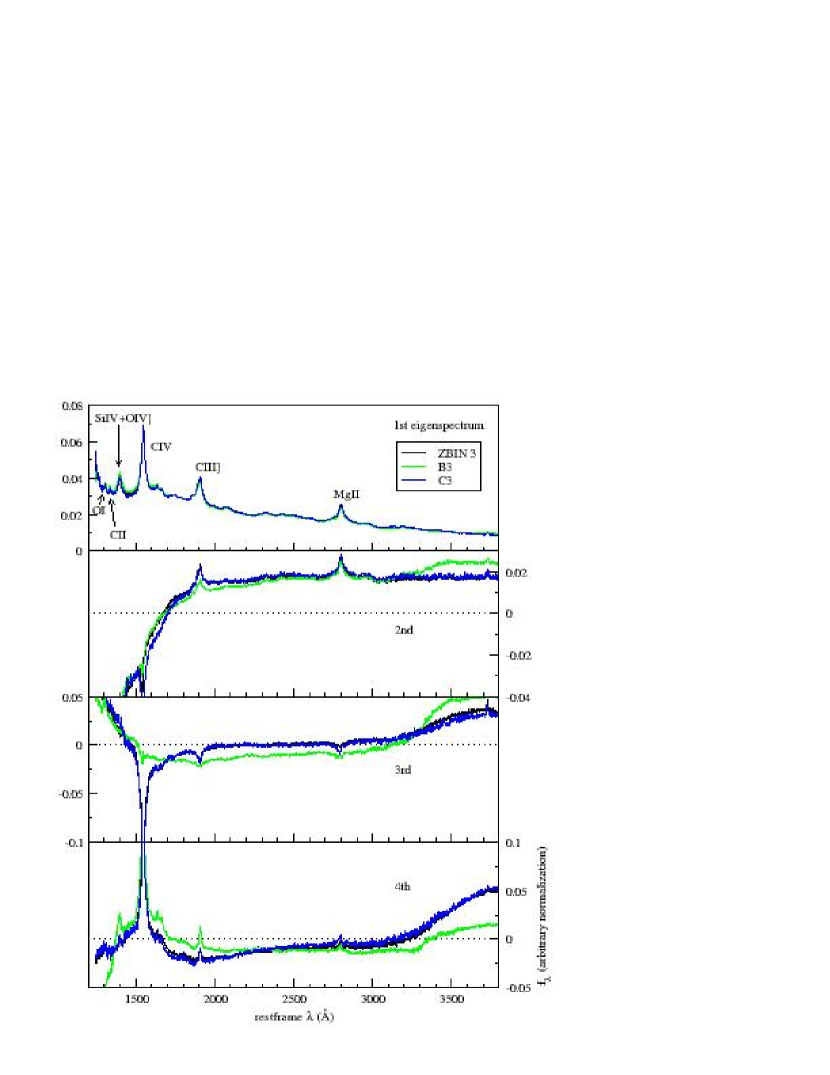
Figure 9: The first 4 orders of ($M_{i},z$)-binned eigenspectra for the subsample ZBIN 3. (Lowered Resolution)

Table 1: The partial sums of weights of the global QSO eigenspectra.

Number of first m-modes: m	Weight
1	0.560887
2	0.680197
3	0.755992
4	0.822280
5	0.849927
8	0.896213
10	0.919394
15	0.953041
20	0.968920
50	0.995680
75	0.998512
100	0.999199

Table 2: The subsamples for performing the commonality analysis on the resultant sets of eigenspectra.

Name	Redshift range	Luminosity range ($M_{i}$)	Number of objects
Subsample 1	0.9 to 1.1	-24 to -25	472
Subsample 2	0.9 to 1.1	-24 to -25	236
Subsample 3	0.9 to 1.1	-25 to -26	442
Subsample 4	1.1 to 1.3	-25 to -26	469

Table 3: The number of QSOs in the $(M_{i},z)$-bins.

	A	B	C	D
	$M_{i}=(-30,-28)$	$M_{i}=(-28,-26)$	$M_{i}=(-26,-24)$	$M_{i}=(-24,-22)$
ZBIN 1: $0.08<z<0.53$			109	1597
$2486-8000$ Å			(95% , 0% )	(81%, 4%)
2: $0.53<z<1.16$		178	2752	1351
$1759-6018$ Å		(94%, 0%)	(79%, 12%)	(30%, 45%)
3: $1.16<z<2.06$		3477	4462
$1242-3800$ Å		(92%, 4%)	(41%, 46%)
4: $2.06<z<3.33$	110	1796	477
$900-3005$ Å	(74%, 0%)	(65%, 11%)	(0%, 61%)
5: $3.33<z<5.13$	85	352
$900-2123$ Å	(94%, 0%)	(75%, 1%)

Table 4: The partial sums of weights of the $(M_{i},z)$-binned QSO eigenspectra.

weight	1 mode	2 modes	3 modes	5 modes	10 modes	15 modes	20 modes	50 modes
ZBIN: 1	0.9284	0.9646	0.9729	0.9836	0.9915	0.9934	0.9942	0.9945
2	0.9317	0.9657	0.9752	0.9815	0.9874	0.9896	0.9905	0.9909
3	0.9232	0.9556	0.9651	0.9763	0.9841	0.9870	0.9880	0.9885
4	0.8737	0.9089	0.9298	0.9455	0.9608	0.9685	0.9719	0.9738
5	0.8122	0.8540	0.8783	0.8986	0.9247	0.9356	0.9398	0.9422
$(M_{i},z)$-bin: A4	0.9134	0.9449	0.9551	0.9663	0.9781	0.9842	0.9866	0.9881
A5	0.8801	0.9076	0.9242	0.9384	0.9555	0.9637	0.9676	0.9699
B2	0.9789	0.9926	0.9958	0.9973	0.9984	0.9989	0.9991	0.9991
B3	0.9474	0.9701	0.9781	0.9859	0.9911	0.9931	0.9938	0.9941
B4	0.8794	0.9115	0.9292	0.9516	0.9673	0.9743	0.9771	0.9787
B5	0.8083	0.8487	0.8718	0.8941	0.9207	0.9314	0.9358	0.9383
C1	0.9893	0.9955	0.9969	0.9981	0.9991	0.9994	0.9995	0.9995
C2	0.9470	0.9709	0.9819	0.9870	0.9921	0.9938	0.9944	0.9947
C3	0.9226	0.9546	0.9631	0.9739	0.9805	0.9832	0.9842	0.9848
C4	0.8365	0.8756	0.8983	0.9191	0.9387	0.9494	0.9539	0.9565
D1	0.9289	0.9640	0.9715	0.9829	0.9908	0.9928	0.9937	0.9941
D2	0.9086	0.9469	0.9586	0.9698	0.9768	0.9797	0.9809	0.9816

Table 5: The average FWHMs of major broad emission lines of the ZBINs QSO eigenspectra.

				FWHM (km s-1)
				(ZBIN)
Percentage of Lines	1st$-$3rd	1st$-$2nd	1st	1st+2nd	1st+3rd
Narrower than 1st mode	77%	40%	$\cdots$	61%	39%
Wider than 1st mode	23%	60%	$\cdots$	39%	61%
Example:						Redshift bin
Ly$\alpha$+N V $(1160,1290)$Å	8999	3343	4405	7918	3116	ZBIN 5
C IV $(1494,1620)$Å	3579	4110	4140	4179	4913	ZBIN 4
C III$]$ $(1830,1976)$Å	5291	5597	5905	6296	6588	ZBIN 4
Mg II $(2686,2913)$Å	4274	4318	4204	4096	4126	ZBIN 3
H$\beta$ $(4050,4152)$Å	1661	2035	1795	1443	1998	ZBIN 1
$[$O III$]$$\lambda 5008$ $(4982,5035)$Å	493	494	495	495	497	ZBIN 1

Table 6: Correlations among major emission lines deduced from the local QSO eigenspectra sets.

Line	$\lambda_{lab}$ (Å)	$(\lambda_{low},\lambda_{upp})$    (Å)	$\lambda_{rest}$ (Å)	$z$ (num. of obj.)	EWrest (Å)	Reg. Coeff.	Corr. Coeff.	P-value
Ly$\beta$+OVI	1025.72+1033.83	$(1012,1055)$	$900-1320$	$3.22-5.414~{}(496)$	$9.08-14.30$	$1.0000$	$1.0000$	0.000000
Ly$\alpha$+NV	1215.67+1240.14	$(1160,1290)$			$74.17-140.28$	$12.6411$	$0.9985$	0.000000
NV	1240.14	$(1230,1252)$			$2.31-1.05$	$-0.2405$	$0.9332$	0.000080
OI+SiII	1304.35+1306.82	$(1290,1318)$			$1.10-2.59$	$0.2833$	$0.9931$	0.000000
Ly$\alpha$+NV	1215.67+1240.14	$(1160,1290)$	$1150-2000$	$2.3-3.6~{}(1277)$	$122.96-65.82$	$1.0000$	$1.0000$	0.000000
NV	1240.14	$(1230,1252)$			$1.87-2.06$	$-0.0032$	$0.9760$	0.000001
OI+SiII	1304.35+1306.82	$(1290,1318)$			$2.40-1.22$	$0.0206$	$0.9999$	0.000000
CII	1335.30	$(1325,1348)$			$0.72-0.67$	$0.0009$	$0.9862$	0.000000
SiIV+OIV$]$	1396.76+1402.06	$(1360,1446)$			$9.12-9.24$	$-0.0021$	$0.9812$	0.000001
CIV	1549.06	$(1494,1620)$			$35.45-17.56$	$0.3129$	$0.9997$	0.000000
HeII	1640.42	$(1622,1648)$			$1.06-0.35$	$0.0125$	$0.9921$	0.000000
OIII$]$+AlII+FeII(UV40)	1664.74	$(1648,1682)$			$1.24-0.13$	$0.0195$	$0.9534$	0.000020
NIII$]$	1750.26	$(1735,1765)$			$0.74-0.30$	$0.0077$	$0.9966$	0.000000
FeII(UV191)	1788.73	$(1771,1802)$			$0.59-0.25$	$0.0059$	$0.9978$	0.000000
AlIII	1857.40	$(1840,1875)$			$0.49-0.66$	$-0.0030$	$0.9601$	0.000011
CIII$]$+Iron lines	1905.97	$(1830,1976)$			$24.93-21.82$	$0.0541$	$0.9891$	0.000000
AlIII	1857.40	$(1840,1875)$	$1800-3200$	$1.1-1.87~{}(6998)$	$0.44-0.53$	$1.0000$	$1.0000$	0.000000
CIII$]$+Iron lines	1905.97	$(1830,1976)$			$25.47-23.14$	$-26.7053$	$0.9962$	0.000000
FeIII(UV48)	2076.62	$(2036,2124)$			$2.67-3.06$	$4.4128$	$0.9999$	0.000000
CII$]$	2326.44	$(2312,2338)$			$0.42-0.35$	$-0.8192$	$0.9933$	0.000000
$[$NeIV$]$+FeIII(UV47)	2423.46	$(2402,2448)$			$0.83-0.85$	$0.1746$	$0.9987$	0.000000
MgII	2798.75	$(2686,2913)$			$35.81-33.98$	$-20.8265$	$0.9973$	0.000000
OIII+FeII(Opt82)	3127.70	$(3100,3153)$			$0.66-0.48$	$-1.9915$	$0.9883$	0.000000
MgII	2798.75	$(2686,2913)$	$2600-4250$	$0.46-1.16~{}(4647)$	$34.97-42.33$	$1.0000$	$1.0000$	0.000000
OIII+FeII(Opt82)	3127.70	$(3100,3153)$			$1.34-1.05$	$-0.0403$	$0.9903$	0.000000
$[$NeV$]$	3346.82	$(3329,3356)$			$0.60-0.22$	$-0.0522$	$0.9404$	0.000051
$[$NeV$]$	3426.84	$(3394,3446)$			$2.04-0.99$	$-0.1434$	$0.9619$	0.000009
$[$OII$]$	3728.48	$(3714,3740)$			$3.36-0.71$	$-0.3591$	$0.9041$	0.000329
$[$NeIII$]$	3869.85	$(3850,3884)$			$2.34-0.87$	$-0.1986$	$0.9441$	0.000040
$[$NeIII$]$+H$\epsilon$	3968.58+3971.20	$(3950,3978)$			$0.73-0.33$	$-0.0533$	$0.9593$	0.000011
H$\delta$	4102.89	$(4050,4152)$			$4.83-6.32$	$0.2001$	$0.9996$	0.000000
H$\delta$	4102.89	$(4050,4152)$	$4000-5500$	$0.08-0.67~{}(2534)$	$6.96-5.30$	$1.0000$	$1.0000$	0.000000
H$\gamma$	4341.68	$(4285,4412)$			$14.72-11.08$	$2.1956$	$1.0000$	0.000000
$[$OIII$]$	4364.44	$(4352,4372)$			$1.09-0.24$	$0.5133$	$0.9520$	0.000022
FeII(optical, blended lines)	4600.00	$(4469,4762)$			$14.69-21.28$	$-3.9796$	$0.9795$	0.000001
HeII	4687.02	$(4668,4696)$			$0.99-0.03$	$0.5797$	$0.8904$	0.000551
H$\beta$	4862.68	$(4760,4980)$			$59.38-43.26$	$9.7307$	$0.9999$	0.000000
$[$OIII$]$	4960.30	$(4945,4972)$			$10.82-0.08$	$6.4826$	$0.8847$	0.000671
$[$OIII$]$	5008.24	$(4982,5035)$			$40.46-2.64$	$22.8252$	$0.9063$	0.000301
FeII(optical, blended lines)	5250.00	$(5100,5477)$			$13.80-26.49$	$-7.6594$	$0.9600$	0.000011
$[$FeVII$]$+FeII(Opt49)	5277.92	$(5273,5287)$			$0.16-0.13$	$0.0204$	$0.9999$	0.000000
$[$FeVII$]$+FeII(Opt49)	5277.92	$(5273,5287)$	$5200-7000$	$0.08-0.31~{}(456)$	$0.15-0.18$	$1.0000$	$1.0000$	0.000000
HeI	5877.29	$(5805,5956)$			$8.60-3.09$	$-258.9123$	$0.9423$	0.000045
H$\alpha$+$[$NII$]$	6564.61+6585.28	$(6400,6765)$			$340.52-138.68$	$-9493.8027$	$0.9525$	0.000021
$[$NII$]$	6585.28	$(6577,6593)$			$1.21-2.63$	$65.5191$	$0.9796$	0.000001
$[$SII$]$	6718.29	$(6708,6726)$			$1.28-1.13$	$-7.2297$	$0.9967$	0.000000
$[$SII$]$	6732.67	$(6726,6742)$			$0.91-0.65$	$-12.5154$	$0.9888$
$[$NII$]$	6585.28	$(6577,6593)$	$6500-8000$	$0.08-0.15~{}(29)$	$2.96-2.39$	$1.0000$	$1.0000$	0.000000
$[$SII$]$	6718.29	$(6708,6726)$			$1.30-1.10$	$0.3411$	$0.9998$	0.000000
$[$SII$]$	6732.67	$(6726,6742)$			$0.62-0.94$	$-0.5424$	$0.9800$	0.000001
$[$ArIII$]$	7137.80	$(7131,7148)$			$0.63-0.11$	$0.8965$	$0.9424$	0.000045

Table 7: The average FWHMs of major broad emission lines of the local QSO eigenspectra.

				FWHM (km s-1)
				(local)
Percentage of Lines	1st$-$3rd	1st$-$2nd	1st	1st+2nd	1st+3rd
Narrower than the 1st mode	72%	31%	$\cdots$	76%	52%
Wider than the 1st mode	28%	69%	$\cdots$	24%	48%
Example:						redshifts
Ly$\alpha$+N V $(1160,1290)$Å	2789	9139	3820	3104	5549	$2.3-3.6$
C IV $(1494,1620)$Å	3000	4594	3763	3339	4778	$2.3-3.6$
C III$]$ $(1830,1976)$Å	5904	6009	5802	5552	5721	$1.1-1.87$
Mg II $(2686,2913)$Å	4194	4171	4149	4113	4117	$1.1-1.87$
H$\beta$ $(4050,4152)$Å	1978	2238	1997	1584	1999	$0.08-0.67$
$[$O III$]$$\lambda$5008 $(4982,5035)$Å	551	571	535	521	522	$0.08-0.67$

Table 8: The average FWHMs of major broad emission lines of the global QSO eigenspectra.

				FWHM (km s-1)
				(global)
Percentage of Lines	1st$-$3rd	1st$-$2nd	1st	1st+2nd	1st+3rd
Narrower than 1st mode	26%	50%	$\cdots$	48%	73%
Wider than 1st mode	74%	50%	$\cdots$	52%	27%
Example:
Ly$\alpha$+N V $(1160,1290)$Å	6837	5045	5103	9105	3678
C IV $(1494,1620)$Å	4787	4536	4518	4485	4341
C III$]$ $(1830,1976)$Å	6405	5867	6004	6195	5626
Mg II $(2686,2913)$Å	4035	3997	3980	3959	3918
H$\beta$ $(4050,4152)$Å	2605	3090	2506	2244	2351
$[$O III$]$$\lambda$5008 $(4982,5035)$Å	! 566	525	546	551	538

Table 9: Spectral gap fraction of the whole sample.

Spectral gap fraction larger than	Number (fraction) of QSOs
$\lambda_{rest}$-range of the eigenspectra:	$900-8000$ Å	$900-7000$ Å	$900-5000$ Å
0.4	16,420 (0.98)	15,313 (0.92)	10,423 (0.62)
0.5	15,050 (0.90)	13,561 (0.81)	6,421 (0.38)
0.6	12,696 (0.76)	10,275 (0.62)	1,682 (0.10)
0.7	7,424 (0.44)	3,519 (0.21)	423 (0.025)
0.75	2,920 (0.17)	1,131 (0.068)	100 (0.0060)
0.8	873 (0.052)	416 (0.025)	0 (0.00)
0.9	0 (0.00)	0 (0.00)	0 (0.00)

References

- Abazajian et al. (2003) Abazajian K., Adelman-McCarthy J., Agüeros M. A. et al. 2003, AJ, 126, 2081.
- Bahcall (1997) Bahcall J. N., Kirhakos S., Saxe D. H. & Schneider D. P. 1997, ApJ, 479, 642.
- Baldwin (1977) Baldwin J. A. 1977, ApJ, 214, 679.
- Blanton et al. (2003) Blanton M. R., Lupton R. H., Maley F. M. et al. 2003, AJ, 125, 2276.
- Boroson & Green (1992) Boroson T. A. & Green R. F. 1992, ApJS, 80, 109.
- Castander et al. (2001) Castander F. J., Nichol R. C., Merelli A., Burles S. & Pope A. et al. 2001, AJ, 121, 2331.
- Connolly et al. (1995) Connolly A. J., Szalay A. S., Bershady M. A., Kinney A. L. & Calzetti D. 1995, ApJ, 110, 1071.
- Connolly & Szalay (1999) Connolly A. J. & Szalay A. S. 1999, ApJ, 117, 2052.
- Efstathiou & Fall (1984) Efstathiou G. & Fall M. S. 1984, MNRAS, 206, 453.
- Everson & Sirovich (1994) Everson R. & Sirovich L. 1994, J. Opt. Soc. Am. A, 12, No.8, 1657.
- Francis et al. (1992) Francis P. J., Hewett P. C., Foltz C. B. & Chaffee F. H 1992, ApJ, 398, 476.
- Fukugita et al. (1996) Fukugita M, Ichikawas T., Gunn J. E. et al. 1996, AJ, 111, 1748.
- Green et al. (2001) Green P. J., Forster K. & Kuraszkiewicz J. 2001, ApJ, 556, 727.
- Gunn et al. (1998) Gunn J. E., Carr M. A., Rockosi C. M. & Sekiguchi M. et al. 1998, AJ, 116, 3040.
- Hall et al. (2002) Hall P. B., Anderson S. F., Strauss M. A. et al. 2002, ApJS, 141, 267.
- Hamann & Ferland (1999) Hamann F. & Ferland G. 1999, Annu. Rev. Astron. Astrophys, 116, 3040.
- Hamann et al. (2003) Hamann F., Dietrich M., Sabra B. & Warner C. 2003, Origin and Evolution of the Elements, Carnegie Observatories Astrophysics Series, Vol.4.
- Heckman (1980) Heckman T. M. 1980, A&A, 37, 487.
- Hewett et al. (1996) Hewett P. C., Foltz C. B. & Chaffee F. H. 1995, AJ, 109, 1498.
- Hogg et al. (2001) Hogg D. W., Finkbeiner D. P., Schlegel D. J. & Gunn J. E. 2001, AJ, 122, 2129.
- Krolik (1999) Krolik J. H. 1999, Active Galactic Nuclei: From the Central Black Hole to the Galactic Environment, Princeton Series in Astrophysics, Princeton University Press.
- Kuhn et al. (2001) Kuhn O., Elvis M., Bechtold J. & Elston R. 2001, ApJS, 136, 225.
- Kuraszkiewicz et al. (2000) Kuraszkiewicz J., Wilkes B. J., Brandt W. N. & Vestergaard M. 2000, ApJ, 542, 631.
- Laor et al. (1995) Laor A., Bahcall J. N., Jannuzi B. T., Schneider D. P.& Green R. 1995, ApJS, 99, 1.
- Malkan & Sargent (1982) Malkan M. A. & Sargent W. L. 1982, ApJ, 254, 22.
- Merzbacher (1970) Merzbacher E. 1970, Quantum Mechanics, second edition, John Wiley&Sons.
- McLure et al. (1999) McLure R. J., Kukula M. J., Dunlop J. S. et al. 1999, MNRAS, 308, 377.
- McLure & Dunlop (2000) McLure R. J. & Dunlop J. S. 2000, MNRAS, 317, 249.
- Murtagh & Heck (1987) Murtagh F. & Heck A. 1987, Multivariate data analysis, Astrophysics and Space Science Library No 131, Dordrecht: Reidel.
- Netzer & Wills (1983) Netzer H. & Wills B. J. 1983, ApJ, 275, 445.
- Nolan et al. (2001) Nolan L. A., Dunlop J. S., Kukula M. J. et al. 2001, MNRAS, 323, 308.
- Osmer et al. (1994) Osmer P. S., Porter A. C. & Green R. F. 1994, ApJ, 436, 678.
- Pier et al. (2003) Pier J. R., Munn J. A., Hindsley R. B. et al. 2003, AJ, 125, 1559.
- Reichard et al. (2003) Reichard T. A., Richards G. T., Schneider D. P. et al. 2003, AJ, 125, 1711.
- (35) Richards G. T., Fan X., Newberg. H. J. et al. 2002a, AJ, 123, 2945.
- (36) Richards G. T., Vanden Berk D. E., Reichard T. et al. 2002b, AJ, 124, 1.
- Schlegel, Finkbeiner & Davis (1998) Schlegel D. J., Finkbeiner D. P. & Davis M. 1998, ApJ, 121, 2308.
- (38) Schmidt M. & Green R. F. 1983, ApJ, 269, 352.
- Schneider et al. (2002) Schneider D. P., Richards G. T., Fan X. et al. 2002, AJ, 123, 567.
- Schneider et al. (2003) Schneider D. P., Fan X., Hall P. B. et al. 2003, AJ, 126, 2579.
- Shang et al. (2003) Shang Z., Wills. B. J., Robinson E. L. et al. 2003, ApJ, 586, 52.
- Smith et al. (2002) Smith J. A., Tucker D. L., Kent S. et al. 2002, AJ, 123, 2121.
- Steidel & Sargent (1991) Steidel C. C. & Sargent W. L. W. 1992, ApJ, 382, 433.
- Stoughton et al. (2002) Stoughton C., Lupton R. H., Bernard M. et al. 2002, AJ, 123, 485.
- Sulentic et al. (2000) Sulentic J. W., Marziani P. & Dultzin-Hacyan D. 2000, Annu. Rev. Astron. Astrophys, 38, 521.
- Thompson et al. (1999) Thompson K. L., Hill G. J. & Elston R. 1999, ApJ, 515, 487.
- Vanden Berk et al. (2001) Vanden Berk D. E., Richards G. T., Bauer A. et al. 2001, AJ, 122, 549.
- Wills et al. (1985) Wills B. J., Netzer H. & Wills D. 1985, ApJ, 288, 94.
- Wills et al. (2000) Wills B. J., Shang Z. & Yuan J. 2000, New Astronomy Reviews, 44, 511.
- Yip et al. (2004) Yip C. W., Connolly A. J., Szalay A. et al. 2004, AJ, 128, 585.
- York et al. (2000) York D. G., Adelman J., Anderson J. E. et al. 2000, AJ, 120, 1579.
- Zheng & Malkan (1993) Zheng W. & Malkan M. A. 1993, ApJ, 415, 517.