A Rigidly Rotating Magnetosphere Model for Circumstellar Emission from Magnetic OB Stars

Abstract

We present a semi-analytical approach for modeling circumstellar emission from rotating hot stars with a strong dipole magnetic field tilted at an arbitrary angle to the rotation axis. By assuming the rigid-field limit in which material driven (e.g., in a wind outflow) from the star is forced to remain in strict rigid-body co-rotation, we are able to solve for the effective centrifugal-plus-gravitational potential along each field line, and thereby identify the location of potential minima where material is prone to accumulate. Applying basic scalings for the surface mass flux of a radiatively driven stellar wind, we calculate the circumstellar density distribution that obtains once ejected plasma settles into hydrostatic stratification along field lines. The resulting accumulation surface resembles a rigidly rotating, warped disk, tilted such that its average surface normal lies between the rotation and magnetic axes. Using a simple model of the plasma emissivity, we calculate time-resolved synthetic line spectra for the disk. Initial comparisons show an encouraging level of correspondence with the observed rotational phase variations of Balmer-line emission profiles from magnetic Bp stars like sigma Ori E.

1 Introduction

High resolution images of the solar corona provide vivid evidence of how the complex solar magnetic field can structure and confine coronal plasma (e.g., Del Zanna & Mason, 2003). In other cool, solar-type stars similar complex magnetic structuring of a hot corona is inferred indirectly through rotational modulation of the underlying chromospheric emission network, and by year-to-decade timescale modulations thought to be analogues of the solar magnetic activity cycle (e.g., Wilson, 1978; Baliunas et al., 1995). By contrast, in a subset of hotter, early-type (O, B, and A) stars, spectropolarimetric measurements provide quite direct evidence for relatively strong, stable, large scale magnetic fields, of order $1$–$10\,\textrm{kG}$, and generally characterized as a dipole with some arbitrary tilt relative to the rotation axis. Instead of a hot corona, such stars often exhibit hydrogen Balmer emission associated with relatively cool material at temperatures of ca. $20,000\,\textrm{K}$, comparable to the stellar effective temperature. The present paper develops a Rigidly Rotating Magnetosphere (RRM) model for this emission, based on the notion that material in the star’s radiatively driven stellar wind is channeled and confined into co-rotating, circumstellar clouds by a strong, rigidly rotating dipole field.

Following the pioneering detection of strong fields in the chemically peculiar Ap stars (Babcock, 1958), observations in the mid- and late-1970s revealed similar magnetic fields in both the late B-type helium-weak stars (e.g., a Cen – Wolff & Morrison, 1974), and the earlier (types B0–B2) helium-strong stars (e.g., $\sigma$ Ori E – Landstreet & Borra, 1978). More recently, more moderate magnetic fields have been detected in Be emission-line stars (e.g., $\beta$ Cep – Henrichs et al., 2000), slowly-pulsating B stars (e.g., $\zeta$ Cas – Neiner et al., 2003), and O-type stars (e.g., $\theta^{1}$ Ori C – Donati et al., 2002).

Many of the Bp stars exhibit both spectroscopic and photometric variability (see, e.g., Pedersen & Thomsen, 1977; Pedersen, 1979), strongly correlated with changes in circular polarization arising from their magnetic fields. These variations have been interpreted in terms of the same ‘oblique rotator’ conceptual framework that is applied to the Ap stars: atmospheric stabilization via a magnetic field allows elemental diffusion to generate surface abundance anomalies, whose axis of symmetry is parallel to the magnetic axis, and therefore inclined to the rotation axis (Michaud et al., 1981).

Often, the variability seen in Bp stars manifests itself in circumstellar as well as photospheric diagnostics. Perhaps the best-studied example is the B2p helium-strong star $\sigma$ Ori E, which shows H$\alpha$ shell-like emission varying on the same $1.19\,\textrm{dy}$ rotation period as photospheric absorption profiles and photometric indices (see Groote & Hunger, 1982, and references therein). From studies of this star, and from investigations of other Bp stars that exhibit similar emission (e.g., Shore & Brown, 1990; Shore et al., 1990), a common observational picture has emerged of circumstellar plasma confined into tori or clouds, and forced into co-rotation, by a strong magnetic field (Shore, 1993).

In the case of $\sigma$ Ori E, the material responsible for both the variable Balmer emission and the eclipse-like behaviour seen in photometric light curves (e.g., Hesser et al., 1976) appears to be concentrated at the intersection between the rotational and magnetic equators (Groote & Hunger, 1982; Bolton et al., 1987; Short & Bolton, 1994). An obvious candidate for imposing such structure is the centrifugal acceleration arising from magnetically enforced co-rotation; not only can this force lead to the required breaking of symmetry about the magnetic axis, it can also furnish the outward lift necessary for confining plasma toward the tops of magnetic loops.

This overall scenario is somewhat related to the Magnetically Confined Wind Shock (MCWS) model proposed by Babel & Montmerle (1997a, b) to explain the X-ray emission from the A0p star IQ Aur and the O7pe star $\theta^{1}$ Ori C. However, their model focuses on the wind collision shocks that can produce hot, X-ray emitting gas at the top of closed loops, and does not follow the fate of the radiatively cooled, post-shock material. Magnetohydrodynamical (MHD) simulations by ud-Doula & Owocki (2002) and ud-Doula (2003) indicate that, without any rotational support, this material simply falls back along the field line to the loop footpoint. Nonetheless, recent MHD simulations of the MCWS scenario applied to $\theta^{1}$ Ori C have been quite successful in reproducing its observed X-ray properties (Gagné et al., 2004).

Unfortunately, a similar MHD simulation test of the magnetocentrifugal confinement scenario is much more difficult to carry out. The strong magnetic fields characteristic of Bp stars, coupled with the relatively low densities associated with their lower mass loss rates, imply a very high Alfvén speed. As a result, the time step required to ensure numerical stability, via the Courant-Friedrichs-Lewy criterion, becomes quite short. This makes it very expensive to calculate an MHD model spanning the timescales ($\sim$ days) of interest, even for the relatively simple, two-dimensional axisymmetric case of a dipole aligned with the rotation axis. For the more general, tilted-dipole case that would apply to $\sigma$ Ori E and other magnetic hot stars, the three-dimensional nature of the system makes full MHD simulation impractical.

However, in the strong-field limit, an alternative approach becomes viable. Under the assumption that the field is sufficiently strong so as to remain completely rigid, the plasma moves along trajectories that are prescribed a priori by field lines that co-rotate with the star. This reduces the overall three-dimensional modeling of circumstellar material into a series of one-dimensional problems for flow evolving under the influence of an effective gravito-centrifugal potential.

Michel & Sturrock (1974) used such an approach to model the magnetosphere of Jupiter, arguing that exospheric material tends to accumulate in minima of the effective potential, occurring along field lines that pass near and above the geostationary orbital radius. Nakajima (1985) demonstrated how the same approach can be applied to the circumstellar material of oblique rotator stars such as $\sigma$ Ori E. More recently, Preuss et al. (2004) have presented an alternative formulation of the strong-field limit, using the condition of force balance tangential to field lines to map out the complex surfaces on which circumstellar material can accumulate. Due to the interrelation between force and potential, the latter treatment is entirely equivalent to the prior studies based on effective potential minimization.

In the present paper, we use these studies as the foundation on which we build the RRM model. Sec. 2 conducts a detailed review of the effective-potential formulation for the strong-field limit; this review serves both to establish a more-rigorous footing for the analyses by Michel & Sturrock (1974) and Nakajima (1985), and as a basis for the developments presented in subsequent sections. Using this formulation, we examine how the loci of effective-potential minima define a likely accumulation surface for circumstellar material (Sec. 3). We then extend our analysis to a full RRM model for the circumstellar material, including its hydrostatic stratification around the potential minima (Sec. 4), its build-up by feeding from the star’s wind outflow (Sec. 5), and its associated circumstellar line emission (Sec. 6). The main text concludes (Sec. 7) with a comparison of our analyses with those from previous studies, and with a brief summary of results (Sec. 8). Finally, the Appendix provides supporting analyses of the ultimate centrifugal breakout of accumulated material against the limited confining effect of a finite-strength magnetic field.

2 The Strong-Field Limit

2.1 Basic Principles

In developing a model for the strong-field limit, we adopt two basic assumptions. The first is the ‘frozen flux’ condition of ideal MHD, in which plasma is constrained to move along magnetic field lines. The second is that these field lines are both rigid and time-invariant in the frame of reference that rotates at the same angular velocity $\Omega$ as the star. Together, these assumptions lead to a picture of plasma moving along trajectories that are fixed in the co-rotating frame, these trajectories being none other than the guiding magnetic field lines.

To develop an understanding of how plasma is channeled along the rigid field lines, let us first consider the case of a solitary parcel launched ballistically along one such line. The total instantaneous vector acceleration $\mn@boldsymbol{g}_{\mathrm{tot}}$ experienced by this parcel, in the co-rotating frame, may be broken down into separate components, viz.

$$\mn@boldsymbol{g}_{\mathrm{tot}}=\mn@boldsymbol{g}+\mn@boldsymbol{g}_{\mathrm{mag}}-2\mn@boldsymbol{\Omega}\times\dot{\mn@boldsymbol{r}}-\mn@boldsymbol{\Omega}\times(\mn@boldsymbol{\Omega}\times\mn@boldsymbol{r});$$ (1)

here, $\mn@boldsymbol{g}$ is the acceleration due to gravity, and $\mn@boldsymbol{g}_{\mathrm{mag}}$ is that due to the magnetic Lorentz force. The last two terms in this expression arise from the inertial Coriolis and centrifugal forces due to the rotation of the reference frame; $\mn@boldsymbol{\Omega}$ is the vector angular velocity describing this rotation, with magnitude $|\mn@boldsymbol{\Omega}|=\Omega$, while $\mn@boldsymbol{r}$ is the position vector of the plasma parcel, with its time derivative $\dot{\mn@boldsymbol{r}}$ giving the corresponding velocity vector.

At any time, the location of the parcel on its respective field line may be specified by the arc-length distance $s$ from some arbitrary fiducial point. The temporal evolution of this field line coordinate is governed by the equation

$$\frac{\mathrm{d}^{2}s}{\mathrm{d}t^{2}}\equiv\ddot{s}=\mn@boldsymbol{g}_{\mathrm{tot}}\cdot\hat{\mn@boldsymbol{e}}_{\mathrm{t}},$$ (2)

where

$$\hat{\mn@boldsymbol{e}}_{\mathrm{t}}\equiv\frac{\dot{\mn@boldsymbol{r}}}{|\dot{\mn@boldsymbol{r}}|}=\frac{\dot{\mn@boldsymbol{r}}}{\dot{s}}$$ (3)

is the unit vector tangent to the parcel’s trajectory. By our assumptions above, this trajectory is always directed along the field line; therefore, this vector is given by

$$\hat{\mn@boldsymbol{e}}_{\mathrm{t}}=\frac{\mn@boldsymbol{B}}{B},$$ (4)

where $\mn@boldsymbol{B}$ is the local magnetic field vector, of magnitude $B\equiv|\mn@boldsymbol{B}|$.

The equation of motion (2) indicates that the dynamics of the parcel are governed solely by the component of $\mn@boldsymbol{g}_{\mathrm{tot}}$ directed along its trajectory. The components of $\mn@boldsymbol{g}_{\mathrm{tot}}$ perpendicular to $\hat{\mn@boldsymbol{e}}_{\mathrm{t}}$ have no effect on these dynamics: while they supply the centripetal acceleration necessary to change the direction of the parcel’s space velocity $\dot{\mn@boldsymbol{r}}$, they leave its speed $\dot{s}$ unchanged. Since both the Coriolis acceleration and the Lorentz acceleration

$$\mn@boldsymbol{g}_{\mathrm{mag}}\equiv\frac{1}{4\pi}(\nabla\times\mn@boldsymbol{B})\times\mn@boldsymbol{B}$$ (5)

are perpendicular to $\hat{\mn@boldsymbol{e}}_{\mathrm{t}}$ (see eqns. 3 and 4), it follows that the equation of motion does not depend on the appearance of these terms in the expression (1) for $\mn@boldsymbol{g}_{\mathrm{tot}}$; accordingly, we find that

$$\ddot{s}=\left[\mn@boldsymbol{g}-\mn@boldsymbol{\Omega}\times\left(\mn@boldsymbol{\Omega}\times\mn@boldsymbol{r}\right)\right]\cdot\hat{\mn@boldsymbol{e}}_{\mathrm{t}}.$$ (6)

The gravitational and centrifugal terms in the brackets arise from conservative forces; therefore, they may be expressed in terms of the gradient of an effective potential $\Phi$, such that the equation of motion becomes

$$\ddot{s}=-(\nabla\Phi)\cdot\hat{\mn@boldsymbol{e}}_{\mathrm{t}}.$$ (7)

Recognizing the right-hand-side as the directional derivative of $\Phi$ along the field line, we have

$$\ddot{s}=-\frac{\mathrm{d}\Phi}{\mathrm{d}s}.$$ (8)

This result is very instructive: it tells us that although the plasma parcel follows a three-dimensional curve $\mn@boldsymbol{r}=\mn@boldsymbol{r}(s)$ through space, its motion is governed by a potential function $\Phi(s)$ that arises from sampling $\Phi(\mn@boldsymbol{r})$ along this curve. Throughout, we term this single-variable function the field line potential.

If the field line potential $\Phi(s)$ exhibits an extremum, so that

$$\frac{\mathrm{d}\Phi}{\mathrm{d}s}\equiv\Phi^{\prime}=0$$ (9)

at some point, then the plasma parcel can remain at rest, with no net forces acting upon it; the components of the gravitational and centrifugal forces tangential to the field line are equal and opposite, while those perpendicular to the field line are balanced by the magnetic tension. Whether the parcel can remain at such an equilibrium point over significant timescales (viz., multiple rotation periods) depends on the nature of the extremum. In the case of a local maximum, where $\mathrm{d}^{2}\Phi/\mathrm{d}s^{2}\equiv\Phi^{\prime\prime}<0$, the equilibrium is unstable, and small displacements away from the extremal point grow in a secular manner. This is what ud-Doula & Owocki (2002) found in their MHD simulations of wind outflow from a non-rotating star, in the case of a moderately strong magnetic field (their $\eta_{\ast}=10$). Since the effective potential in the absence of rotation is just the gravitational potential, the tops of magnetic loops are local maxima of the field line potential. Therefore, although plasma at loop tops is supported against gravity by magnetic tension, it is unstable against small perturbations, and – as the MHD simulations show – it eventually slides down one or the other side of the loop toward the stellar surface.

In the converse situation, where the extremum in the field line potential is a minimum, with $\Phi^{\prime\prime}>0$, the equilibrium is stable: any small displacement along the local magnetic field line produces a restoring force directed back toward the equilibrium point. Such minima represent ideal locations for circumstellar plasma to accumulate. Because these potential minima can occur on more than a single field line, the accumulation is not at an isolated point in space, but rather is spread across one or more surfaces defined by the loci at which both $\Phi^{\prime}=0$ and $\Phi^{\prime\prime}>0$. Material that collects on these accumulation surfaces forms a magnetosphere that is at rest in the co-rotating reference frame; when viewed from an inertial frame of reference, this magnetosphere appears to rotate rigidly with the star, hence the name chosen for the RRM model.

As a brief aside, it is readily demonstrated that the foregoing potential-based analysis is entirely equivalent to the force-based formulation presented by Preuss et al. (2004). For instance, the condition $\Phi^{\prime}=0$ for an equilibrium point (stable or unstable) may be expressed in the form

$$\left[\mn@boldsymbol{g}-\mn@boldsymbol{\Omega}\times\left(\mn@boldsymbol{\Omega}\times\mn@boldsymbol{r}\right)\right]\cdot\mn@boldsymbol{B}=\mathbf{0},$$ (10)

which comes from combining eqns. (6–9) with eqn. (4). This expression can be recognized as the exact same condition of force equilibrium tangential to the local field line that Preuss et al. (2004) impose in their eqn. (2).

We turn now to examining the effective potential $\Phi(\mn@boldsymbol{r})$, which determines the potential $\Phi(s)$ along each field line. Within the Roche limit, where the star is assumed to be so centrally condensed that it may be treated as a point mass, this effective potential is given by

$$\Phi(\mn@boldsymbol{r})=-\frac{GM_{\ast}}{r}-\frac{1}{2}\Omega^{2}r^{2}\sin^{2}\theta;$$ (11)

here, $G$ is the gravitational constant, $M_{\ast}$ the stellar mass, and $r$ and $\theta$ are the radial and colatitude coordinates corresponding to the position vector $\mn@boldsymbol{r}$, in the spherical-polar system aligned with the rotation axis. Let us introduce the Kepler co-rotation radius

$$r_{\textrm{K}}=\left(\frac{GM_{\ast}}{\Omega^{2}}\right)^{1/3},$$ (12)

at which the gravitational and centrifugal forces balance in the equatorial plane; then $\Phi$ may be written as

$$\Phi(\mn@boldsymbol{r})=\frac{GM_{\ast}}{r_{\textrm{K}}}\left(-\frac{1}{\xi}-\frac{1}{2}\xi^{2}\sin^{2}\theta\right),$$ (13)

where $\xi\equiv r/r_{\textrm{K}}$ is the radial coordinate in units of the Kepler radius. This latter form is convenient, because the minima of $\Phi(s)$, along each field line, occur in the same location as the corresponding minima defined by the dimensionless potential

$$\Psi(\mn@boldsymbol{r})\equiv\frac{r_{\textrm{K}}}{GM_{\ast}}\,\Phi(\mn@boldsymbol{r})=-\frac{1}{\xi}-\frac{1}{2}\xi^{2}\sin^{2}\theta.$$ (14)

The advantage of working with this dimensionless potential is that it is independent of the rotation rate $\Omega$; as Preuss et al. (2004) demonstrate, a similar conclusion can be reached in the force-based formulation of the problem. Accordingly, for each magnetic field configuration, we only need solve once for the accumulation surfaces where plasma can remain at rest in stable equilibrium; this solution can then be mapped onto a specific rotation rate by transforming the radial coordinate from $\xi$ back to $r$.

Looking at the form of the dimensionless potential $\Psi(\mn@boldsymbol{r})$ introduced above, we can identify two regimes. When $r$ is much smaller than the Kepler radius $r_{\textrm{K}}$, such that $\xi\ll 1$, this potential is spherically symmetric about the origin, and increases outwards. Conversely, when the distance from the rotation axis greatly exceeds the Kepler radius, such that $\xi\sin\theta\gg 1$, the potential is cylindrically symmetric about the same axis, and decreases outwards. As we demonstrate in the following sections, it is in this second regime that the field line potential $\Phi(s)$, and its dimensionless equivalent $\Psi(s)$, exhibit the minima near which circumstellar plasma accumulates.

2.2 The aligned dipole configuration

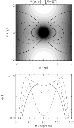
Figure 1: A contour map of the dimensionless effective potential over the $y=0$ plane; white regions corresponds to $\Psi>-0.6$, black regions to $\Psi<-3$, and the intermediate gray levels are spaced in increments $\Delta\Psi=0.15$. Drawn over the map are four selected field lines for a magnetic dipole aligned with the rotation axis; these lines have summit radii $\gamma=\sqrt[3]{2/3}$ (solid), $\sqrt{2}$ (dashed), 2 (dotted) and 4 (dot-dashed), and are oriented at azimuthal angles $\phi=0\degr$ (right) and $\phi=180\degr$ (left). Shown beneath is the dimensionless potential along each of the $\phi=0\degr$ lines, plotted as a function of $\theta$; note that the scale of the ordinate is logarithmic.

In the foregoing discussion, we argue that circumstellar plasma accumulates on the surfaces defined by minima of the field line potential. We now consider the geometry of one such accumulation surface in the simplest of all configurations, that of a centred dipole magnetic field aligned with the star’s rotation axis. Defining a Cartesian coordinate system $(x,y,z)$ with origin at the star’s centre and rotation taken along the $z$-axis, Fig. 1 shows an $x$ vs. $z$ contour map of the dimensionless effective potential $\Psi(\mn@boldsymbol{r})$ (see eqn. 14) in the $y=0$ plane. Superimposed over the map are four curves, each following the parametric equation for a dipole field line,

$$\xi=\gamma\,\sin^{2}\theta.$$ (15)

Here, the parameter $\gamma$ specifies the summit radius (in units of $r_{\textrm{K}}$) of the field line; in the present case of Fig. 1, the $\gamma=\sqrt[3]{2/3}$, $\sqrt{2}$, 2 and 4 lines are plotted. The significance of the first value is discussed below. Beneath the contour map, we plot the dimensionless potential

$$\Psi(\theta)=-\frac{1}{\gamma\sin^{2}\theta}-\frac{1}{2}\gamma^{2}\sin^{6}\theta,$$ (16)

this being $\Psi(\mn@boldsymbol{r})$ sampled along the dipole trajectory (15), for each of the four field lines. For simplicity, we chose the colatitude $\theta$ as the independent variable in the above expression, rather than the usual field line coordinate $s$. However, noting that the two are related via the differential equation

$$\frac{\mathrm{d}s}{\mathrm{d}\theta}=r_{\textrm{K}}\,\gamma\,\sin\theta\sqrt{1+3\cos^{2}\theta},$$ (17)

it is clear that, everywhere away from the poles, $s$ varies monotonically with $\theta$.

Inspecting the $\Psi(\theta)$ data for the three outer field lines ($\gamma=\sqrt{2},2,4$) shown in Fig. 1, minima can be seen at the stellar equator ($\theta=90\degr$). Since the aligned dipole configuration is symmetric about the $z$ axis, we can conclude that the accumulation surface takes the form of an equatorial disk, with its normal pointing along the rotation axis. However, because a potential minimum does not occur along the innermost field line, it is evident that this disk does not extend to the origin, but instead must terminate at some finite radius. To determine this inner truncation radius, we observe that

$$\Psi^{\prime\prime} =\left(\frac{\mathrm{d}\theta}{\mathrm{d}s}\right)^{2}\frac{\mathrm{d}^{2}\Psi}{\mathrm{d}\theta^{2}}+\frac{\mathrm{d}\theta}{\mathrm{d}s}\frac{\mathrm{d}^{2}\theta}{\mathrm{d}s^{2}}\frac{\mathrm{d}\Psi}{\mathrm{d}\theta}$$ (18)

$$=\frac{1}{r_{\textrm{K}}^{2}}\left(-\frac{2}{\xi^{3}}+3\right)$$

for $\theta=90\degr$, where in the second line we make use of the identity $\xi=\gamma$ within the equatorial plane (cf. eqn. 15). We recall that $\Psi^{\prime\prime}$ must be positive in order for an extremum ($\Psi^{\prime}=0$) to constitute part of an accumulation surface; accordingly, the inner truncation radius is given by

$${\xi}_{\rm i}=\sqrt[3]{2/3}\approx 0.87$$ (19)

at which $\Psi^{\prime\prime}$ changes from being positive ($\xi>{\xi}_{\rm i}$) to negative ($\xi<{\xi}_{\rm i}$).

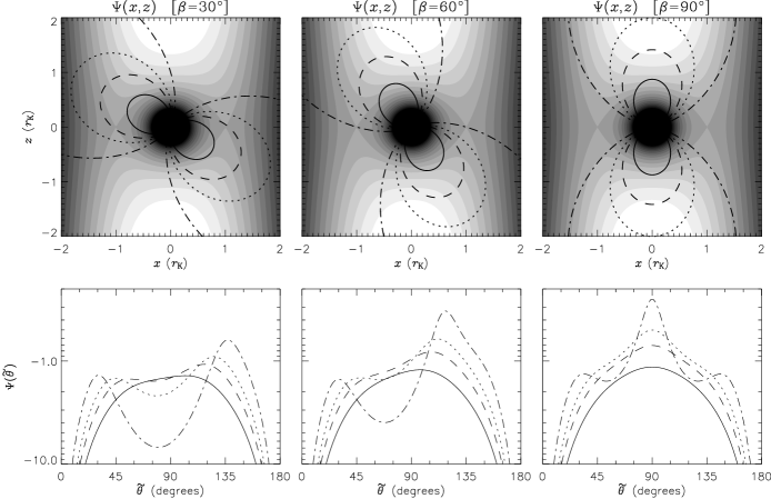
Figure 2: As with Fig. 1, except that a tilted dipole field is assumed, at angles $\beta=30\degr$, $60\degr$ and $90\degr$ to the rotation axis.

The reason for our choice of $\gamma=\sqrt[3]{2/3}={\xi}_{\rm i}$ for the innermost field line in Fig. 1 should now become apparent: it ensures that this particular line exactly intersects the inner edge of the accumulation disk at $\xi={\xi}_{\rm i}$. Plasma at the summit of this line is therefore in neutral equilibrium, whereby small displacements away from the equator produce no net force (to first order in the displacement) along the field line, either away from the equilibrium point or toward it. This is evident in the lower panel of Fig. 1 from the flatness of this field line’s dimensionless potential at $\theta=90\degr$.

Throughout the region in the equatorial plane between the truncation radius $\xi={\xi}_{\rm i}$ and the Kepler co-rotation radius $\xi=1$, magnetic tension supports accumulated material against the net inward pull caused by gravity exceeding the centrifugal force. Beyond this region, when $\xi>1$, the centrifugal force surpasses gravity, and the effect of magnetic tension then becomes to hold material down against the net outward pull.

Clearly, the interplay between gravitational and centrifugal forces has a different significance in the RRM case than it does for a Keplerian disk; in the latter, material at each radius orbits the star at a velocity whereby both forces are in exact balance. Such complete force balance is not required in an RRM, inasmuch that magnetic tension can absorb any net resultant force perpendicular to field lines (Preuss et al., 2004). Only the tangential components of the forces are required to be in balance, so as to produce an equilibrium that is stable against small displacements along field lines – a point recognized in the original treatment by Michel & Sturrock (1974), although these authors employed a more-geometrical approach to arrive at the same conclusion.

2.3 The tilted dipole configuration

Up until now, we have dealt with the trivial case of a dipole field aligned with the rotation axis. However, there is nothing that restricts us to such simple systems; as Nakajima (1985) first demonstrated, the rigid-field approach we have presented can be applied to arbitrary magnetic configurations, so long as the effective potential along each field line can be computed and minimized.

In the present section we now consider the oblique rotator configuration, where a dipole is inclined at an angle $\beta$ to the rotation axis. For such a geometry, eqn. (11) still describes the effective potential in the co-rotating frame, but the field lines of the tilted dipole now follow the parametric equation

$$\xi=\gamma\sin^{2}\tilde{\theta},$$ (20)

where $\tilde{\theta}$ is the colatitude coordinate in the frame of reference aligned with the magnetic axis. To relate this magnetic reference frame back to the rotational one, we adopt the convention that the former is obtained from the latter by rotating by an angle $\beta$ about the Cartesian $y$ axis. With this convention, colatitudes in the two reference frames are related to one another via

$$\sin^{2}\theta=\sin^{2}\tilde{\theta}\,\sin^{2}\tilde{\phi}+\mbox{}\\ \left(\sin\beta\,\cos\tilde{\theta}+\cos\beta\,\sin\tilde{\theta}\,\cos\tilde{\phi}\right)^{2},$$ (21)

were $\tilde{\phi}$ denotes the azimuthal coordinate in the magnetic frame.

The latter expression may be used to eliminate the $\sin^{2}\theta$ term from eqn. (14), allowing us to express the dimensionless effective potential along each field line as

$$\Psi(\tilde{\theta})=-\frac{1}{\gamma\sin^{2}\tilde{\theta}}-\frac{1}{2}\gamma^{2}\sin^{4}\tilde{\theta}\left[\sin^{2}\tilde{\theta}\,\sin^{2}\tilde{\phi}+\mbox{}\right.\\ \left.\left(\sin\beta\,\cos\tilde{\theta}+\cos\beta\,\sin\tilde{\theta}\,\cos\tilde{\phi}\right)^{2}\right];$$ (22)

here, we have also used eqn. (20) to eliminate $\xi$. It is straightforward to derive an expression for the derivative $\Psi^{\prime}$ of this field line potential; however, in contrast to the aligned dipole configuration, the equation $\Psi^{\prime}=0$ for the extrema of this potential no longer admits algebraic solutions. But in the $x$–$z$ plane that contains both the magnetic and rotation axes, we can still illustrate these minima using the same graphical approach as in Sec. 2.2.

Figure 2 shows similar effective potential plots to Fig. 1, but for dipole field configurations tilted at angles $\beta=30\degr$, $60\degr$ and $90\degr$ to the rotation axis. Focusing initially on the first two cases, we note that a single potential minimum occurs along the outer three field lines when $\beta=30\degr$, and along the outer two for $\beta=60\degr$. In each case, the minima are situated at approximately the same colatitude, which falls somewhere between the magnetic and rotational equators: $\tilde{\theta}\approx 80\degr$ for $\beta=30\degr$, and $\tilde{\theta}\approx 70\degr$ for $\beta=60\degr$. This bisection of the equators arises because of competition between the two misaligned symmetry axes, magnetic vs. rotational.

Looking now at the $\beta=90\degr$ case, we can see that two minima – albeit shallow ones – occur in the potential along the outermost field line, at equal distances above ($\tilde{\theta}\approx 55\degr$) and below ($\tilde{\theta}\approx 125\degr$) the magnetic equator. This shows that the accumulation surfaces of tilted configurations can be significantly more complex than the simple disk found for the aligned dipole; indeed, as we demonstrate in the following section, there is no guarantee even that the surfaces are made from a single contiguous sheet. Nakajima (1985) overlooked such situations, and it was not until the study by Preuss et al. (2004) that this possibility became known.

To conclude this section, we draw attention to a limitation of the graphical approach we have used to illustrate the accumulation surfaces: although these surfaces are inherently three dimensional, our approach is restricted to plotting the effective potential and magnetic field lines over a two dimensional slice through the system. This is not a problem for the aligned dipole shown in Fig. 1, since rotational symmetry ensures that all slices containing the polar axis are identical. However, this symmetry is absent from the tilted field configurations plotted in Fig. 2, meaning that the figure cannot indicate the nature of the accumulation surfaces outside of the $x$–$z$ plane that contains the misaligned rotation and magnetic axes.

3 Accumulation Surfaces

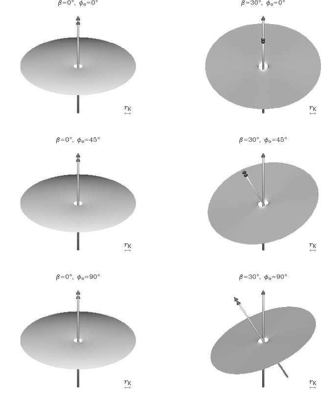
Figure 3: Accumulation surfaces for aligned ($\beta=0\degr$; left-hand column) and tilted ($\beta=30\degr$; right-hand column) dipole magnetic fields; the surfaces are viewed at an inclination $i=60\degr$ to the rotation axis, and from azimuths (top-to-bottom) $\phi_{\rm o}=0\degr$, $45\degr$ and $90\degr$. In each plot, the rotation and magnetic axes are shown as single- and double-headed arrows, respectively; to indicate the scale of the plots, a bar with a length of one Kepler radius ($r_{\textrm{K}}$) is shown in the bottom right-hand corner of each.

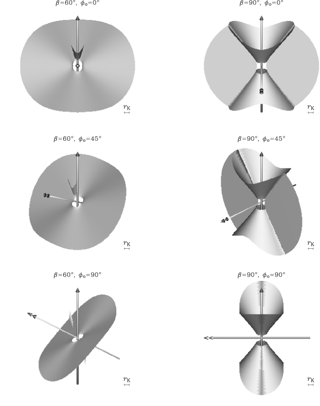
Figure 4: continued

As before, except that the tilted configurations for $\beta=60\degr$ (left-hand column) and $\beta=90\degr$ (right-hand column) are shown.

To overcome these limitations of two-dimensional plots, let us now use perspective images to show the full three-dimensional form of the accumulation surfaces. For the same aligned and tilted dipole magnetic field configurations introduced above, Fig. 3 illustrates these as surfaces illuminated by an artificial parallel light source from the observation point. The vertical, single-headed arrows denote the rotation axis, while the double-headed arrows shown in projection at various orientations represent the magnetic axis. For each of the four values of the tilt angle $\beta=\{0\degr,30\degr,60\degr,90\degr\}$, the accumulation surface is shown from three different observation points, situated at the same inclination $i=60\degr$ to the rotation axis, but having differing azimuthal angles $\phi_{\rm o}=0\degr$, $45\degr$ and $90\degr$. Although the full surfaces formally extend to arbitrarily large radii, for the illustration the outer edge is truncated by omitting regions threaded by field lines with summit radii greater than $\gamma=12$.

For the aligned field ($\beta=0\degr$) case, the accumulation surface is a simple disk lying in the plane of the rotational and magnetic equators, and so appears identical from all azimuths. The hole at the centre reflects the lack of potential minima inside the inner truncation radius ${\xi}_{\rm i}$ (Sec. 2.2). For the $\beta=30\degr$ case the surface is titled, with a mean normal vector between the two symmetry axes, in a direction consistent with the $\tilde{\theta}\approx 80\degr$ angle found in Sec. 2.3. Although not obvious in Fig. 3, the surface is not strictly planar, but has a slight warp.

For the greater tilt of the $\beta=60\degr$ configuration, this warping becomes more apparent. While still shaped approximately like a disk, the regions nearest the intersection with the plane formed by the two axes are warped away from the rotation axis. Physically, this arises because the centrifugal force vanishes along the rotation axis; this force being crucial to forming the potential minima that make up the accumulation surface, it follows that there is a ‘zone of avoidance’ around the rotation axis, inside of which the surface cannot exist. An additional, remarkable feature of the $\beta=60\degr$ case is the appearance of a pair of secondary accumulation surfaces, situated in each hemisphere between the magnetic and rotation axes. These secondary surfaces, which we term leaves, are a consequence of the appearance of an additional minimum in the effective potential along a particular bundle of magnetic field lines.

From the analysis in Sec. 2.3, it might appear that such two-minima scenarios are restricted to the perpendicular ($\beta=90\degr$) configuration; however, the appearance of the leaves in this intermediate-tilt case proves otherwise. In fact, as Preuss et al. (2004) have demonstrated, leaves occur in all configurations other than the aligned field one, but are situated at larger and larger radii as $\beta$ decreases toward zero. In the present case with $\beta=60\degr$, the leaves are threaded by magnetic field lines for which $\gamma\gtrsim 10$; this explains why the middle panel of Fig. 2, which plots field lines up to $\gamma=4$, does not exhibit the second potential minimum associated with the appearance of a leaf.

Turning finally to the perpendicular field ($\beta=90\degr$) configuration, we see the ultimate product of the disk warping and leaf formation. The accumulation surface now takes the form of a partial disk lying in the magnetic equator, intersected by an opposing pair of truncated cones aligned with the rotation axis. These cones have an opening half-angle of $\tan^{-1}2^{-1/2}\approx 35.3\degr$ at asymptotically-large radii, a value that can be derived by setting the first derivative of $\Psi(\tilde{\theta})$ (cf. eqn. 22) to zero, and then solving for $\tilde{\theta}$ as $\gamma\rightarrow\infty$ (see also Preuss et al., 2004). To understand the unusual geometry of the perpendicular configuration, note that if $\beta$ were to depart slightly from $90\degr$, then the half of each cone that lies between the two axes would split off from the main accumulation surface, and take the form of a leaf. Therefore, we can recognize the cones as being formed from a merger between the warped disk and the leaves.

The geometrical complexity of accumulation surfaces, even in the relatively-simple case of a tilted dipole, was unknown to Nakajima (1985); he had to rely on simple particle-based maps for visualization (see his figs. 2 & 3), and was unaware of the possibility of leaves or of the truncated-cone configuration occurring at $\beta=90\degr$. Only in recent years have computers become sufficiently powerful that the visualization of the surfaces is a relatively straightforward procedure. However, there still remains the question of how closely a physical system would resemble an accumulation surface. The answer depends on the nature and distribution of the matter that populates the surfaces and renders them visible or detectable. While the accumulation surfaces presented in this section, and by Preuss et al. (2004), furnish a geometrical picture of where circumstellar material can accumulate, they provide no indication of how much material does accumulate, nor of its physical conditions – density, temperature, opacity, emissivity, etc.. We address these issues in the following sections, where we derive the distribution of circumstellar gas, and then use this to calculate the line emission from an RRM model.

4 Hydrostatic Stratification

The various processes that could fill effective potential wells with material may generally be quite dynamic and variable; but over time, it seems likely that most such material should eventually settle into a nearly steady, static state. Along any given field line that intersects with one or more of the potential minima that define accumulation surfaces, the relative distribution of material density $\rho$ is then set by the requirement of hydrostatic stratification within the field line potential,

$$\frac{\mathrm{d}p}{\mathrm{d}s}=-\rho\frac{\mathrm{d}\Phi}{\mathrm{d}s}\,,$$ (23)

where the gas pressure is given by the ideal gas law,

$$p=\frac{\rho kT}{\mu}\,.$$ (24)

Taking for simplicity the temperature $T$ and mean molecular weight $\mu$ to be constant, we can solve for the density distribution along the field line as

$$\rho(s)=\rho_{m}\,e^{-\mu[\Phi(s)-\Phi_{\rm m}]/kT}\,,$$ (25)

where $\rho_{\rm m}\equiv\rho(s_{\rm m})$ and $\Phi_{\rm m}\equiv\Phi(s_{\rm m})$, with $s_{\rm m}$ the field line coordinate at the potential minimum. In our application to magnetic hot stars, we assume radiative equilibrium should set the circumstellar temperature to be near the stellar effective temperature. This implies a thermal energy per unit mass $kT/\mu$ that is much smaller than the variation in the corresponding potential energy $\Phi$, which by eqn. (13) is typically comparable or greater than the gravitational binding energy at the Kepler radius. By eqn. (25), we thus expect that most of the material should be confined to a relative narrow layer near the potential minimum at $s=s_{\rm m}$.

A Taylor series expansion of the potential about this minimum gives

$$\Phi(s)=\Phi_{\rm m}+\frac{(s-s_{\rm m})^{2}}{2}\Phi_{\rm m}^{\prime\prime}+\ldots,$$ (26)

where we have used the fact that, by definition, $\Phi_{\rm m}^{\prime}=0$. Accordingly, in the neighborhood of the minimum, the density distribution (25) may be well approximated by

$$\rho(s)\approx\rho_{\rm m}\,e^{-(s-s_{\rm m})^{2}/0pt^{2}},$$ (27)

where the RRM scale height is

$$0pt=\sqrt{\frac{2kT/\mu}{\Phi_{\rm m}^{\prime\prime}}}=\sqrt{\frac{2kT/\mu}{GM_{\ast}/r_{\textrm{K}}}}\,\sqrt{\frac{1}{\Psi_{\rm m}^{\prime\prime}}}.$$ (28)

In the latter equality, the first square root is of the ratio between the thermal energy and the gravitational binding energy at the Kepler radius, while the second root gives the curvature length of the effective potential. Overall, we thus see that the effect of a finite gas pressure is to support material in a nearly Gaussian stratification on either side of an accumulation surface.

A similar Gaussian stratification is found in models for Keplerian disks; however, the scale height in that case grows as the three-halves power of the distance from disk centre (e.g., Hummel & Hanuschik, 1997), leading to a disk that flares outward with increasing radius. In contrast, the RRM scale height approaches a constant value far from the origin; for example, in the case of the aligned dipole configuration, eqn. (18) gives $\Psi_{\rm m}^{\prime\prime}=3/r_{\textrm{K}}^{2}$ when $\xi^{3}\gg 1$, yielding the asymptotic scale height

$$0pt\rightarrow r_{\textrm{K}}\sqrt{\frac{2kT/\mu}{3GM_{\ast}/r_{\textrm{K}}}}\qquad(r\gg r_{\textrm{K}})\,$$ (29)

(compare with eqn. 5 of Nakajima, 1985). Since the ratio of thermal energy to gravitational binding energy is typically very small, we thus see that the disk is indeed geometrically thin, with a scale height 0pt that is much smaller than the characteristic Kepler radius $r_{\textrm{K}}$.

A convenient way to characterize the properties of such a thin accumulation layer is in terms of its surface density. For field line with a projection cosine $\mu_{\rm m}$ to the surface normal, the associated local surface density $\sigma_{\rm m}$ can be obtained by integration of eqn. (27) over the Gaussian hydrostatic stratification,

$$\sigma_{\rm m}\approx\sqrt{\pi}\rho_{\rm m}\mu_{\rm m}0pt\,.$$ (30)

For the application here to magnetic hot stars, we next develop a specific model for the global distribution of this surface density as being proportional to the rate of material build-up by the loading from the star’s radiatively driven wind.

5 Mass Loading of Accumulation Surfaces

5.1 The Accumulation Rate for Surface Density

The high luminosity of hot stars is understood to give rise to a radiatively driven stellar wind; in a magnetic hot star, this wind provides a key mechanism to load mass into the effective gravito-centrifugal potential wells around the accumulation surfaces.

For a radiatively driven wind in the presence of a magnetic field, Owocki & ud-Doula (2004) derive an expression for the mass flux density at the stellar surface, in terms of the spherical mass loss rate $\dot{M}$ predicted by the standard CAK wind model (Castor et al., 1975). For a dipole flux-tube bundle intersecting the stellar surface $r=R_{\ast}$ with a projection cosine $\mu_{\rm\ast}$, and having a cross-sectional area $\mathrm{d}A_{\rm\ast}$, the rate of mass increase is

$$\dot{m}\ =\frac{2\mu_{\rm\ast}\dot{M}}{4\pi R_{\ast}^{2}}\,\mathrm{d}A_{\rm\ast}\,,$$ (31)

where the factor 2 accounts for the mass injection from two distinct footpoints.

In a highly supersonic stellar wind, the collision of material from opposite footpoints leads to strong shocks that heat the plasma initially to temperatures of millions of degrees; this dogma, advanced by Babel & Montmerle (1997a, b) in their MCWS paradigm, has been amply confirmed both by MHD modeling (e.g., ud-Doula & Owocki, 2002), and by analysis of the observed X-ray emission from the superheated post-shock plasma (e.g., Gagné et al., 2004). Eventually, the plasma cools radiatively back to temperatures near the stellar effective temperature of a few times $10^{4}\,\textrm{K}$. As discussed already in Sec. 4, at such temperatures material trapped within the effective potential well will quickly settle into a relatively narrow hydrostatic stratification centred on the potential minima.

For the moment, let us consider the relatively simple, common case that there is a single minimum at field line coordinate $s_{\rm m}$, at which point the flux tube has area $\mathrm{d}A_{\rm m}$ and intersection cosine $\mu_{\rm m}$ with the accumulation surface normal. Then the associated rate of increase in surface density $\sigma_{\rm m}$ can be written

$$\dot{\sigma}_{\rm m}=\dot{m}\mu_{\rm m}/\mathrm{d}A_{\rm m}=\mu_{\rm m}\,\mu_{\rm\ast}\,\frac{\dot{M}}{2\pi R_{\ast}^{2}}\,\frac{\mathrm{d}A_{\rm\ast}}{\mathrm{d}A_{\rm m}}\,.$$ (32)

From the conservation of magnetic flux, $\nabla\cdot\mn@boldsymbol{B}=0$, we have

$$\mathrm{d}A_{\rm\ast}B_{\ast}=\mathrm{d}A_{\rm m}B_{\rm m}\,,$$ (33)

which when applied to eqn. (32) gives

$$\dot{\sigma}_{\rm m}=\mu_{\rm\ast}\,\mu_{\rm m}\,\frac{\dot{M}}{2\pi R_{\ast}^{2}}\,\frac{B_{\rm m}}{B_{\ast}}\,.$$ (34)

For a dipole field, this declines with radius $r$ as $\dot{\sigma}_{\rm m}\propto B\propto r^{-3}$.

5.2 The Time Evolution of the Volume Density

The above merely gives the rate at which surface density increases in the accumulation surface. In the idealized limit that the field is arbitrarily strong, the actual surface density could thus increase without bound. In reality, for any large but finite field, the finite magnetic tension could only contain a finite mass of material. As analyzed in the Appendix, above some breakout density the net centrifugal and gravitational force should overwhelm the tension, leading to centrifugal ejection that effectively empties the accumulation surface.

This view suggests a simple model in which the local surface density builds linearly with the time $t$ since the last evacuation, $\sigma_{\rm m}=\dot{\sigma}_{\rm m}t$. Applying such a model to eqns (30) and (34), we can eliminate the normalizing term $\rho_{\rm m}$ from the equation (25) for the volume density, to find the time evolution of this density as

$$\rho(s,t)\approx\frac{\dot{M}t\,\mu_{\rm\ast}}{2\pi^{3/2}R_{\ast}^{2}\,0pt}\,\frac{B_{\rm m}}{B_{\ast}}\,e^{-\mu[\Phi(s)-\Phi_{\rm m}]/kT}\,.$$ (35)

For field lines that exhibit two potential minima, we divide the latter expression by the factor

$$f=1+\frac{h^{\dagger}_{\rm m}}{0pt}\,\frac{B_{\rm m}}{B^{\dagger}_{\rm m}}\,e^{\mu[\Phi_{\rm m}-\Phi^{\dagger}_{\rm m}]/kT},$$ (36)

where $h^{\dagger}_{\rm m}$, $B^{\dagger}_{\rm m}$ and $\Phi^{\dagger}_{\rm m}$ are the scale height, field strength and potential evaluated at the secondary minimum with field line coordinate $s^{\dagger}_{\rm m}$. This factor accounts for the partitioning of plasma between the two minima, assuming a free exchange of material leads to a common hydrostatic stratification.

We emphasize that eqn. (35) applies only to field lines that intersect one or more accumulation surfaces, with one or more potential minima. For all other field lines we set the density to zero, reflecting the notion that there can be no stable accumulation of material over time. Moreover, even for field lines intersecting a surface, we only apply eqn. (35) up to the bracketing maxima in the potential. Beyond these maxima, the decreasing potential suggests an exponentially growing density, contrary to the true physical picture of no accumulation. We resolve this difficulty by setting the density $\rho$ to zero in the regions beyond the potential maxima. This approach creates discontinuities in the densities at the maxima themselves, but in most cases ones so small that they are unlikely to be of much significance for the overall model.

6 Circumstellar Emission

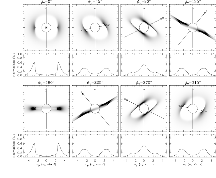
Figure 5: Maps of the emission from the $\beta=60\degr$ RRM model (see text), for eight different values of the observer azimuth $\phi_{\rm o}$; darker shading indicates greater intensity. In each map, the rotation and magnetic axes are shown as a single- and double-headed arrows, while the outline of the central star (whose contributions toward the emission are neglected) is shown by a circle. Beneath each map, we plot the corresponding emission spectrum as a function of the projected velocity $v_{\rm p}$, the latter being measured in units of the projected equatorial rotation velocity $v_{\rm e}\sin i$ of the star.

Let us now apply the expression (35) for the density distribution toward calculating the circumstellar line emission from a tilted-dipole RRM configuration. As a typical example case, we adopt a tilt angle $\beta=60\degr$, and set the stellar angular velocity $\Omega$ to 50 percent of the critical rate,

$$\Omega_{\rm c}\equiv\sqrt{\frac{8GM_{\ast}}{27R_{\ast}^{3}}}\,,$$ (37)

at which the surface centrifugal force at the equator would balance gravity; this rotation rate corresponds to a dimensionless stellar radius $\xi_{\ast}\equiv R_{\ast}/r_{\textrm{K}}=0.42$. Our choice of parameters is loosely guided by the rotation rate and magnetic tilt inferred from the Groote & Hunger (1997) model for the surface of $\sigma$ Ori E; however, we make no attempt at fine tuning, since we are more concerned here with demonstrating the capabilities of the RRM model, than with obtaining an accurate picture of this particular helium-strong star.

To specify the temperature $T$ and mean molecular weight $\mu$ in the model, we introduce the dimensionless quantity

$$\varepsilon_{\ast}\equiv\frac{kTR_{\ast}}{\mu GM_{\ast}},$$ (38)

which characterizes the ratio of thermal to gravitational binding energy at the stellar surface. In the photospheres of early-type stars, this ratio is of the order $\sim 10^{-3}$. Following again the scenario that the circumstellar environment remains at a temperature close to photospheric (cf. Sec. 4), we therefore set $\varepsilon_{\ast}=10^{-3}$ throughout.

We now make the assumption that the plasma volume emissivity $j_{\lambda}$, at a wavelength $\lambda$, may be characterized by the relation

$$j_{\lambda}=j_{0}\,\rho^{2}\,\delta(\lambda-\lambda_{0});$$ (39)

here, $j_{0}$ and $\lambda_{0}$ are constants, and $\delta(\ldots)$ is the Dirac delta function. This expression is intended to mirror the process of monochromatic line emission at a rest-frame wavelength $\lambda_{0}$, arising from the density-squared radiative recombination of ionized hydrogen. Integrating the emissivity along a given ray passing through the magnetosphere, the observed surface intensity of the emission is given by

$$\mathcal{I}_{\lambda}=j_{0}\,\int_{0}^{\infty}\rho^{2}(z_{\rm o})\,\delta(\lambda-\lambda_{0}[1+v_{\rm p}(z_{\rm o})/c])\,\mathrm{d}z_{\rm o},$$ (40)

where $z_{\rm o}$ is the distance along the ray from the observer, $v_{\rm p}$ is the projection of the local plasma velocity onto the ray, and $c$ is the speed of light. For rays intersecting the star, this integral must be truncated at the stellar surface, to account for the occultation of radiation incident from the star’s far side. Note that this simple expression does not include the emission of radiation by the star itself; therefore, it should be taken to represent the notional circumstellar component of the net radiation from the system, with the understanding that the corresponding photospheric component has been subtracted away. Of course, such an interpretation is in itself an approximation, since our emission model does not account for episodes when circumstellar plasma transits the disk and absorbs stellar radiation over the range $-v_{\rm e}\sin i<v_{\rm p}<v_{\rm e}\sin i$; however, at the level of the present investigation, this approximation is entirely sufficient.

Because the magnetospheric plasma co-rotates rigidly with the star, $v_{\rm p}$ may be expressed as

$$v_{\rm p}(z_{\rm o})=\Delta\,v_{\rm e}\sin i,$$ (41)

where the impact parameter $\Delta$ is the perpendicular distance, in units of $R_{\ast}$, between the ray and the rotation axis, and $v_{\rm e}$ is the equatorial rotation velocity of the star. These quantities, and therefore $v_{\rm p}$ too, are independent of $z_{\rm o}$; hence, the intensity may be written in the form

$$\mathcal{I}_{\lambda}=j_{0}\,\delta(\lambda-\lambda_{0}[1+\Delta\,v_{\rm e}\sin i/c])\,\int_{0}^{\infty}\rho^{2}(z_{\rm o})\,\mathrm{d}z_{\rm o}.$$ (42)

From this latter expression, it can be seen that all plasma having the same $\Delta$ – that is, situated on a plane parallel to the rotation axis – will radiate monochromatically at the same wavelength.

Applying eqn. (42) to the known density distribution of the $\beta=60\degr$ RRM configuration, Fig. 5 shows maps of the wavelength-integrated emission intensity

$$\mathcal{I}\equiv\int_{0}^{\infty}\mathcal{I}_{\lambda}\,\mathrm{d}\lambda,$$ (43)

extending out to 5 $R_{\ast}$ in directions parallel and perpendicular to the projected rotation axis. The observer is situated at the same inclination $i=60\degr$ that we adopt in Sec. 3, and at eight differing values of the azimuth $\phi_{\rm o}$, separated by uniform increments of $45\degr$. Beneath each map we show the corresponding spectrum, in which the spatially-integrated emission is plotted as a function of the projected velocity $v_{\rm p}$. Since we are interested more in the distribution of emission than its absolute value, Fig. 5 adopts an arbitrary (although consistent) normalization for the intensities in both the maps and the spectra.

In Section 3, we demonstrate that the accumulation surface for a $\beta=60\degr$ tilted dipole takes the form of a warped disk. The emission maps in Fig. 5 reveal that the distribution of material across this disk is decidedly non-uniform. Specifically, the distribution is dominated by two clouds, located near the inner edge of the disk at the intersection between the rotational and magnetic equators. Seen from an inertial frame, these clouds appear to rotate synchronously with the star; furthermore, their characteristic twin-peaked emission spectrum displays temporal variations in the form of a double S-wave.

These findings exhibit an encouraging degree of agreement with the inferred behaviour of $\sigma$ Ori E. As discussed in the introduction, observations of this star indicate that circumstellar plasma is concentrated at the intersection between rotational and magnetic equators (Groote & Hunger, 1982; Bolton et al., 1987; Short & Bolton, 1994). Without the need for any special tuning, beyond the requirement that the tilt angle $\beta$ be moderate, the RRM model naturally reproduces such a distribution. It also accounts for the Balmer line emission from the star, which – when the measured longitudinal field is strongest, corresponding to $\phi_{\rm o}=0\degr$ and $\phi_{\rm o}=180\degr$ in Fig. 5 – is observed to exhibit strong peaks situated at $v_{\rm p}\approx\pm 3v_{\rm e}\sin i$ (Groote, personal communication).

7 Discussion

As we discuss in Sec. 1, there have been a number of previous studies that have made use of the rigid-field approach (cf. Sec. 2) to determining the regions where circumstellar material can accumulate (Sec. 3). The present paper builds on these studies, by presenting a physically-grounded RRM model for the steady accumulation of wind plasma in the circumstellar environment (Secs. 4 & 5), that is able to make specific predictions regarding the observables associated with this plasma (Sec. 6).

Our treatment of the mass loading of accumulation surfaces differs markedly from the approach advanced by Nakajima (1985), who fixed the plasma density at each point by requiring equal magnetic and kinetic energy densities (see his eqn. 13); such a choice is guided by the notion that when the density is high enough for the kinetic energy due to rotation to dominate the magnetic energy, the field lines break open, and any subsequently-added plasma leaks away from the system. By contrast, our approach to deriving the plasma distribution focuses on the mass accumulation rather than on leakage (cf. Sec. 5). While Nakajima (1985) treats the mass leakage as a gradual, quasi-steady process, we view it more as an episodic evacuation caused by magnetic breakout (see Appendix), which effectively resets the mass accumulation.

In actual systems the mass distribution may reflect a combination of both perspectives, and there are even other alternative frameworks for treating the problem (see, e.g., Michel & Sturrock, 1974; Havnes & Goertz, 1984). However, one particularly favourable aspect of the present model is that it can naturally reproduce the plasma concentrations at the intersection of rotational and magnetic equators, as is inferred from observations of $\sigma$ Ori E. To obtain a similar result, Nakajima (1985) had to make the ad hoc assumption that some process of diffusion, across magnetic field lines, leads to the redistribution of plasma into the desired configuration.

We turn now to a brief discussion of the recent paper by Preuss et al. (2004), which was published during the final stages of preparation of the present work. These authors found the same accumulation surfaces as we present in Sec. 3, but using the alternative formulation based around consideration of the loci where all forces tangential to field lines vanish. They were the first to discover the possibility of leaves and the truncated cones occurring at $\beta=90\degr$, and even explored the case of tilted dipoles offset from the origin. However, Preuss et al. (2004) stopped short of considering the mass loading of the accumulation surfaces, and instead focused on their geometrical form. As such, their study does not make the kind of specific predictions for observable emission line variations that we provide in Sec. 6.

Another relevant comparison here is to the Magnetically Torqued Disk (MTD) model proposed by Cassinelli et al. (2002) to explain the circumstellar emission of Be stars. Building upon insights from one-dimensional equatorial plane models of magnetically torqued stellar winds (Weber & Davis, 1967; Belcher & MacGregor, 1976), this analysis centres on an assumed empirical scaling of the azimuthal velocity, which initially increases as a rigid-body law out to some peak, and then declines asymptotically with angular momentum conservation. When this peak occurs above the Kepler radius, the model envisions that the associated torquing of the wind outflow can lead to formation of a ‘quasi-Keplerian’ disk. But recent dynamical simulations (Owocki & ud-Doula, 2003) indicate that fields marginally strong enough to spin wind material beyond Keplerian rotation tend instead to lead to centrifugal mass ejection rather than a Keplerian disk.

For much stronger fields, the region of rigid rotation becomes more extended, and the MTD scenario can be viewed as becoming similar to the field-aligned rotation case ($\beta=0$) of the RRM model developed here. Although the disk rotation is rigid-body rather than Keplerian, the tendency for the bulk of the material to build up in the region near the Kepler radius means that the resulting line emission should develop a doubled-peaked profile that might be quite difficult to distinguish from what is expected from a Keplerian disk. Note, however, that such rigid-body disks seem unlikely to produce the long-term (years to decade) violet/red (V/R) variations often observed in Be-star emission lines (Telting et al., 1994); such variations seem instead likely to be the result of long-term precession of elliptical orbits within a Keplerian disk (Savonije & Heemskerk, 1993). As such, we do not believe that the RRM model is likely to be of general relevance to explaining Be star emission. However, as noted above, it does seem quite well-suited to explaining the rotationally modulated emission of Bp stars like $\sigma$ Ori E.

On a concluding note, we draw attention to the fact that X-ray flaring has been detected in $\sigma$ Ori E by ROSAT (Groote & Schmitt, 2004), and subsequently by XMM-Newton (Sanz-Forcada et al., 2004). Mullan (2004) has argued that the flares originate from the B2 star itself, rather than from an unseen low-mass companion. If this is indeed the case, then we suggest a likely mechanism for the flare generation is thermal heating arising from magnetic reconnection. As we discuss in the Appendix, we expect the outer parts of the accumulation surface to undergo relatively frequent breakout events, during which stressed magnetic field lines will reconnect and release significant quantities of energy. We intend to explore this hypothesis further in a future paper (and see also ud-Doula et al., 2004).

8 Summary

We have presented a new Rigidly Rotating Magnetosphere model for the circumstellar plasma distributed around magnetic early-type stars. By assuming that field lines remain completely rigid, and co-rotate with the star, we are able to find regions in the circumstellar environment where plasma can accumulate under hydrostatic equilibrium; in the general case of a tilted dipole field, these regions take the form of a geometrically-thin, warped disk, whose mean surface normal lies between the misaligned magnetic and rotation axes. When coupled with a quantitative description of the accumulation process, our treatment allows us to evaluate the density throughout the circumstellar environment, and thereby calculate observables such as emission-line spectra.

This RRM model shows promise; even without a fine tuning of parameters, it reproduces the principal features of $\sigma$ Ori E, the archetype of the variable-emission helium-strong stars. In a forthcoming paper, we will investigate the extent to which the model can reproduce the more detailed aspects of this star – in particular, the strength of the emission lines, as well as their shape, and the eclipse-line variations seen in photometric indices. We also plan to examine whether the model can be applied to other magnetic early-type stars.

Appendix A Breakout of Accumulated Material

A.1 Breakout Time

In deriving the form of the accumulation surfaces, we have assumed an arbitrarily strong, rigid field. But in practice the finite magnitude of any stellar magnetic field means that there is a limit to the mass that can be contained against the centrifugal force; when the density gets too high, the material should break out from the field containment. Just prior to such an episode, the over-stressed magnetic field becomes distorted from its equilibrium configuration, sagging radially outward as it passes through the dense material in accumulation surfaces. Under these circumstances, the inward force arising from the tension in the distorted field lines barely balances the net outward gravito-centrifugal force; therefore, we can construct an approximate condition for the occurrence of breakout by equating these two forces. Focusing our analysis in this appendix on the simple case of an aligned dipole field ($\beta=0\degr$), the breakout condition may be expressed as

$$\rho_{\rm b}\left[\Omega^{2}r-\frac{GM_{\ast}}{r^{2}}\right]\approx\frac{B^{2}}{4\pi 0pt},$$ (44)

where $\rho_{\rm b}$ represents a breakout value for the peak density at radius $r$ within the equatorial plane, and the scale height 0pt appears as the typical curvature radius of the distorted magnetic field lines, whose tension $B^{2}/4\pi$ generates the balancing inward force. In analogy with eqn. (30) we can define an associated breakout surface density $\sigma_{\rm b}\equiv\sqrt{\pi}\rho_{\rm b}0pt$, where we have taken $\mu_{\rm m}=1$ as appropriate to the equatorial plane. Using the Kepler radius $r_{\textrm{K}}$ (eqn. 12) to scale both the local radius ($\xi\equiv r/r_{\textrm{K}}$) and the stellar radius ($\xi_{\ast}\equiv R_{\ast}/r_{\textrm{K}}$), we have for the usual dipole field scaling $B\sim r^{-3}$,

$$\sigma_{\rm b}g_{\ast}\xi_{\ast}^{2}\left[\xi-\frac{1}{\xi^{2}}\right]=\frac{B_{\ast}^{2}\xi_{\ast}^{6}}{4\pi\xi^{6}}\sqrt{\pi}\,,$$ (45)

or, solving for the breakout surface density,

$$\sigma_{\rm b}(\xi)=\frac{B_{\ast}^{2}\xi_{\ast}^{4}}{4\pi g_{\ast}}\,\frac{\sqrt{\pi}}{\xi^{4}(\xi^{3}-1)}.$$ (46)

Scaled in terms of typical parameters for a rotating, magnetic B-star, we find a characteristic surface density for breakout

$$\sigma_{\ast}\equiv\frac{B_{\ast}^{2}\xi_{\ast}^{4}}{4\pi g_{\ast}}\approx 8\,\textrm{g}\,\textrm{cm}^{-2}\,\frac{B_{3}^{2}\xi_{\ast}^{4}}{g_{4}}\,,$$ (47)

where $B_{3}\equiv B/10^{3}\,\textrm{G}$ and $g_{4}\equiv g_{\ast}/10^{4}\,\textrm{cm}\,\textrm{s}^{-2}$.

For comparison, note that for a dipole field the surface density accumulation rate in eqn. (34) has the scaling

$$\dot{\sigma}_{\rm m}(\xi)=\mu_{\rm\ast}\,\frac{\xi_{\ast}^{3}}{\xi^{3}}\,\frac{\dot{M}}{2\pi R_{\ast}^{2}}\,,$$ (48)

where once more we have assumed $\mu_{\rm m}=1$. Then for each scaled radius $\xi$ we can define a characteristic breakout time, $t_{\rm b}(\xi)\equiv\sigma_{\rm b}/\dot{\sigma}_{\rm m}$. Casting the stellar gravity in terms of the surface escape speed and free-fall time, $g_{\ast}=v_{\rm esc}/2t_{\rm ff}$, the ratio of breakout to free-fall time becomes

$$\frac{t_{\rm b}(\xi)}{t_{\rm ff}}=\eta_{\ast}\,\frac{\sqrt{\pi}}{\mu_{\rm\ast}}\,\frac{\xi_{\ast}}{\xi(\xi^{3}-1)}\,.$$ (49)

Here we have collected dimensional quantities in terms of a single, dimensionless magnetic confinement parameter for the accumulation surface,

$$\eta_{\ast}\equiv\frac{B_{\ast}^{2}R_{\ast}^{2}}{\dot{M}v_{\rm esc}}\approx 1.6\times 10^{6}\,\frac{B_{3}^{2}R_{12}^{2}}{\dot{M}_{-10}\,v_{8}}\,,$$ (50)

with the latter equality giving a characteristic value in terms of scaled parameters $R_{12}\equiv R_{\ast}/10^{12}\,\textrm{cm}$, $\dot{M}_{-10}\equiv\dot{M}/10^{-10}\,\textrm{M}_{\odot}\,\textrm{yr}^{-1}$, and $v_{8}\equiv v_{\rm esc}/10^{8}\,\textrm{cm}\,\textrm{s}^{-1}$. Noting that the free fall time $t_{\rm ff}=v_{\rm esc}/2g_{\ast}=10^{4}\,{\rm s}\,(v_{8}/2g_{4})$, the breakout time evaluates to

$$t_{\rm b}(\xi)\approx 250\,\textrm{yr}\,\frac{B_{3}^{2}R_{12}^{2}\xi_{\ast}}{\dot{M}_{-10}\,g_{4}}\,\frac{1}{\xi(\xi^{3}-1)}\,,$$ (51)

where we have taken $\sqrt{\pi}/\mu_{\rm\ast}\approx 2$. As a typical example, corresponding roughly to values appropriate to $\sigma$ Ori E, let us take $\dot{M}_{-10}=g_{4}=1$, $B_{3}=10$, and $R_{12}=\xi_{\ast}=1/2$, yielding a value 12.5 for the ratio factor in eqn. (51). At a location equal to twice the Kepler radius, we then find a typical breakout time of $t_{\rm b}(2)\approx 220\,\textrm{yr}$.

A.2 Mass in Accumulation Surface

Let us next estimate the total mass in the equatorial accumulation surface after some elapsed time $t$ since it was last emptied. The mass contained between inner radius $r_{\rm i}=\xi_{\rm i}r_{\textrm{K}}$ and outer radius $r_{\rm o}=\xi_{\rm o}r_{\textrm{K}}$ is given by the integral

$$m(t) \approx 2\pi r_{\textrm{K}}^{2}\,t\int_{\xi_{\rm i}}^{\xi_{\rm o}}\dot{\sigma}_{\rm m}(\xi)\,\xi\,\mathrm{d}\xi$$

$$\approx\dot{M}\,t\,\mu_{\rm\ast}\,\xi_{\ast}\,\left(\frac{1}{\xi_{\rm i}}-\frac{1}{\xi_{\rm o}}\right)\,,$$ (52)

where the latter equality uses eqn. (48). Approximating the inner radius by the Kepler radius, $\xi_{\rm i}\approx 1$, we then find

$$m(t)\approx\dot{M}\,t\,\mu_{\rm\ast}\,\xi_{\ast}\,\frac{\xi_{\rm o}-1}{\xi_{\rm o}}\approx\frac{\dot{M}\,t_{\rm ff}\,\eta_{\ast}\xi_{\ast}^{2}\sqrt{\pi}}{\xi_{\rm o}^{2}(\xi_{\rm o}^{2}+\xi_{\rm o}+1)}\,.$$ (53)

The latter equality assumes the outer radius is limited by breakout, and uses eqn. (49) to eliminate the explicit appearance of $t$ in terms of the time-variable outer radius $\xi_{\rm o}(t)$. Over a long time the outer radius approaches the inner (Kepler) radius $\xi_{\rm o}\rightarrow 1$, with the total asymptotic disk mass approaching

$$m_{\infty}\approx\frac{\dot{M}\,t_{\rm ff}\,\eta_{\ast}\,\xi_{\ast}^{2}\sqrt{\pi}}{3}\approx\frac{B_{\ast}^{2}R_{\ast}^{2}\xi_{\ast}^{2}\sqrt{\pi}}{6g_{\ast}}\,,$$ (54)

where the latter equality uses the definition (50) to eliminate the confinement parameter, mass loss rate, and terminal speed, and we have also eliminated the escape speed $v_{\rm esc}$ in favor of the surface gravity $g_{\ast}$. In terms of scaled parameters, this evaluates to

$$m_{\infty}\approx 1.5\times 10^{-8}\textrm{M}_{\odot}\,\frac{B_{3}^{2}R_{12}^{2}\xi_{\ast}^{2}}{g_{4}}\,.$$ (55)

Again adopting the above typical parameters for $\sigma$ Ori E – $B_{3}=10$, $\xi_{\ast}=R_{12}=1/2$ and $g_{4}=1$ – we find $m_{\infty}\approx 9.3\times 10^{-8}\,\textrm{M}_{\odot}$.

If instead we consider a time when the outer radius happens to be at twice the Kepler radius, $\xi_{\rm o}=2$, then by eqn. (53) the total mass is reduced by an extra factor of $3/28=0.107$. For $\sigma$ Ori E, this now gives a total mass $m\approx 9.9\times 10^{-9}\,\textrm{M}_{\odot}$. As noted above, the associated breakout time for this twice-Kepler outer radius is about $t_{\rm b}(2)\approx 220\,\textrm{yr}$.

Overall, the picture from this analysis is that the outer parts of the accumulation surface should be subject to relatively frequent breakout events that empty mass from those regions. Over a longer time, rarer breakouts can occur from closer in, eventually even quite near the Kepler radius. This simple analysis formally assigns an arbitrarily long build-up time, and thus arbitrarily large mass build-up, to the Kepler radius itself. However, based on MHD simulations done so far (Owocki & ud-Doula, 2003), it seems more likely that breakouts sufficiently close to the Kepler radius, i.e. with $\xi\lesssim 2$, should be associated with a broader disruption of the overall field structure. This can lead to an emptying of mass throughout the accumulation surface, including the region around the Kepler radius itself. Following such a global evacuation, the relative distribution of material at any given time is proportional to the wind accumulation rate, as detailed in Sec. 5.

References

- Babcock (1958) Babcock H. W., 1958, ApJ, 128, 228
- Babel & Montmerle (1997a) Babel J., Montmerle T., 1997a, ApJL, 485, 29
- Babel & Montmerle (1997b) Babel J., Montmerle T., 1997b, A&A, 323, 121
- Baliunas et al. (1995) Baliunas S. L., Donahue R. A., Soon W. H., et al. 1995, ApJ, 438, 269
- Belcher & MacGregor (1976) Belcher J. W., MacGregor K. B., 1976, ApJ, 210, 498
- Bolton et al. (1987) Bolton C. T., Fullerton A. W., Bohlender D., Landstreet J. D., Gies D. R., 1987, in Slettebak A., Snow T. P., eds, IAU Colloq. 92: Physics of Be Stars, Cambridge University Press, Cambridge, p. 82
- Cassinelli et al. (2002) Cassinelli J. P., Brown J. C., Maheswaran M., Miller N. A., Telfer D. C., 2002, ApJ, 578, 951
- Castor et al. (1975) Castor J. I., Abbott D. C., Klein R. I., 1975, ApJ, 195, 157
- Del Zanna & Mason (2003) Del Zanna G., Mason H. E., 2003, A&A, 406, 1089
- Donati et al. (2002) Donati J.-F., Babel J., Harries T. J., Howarth I. D., Petit P., Semel M., 2002, MNRAS, 333, 55
- Gagné et al. (2004) Gagné M., Oksala M., Cohen D. H., Tonnesen S. K., ud-Doula A., Owocki S. P., MacFarlane J. J., 2004, ApJ, in preparation
- Groote & Hunger (1982) Groote D., Hunger K., 1982, A&A, 116, 64
- Groote & Hunger (1997) Groote D., Hunger K., 1997, A&A, 319, 250
- Groote & Schmitt (2004) Groote D., Schmitt J. H. M. M., 2004, A&A, 418, 235
- Havnes & Goertz (1984) Havnes O., Goertz C. K., 1984, A&A, 138, 421
- Henrichs et al. (2000) Henrichs H. F., de Jong J. A., Donati J.-F., et al. 2000, in Smith M. A., Henrichs H. F., Fabregat J., eds, ASP Conf. Ser. 214: IAU Colloq. 175: The Be Phenomenon in Early-Type Stars, p. 324
- Hesser et al. (1976) Hesser J. E., Walborn N. R., Ugarte P. P., 1976, Nature, 262, 116
- Hummel & Hanuschik (1997) Hummel W., Hanuschik R. W., 1997, A&A, 320, 852
- Landstreet & Borra (1978) Landstreet J. D., Borra E. F., 1978, ApJL, 224, 5
- Michaud et al. (1981) Michaud G., Charland Y., Megessier C., 1981, A&A, 103, 244
- Michel & Sturrock (1974) Michel F. C., Sturrock P. A., 1974, Planet. Space Sci., 22, 1501
- Mullan (2004) Mullan D. J., 2004, A&A, in preparation
- Nakajima (1985) Nakajima R., 1985, Ap&SS, 116, 285
- Neiner et al. (2003) Neiner C., Geers V. C., Henrichs H. F., Floquet M., Frémat Y., Hubert A.-M., Preuss O., Wiersema K., 2003, A&A, 406, 1019
- Owocki & ud-Doula (2003) Owocki S. P., ud-Doula A., 2003, in Balona L. A., Henrichs H. F., Medupe R., eds, ASP Conf. Ser. 305: Magnetic Fields in O, B and A Stars, p. 350
- Owocki & ud-Doula (2004) Owocki S. P., ud-Doula A., 2004, ApJ, 600, 1004
- Pedersen (1979) Pedersen H., 1979, A&AS, 35, 313
- Pedersen & Thomsen (1977) Pedersen H., Thomsen B., 1977, A&AS, 30, 11
- Preuss et al. (2004) Preuss O., Schüssler M., Holzwarth V., Solanki S. K., 2004, A&A, 417, 987
- Sanz-Forcada et al. (2004) Sanz-Forcada J., Franciosini E., Pallavicini R., 2004, A&A, in press
- Savonije & Heemskerk (1993) Savonije G. J., Heemskerk M. H. M., 1993, A&A, 276, 409
- Shore (1993) Shore S. N., 1993, in ASP Conf. Ser. 44: IAU Colloq. 138: Peculiar versus Normal Phenomena in A-type and Related Stars, p. 528
- Shore & Brown (1990) Shore S. N., Brown D. N., 1990, ApJ, 365, 665
- Shore et al. (1990) Shore S. N., Brown D. N., Sonneborn G., Landstreet J. D., Bohlender D. A., 1990, ApJ, 348, 242
- Short & Bolton (1994) Short C. I., Bolton C. T., 1994, in Balona L. A., Henrichs H. F., Le Contel J. M., eds, IAU Symp. 162: Pulsation, Rotation, and Mass Loss in Early-Type Stars, Kluwer, Dordrecht, p. 171
- Telting et al. (1994) Telting J. H., Heemskerk M. H. M., Henrichs H. F., Savonije G. J., 1994, A&A, 288, 558
- ud-Doula (2003) ud-Doula A., 2003, PhD thesis, University of Delaware
- ud-Doula & Owocki (2002) ud-Doula A., Owocki S. P., 2002, ApJ, 576, 413
- ud-Doula et al. (2004) ud-Doula A., Townsend R. H. D., Owocki S. P., 2004, in Ignace R., Gayley K. G., eds, ASP Conf. Ser., in press: The Nature and Evolution of Disks around Hot Stars
- Weber & Davis (1967) Weber E. J., Davis L. J., 1967, ApJ, 148, 217
- Wilson (1978) Wilson O. C., 1978, ApJ, 226, 379
- Wolff & Morrison (1974) Wolff S. C., Morrison N. D., 1974, PASP, 86, 935