WMAP constraints on the Intra-Cluster Medium

Abstract

We devise a Monte-Carlo based, optimized filter match method to extract the thermal Sunyaev-Zel’dovich (SZ) signature of a catalog of 116 low-redshift X-ray clusters from the first year data release of the Wilkinson Microwave Anisotropy Probe (WMAP). We detect an over-all amplitude for the SZ signal at the $\sim 8\sigma$ level, yielding a combined constraint of $f_{\rm gas}h=0.08\pm 0.01(ran)\pm 0.01(sys)$ on the gas mass fraction of the Intra-Cluster Medium. We also compile X-ray estimated gas fractions from the literature for our sample, and find that they are consistent with the SZ estimates at the $2\sigma$ level, while both show an increasing trend with X-ray temperature. Nevertheless, our SZ estimated gas fraction is $30-40\%$ smaller than the concordance $\Lambda$CDM cosmic average. We also express our observations in terms of the SZ flux-temperature relation, and compare it with other observations, as well as numerical studies.

Based on its spectral and spatial signature, we can also extract the microwave point source signal of the clusters at the $3\sigma$ level, which puts the average microwave luminosity (at $\sim 41$ GHz) of bright cluster members ($M_{K}\leq-21$) at $(2.4\pm 0.8)\times 10^{27}h^{-2}{\rm erg/s/Hz}$ . Furthermore, we can constrain the average dark matter halo concentration parameter to $c_{\rm vir}=3.4^{+0.6}_{-0.9}$, for clusters with $T_{\rm x}>5~{}{\rm keV}$.

Our work serves as an example for how correlation of SZ surveys with cluster surveys in other frequencies can significantly increase our physical understanding of the intra-cluster medium.

1 Introduction

Clusters of galaxies are the largest relaxed concentrations of mass in the universe. They are interesting for cosmology as they probe the evolution of the large scale structure of the universe (e.g. Eke, Cole, & Frenk, 1996; Viana & Liddle, 1999; Haiman, Mohr, & Holder, 2001; Hu & Haiman, 2003) and they are interesting on their own, as we can resolve, probe, and study their inner structure in different frequencies, ranging from microwave to X-rays, and also through weak and strong gravitational lensing of background galaxies (e.g., Carlstrom, Holder, & Reese, 2002; Nichol, 2004; Markevitch, 2003; Hennawi & Spergel, 2004; Massey et al., 2004; Sand, Treu, Smith, & Ellis, 2004). What adds to this simplicity is that, at least for the massive clusters, almost all of the baryonic matter sits in the diffuse ionized Intra-Cluster Medium (ICM), which can be studied theoretically and observationally with relatively simple physics, and give us a census of cosmic baryonic budget (see e.g., White, Navarro, Evrard, & Frenk, 1993; Evrard, 1997; Mohr et al., 1999).

In this paper, we focus on the microwave signatures of galaxy clusters, the thermal Sunyaev-Zel’dovich (SZ) effect (Sunyaev & Zel’dovich, 1972), caused by the scattering of Cosmic Microwave Background (CMB) photons by hot gas in the diffuse ICM, and yielding characteristic spatial and spectral imprints on the CMB sky.

The thermal SZ effect has changed from the subject of theoretical studies to that of intense observational endeavor within the past decade, as various experiments have and are being designed to study this effect (e.g., APEX, ACT, AMI, Planck, SZA, SPT; see Bond, 2002, for an overview). The main reason behind this wide attention is the potential for using SZ detected clusters as standard candles to probe the cosmological evolution up to large redshifts (e.g., Haiman, Mohr, & Holder, 2001; Verde, Haiman, & Spergel, 2002; Lin & Mohr, 2003; Majumdar & Mohr, 2003). Compared to the SZ detection method, the X-ray detected clusters, which have been primarily used for this purpose until now (e.g., Henry, 2000; Vikhlinin et al., 2003; Henry, 2004), become much harder to detect at large redshifts, and are also believed to be more affected by complex astrophysics associated with galaxy formation, cooling or feedback within clusters (Carlstrom, Holder, & Reese, 2002).

Moreover, unlike X-ray observations which only sample regions of high gas density, thermal SZ observations probe the distribution of thermal energy in the cluster, and thus provide independent information about the over-all thermal history (Is there an entropy floor?; e.g., Voit, Bryan, Balogh, & Bower, 2002; Ponman, Sanderson, & Finoguenov, 2003), and baryonic budget of the cluster (Are there missing baryons?; e.g., Cen & Ostriker, 1999).

Although various scaling relations of X-ray properties of clusters have been extensively studied in the literature, mainly due to the scarcity, incoherence, or low sensitivity of SZ observations of clusters, there have been only a few statistical analyses of SZ scaling properties in the literature (Cooray, 1999; McCarthy, Holder, Babul, & Balogh, 2003; Benson et al., 2004). Given the upcoming influx of SZ selected cluster catalogs, a good understanding of these scaling relations, and in particular, the SZ flux-Mass relation (see §3.1), which is of special significance for cosmological interpretations of these catalogs (e.g. Majumdar & Mohr 2003), is still lacking.

While the first year data release of the Wilkinson Microwave Anisotropy Probe (WMAP; Bennett et al., 2003a) has constrained our cosmology with an unprecedented accuracy, due to its low resolution and low frequency coverage, the SZ effect cannot be directly observed in the WMAP CMB maps (Huffenberger, Seljak, & Makarov, 2004). One possible avenue is cross-correlating CMB anisotropies with a tracer of the density (which traces clusters and thus SZ signal) in the late universe (Peiris & Spergel, 2000; Zhang & Pen, 2001). In fact, different groups have reported a signature of anti-correlation (which is what one expects from thermal SZ at WMAP frequencies) at small angles between WMAP maps and different galaxy or cluster catalogs, at a few sigma level (Bennett et al., 2003b; Fosalba, Gaztañaga, & Castander, 2003; Fosalba & Gaztañaga, 2004; Myers et al., 2004; Afshordi, Loh, & Strauss, 2004). While thermal SZ is the clear interpretation of this signal, relating such observations to interesting cluster properties can be confused by the physics of non-linear clustering or galaxy bias.

Hernández-Monteagudo & Rubiño-Martín (2004) and Hernandez-Monteagudo, Genova-Santos, & Atrio-Barandela (2004) use an alternative method, where they construct SZ templates based on given cluster or galaxy catalogs, and then calculate the over-all amplitude of WMAP signal temperature decrement associated with that template. While the method yields significant SZ detections (2-5$\sigma$), the physical interpretation is complicated by the non-trivial procedure that they use to construct these templates.

In this paper, we follow the second line by devising an optimized filter match method based on an analytic model of ICM which is motivated by both numerical simulations and observations. We then apply the method to a sample of X-ray clusters, and construct templates of both SZ and potential point source contamination based on the X-ray temperatures of each cluster. Combining these templates with the WMAP maps yields constraints on the physical properties of our ICM model, namely the ICM gas mass fraction, and the dark matter halo concentration parameter.

Almost all the SZ observations up to date use an isothermal $\beta$ model, obtained from X-ray observations, to describe the cluster SZ profile. However, it has been demonstrated that, as X-rays and SZ cover different scales inside the cluster, such extrapolation can lead to errors as big as a factor of $2$ in the interpretation of SZ observations (Schmidt, Allen, & Fabian, 2004). Instead, Schmidt, Allen, & Fabian (2004) suggest using a physically motivated NFW profile (see §3) to model the X-ray and SZ observations simultaneously, which in their case, leads to consistent estimates of Hubble constant for three different clusters. We choose to follow their approach in choosing a physically motivated ICM model, rather than a mathematically convenient one.

In Appendix A, we introduce a semi-analytic NFW-based model for the ICM gas profile. We then start in §2 by describing the WMAP CMB temperature maps and our compiled X-ray cluster catalog. §3 derives the theoretical SZ/Point Source templates based on our ICM model, while §4 describes our statistical analysis methodology. In §5 we describe the results of our statistical analysis, listing the constraints on gas fraction, concentration parameter, and point source contamination of our clusters. It the end, §6 discusses the validity of various assumptions that we made through the treatment, and §7 highlights the major results and concludes the paper.

Throughout the paper, we assume a $\Lambda$CDM flat cosmology with $\Omega_{m}=0.3$, and $H_{0}=100h~{}{\rm km/s/Mpc}$. While no assumption for $h$ is made in our analysis of the SZ signal, we adopt the value of $h=0.7$ to compare the X-ray gas fractions with our SZ signal.

2 Data

2.1 WMAP foreground cleaned CMB maps

We use the first year data release of the observed CMB sky by WMAP for our analysis (Bennett et al., 2003a). The WMAP experiment observes the microwave sky in 5 frequency bands ranging from 23 to 94 GHz. The detector resolution increases monotonically from 0.88 degree for the lowest frequency band to 0.22 degree for the highest frequency. Due to their low resolution and large Galactic contamination, the two bands with the lowest frequencies, K(23 GHz) and Ka(33 GHz), are mainly used for Galactic foreground subtraction and Galactic mask construction (Bennett et al., 2003b), while the three higher frequency bands, which have the highest resolution and lowest foreground contamination, Q(41 GHz), V(61 GHz), and W(94 GHz), are used for CMB anisotropy spectrum analysis (Hinshaw et al., 2003). Bennett et al. (2003b) combine the frequency dependence of 5 WMAP bands with the known distribution of different Galactic components that trace the dominant foregrounds (i.e. synchrotron, free-free, and dust emission) to obtain the foreground contamination in each band. This foreground map is then used to clean the Q, V and W bands for the angular power spectrum analysis. Similarly, we use the cleaned temperature maps of these three bands for our SZ analysis. We also use the same sky mask that they use, the Kp2 mask which masks out 15% of the sky, in order to avoid any remaining Galactic foreground. However, we stop short of masking out the 208 identified WMAP point sources, as many of them happen to be close to our clusters. For example, there are 29 WMAP identified microwave sources within 3.6 degrees of 66 of our clusters. Instead, we decide to model the point source contamination based on its frequency dependence (§3.2).

The WMAP temperature maps and mask are available in the HEALPix format of spherical coordinate system (Górski, Hivon, & Wandelt, 1999), which is an equal-area pixelization of the sphere. The resolution of the first year data is $N_{side}=512=2^{9}$, implying $12\times N_{side}^{2}=3,145,728$ independent data points (in lieu of masks) and $\simeq 0.1^{\circ}$ sized pixels, for each sky map.

2.2 Cluster Catalog and X-ray Data

Our objective is to study the SZ signal in a large sample of galaxy clusters. To this end, we have assembled our sample from several existing X-ray cluster samples (David et al., 1993; Mohr et al., 1999; Jones & Forman, 1999; Finoguenov, Reiprich, & Böhringer, 2001; Reiprich & Böhringer, 2002; Ikebe et al., 2002; Sanderson et al., 2003), as X-ray observations may provide reliable cluster mass estimates, and avoid false detections due to chance projections. The selection criteria require that the clusters (1) must have measured X-ray emission weighted mean temperature ($T_{\rm x}$), (2) are reasonably away from the Galactic plane (Galactic latitude $|b|>10^{\circ}$), and (3) are at least 3 degrees away from the Galactic foreground Kp2 mask (§2.1).

The redshift information is obtained from NED and/or SIMBAD, and the above catalogs. The cluster temperature is taken from the literature cited above, primarily the study of Ikebe et al. (2002). We have adopted the $T_{\rm x}$ obtained when the central cool core region is excluded, and identify the peak of the X-ray emission (either from the cluster catalogs or from archival ROSAT images) as the cluster center. Our final cluster catalog contains 117 nearby clusters, ($0\lesssim z\lesssim 0.18$), whose temperature ranges from 0.7 to 11 keV.

Our requirement that clusters have measured $T_{\rm x}$ is to provide reliable mass estimates. Given $T_{\rm x}$, the observed mass-temperature relation (Finoguenov, Reiprich, & Böhringer, 2001, hereafter FRB01)

$$M_{500}=\left(1.78^{+0.20}_{-0.17}\,\times 10^{13}h^{-1}M_{\odot}\right)T_{\rm x}({\rm keV})^{1.58^{+0.06}_{-0.07}}$$ (1)

can be used to obtain $M_{500}\equiv(4\pi/3)500\rho_{c}r_{500}^{3}$, the mass enclosed by $r_{500}$, within which the mean overdensity is 500 times the critical density of the universe $\rho_{c}$. The wide range of cluster temperature in our sample implies that our clusters span two orders of magnitude in mass.

In order to facilitate comparisons of our SZ-derived gas fraction with the X-ray measurements, we compile the gas mass (within $r_{500}$) for most of our clusters from the literature (Mohr et al., 1999; Jones & Forman, 1999), supplemented by the data based on the study of Sanderson et al. (2003). The gas masses provided by Jones & Forman (1999) are measured at a fixed metric radius of $0.5h^{-1}$ Mpc; we convert it to the nominal radius of $r_{500}$ by the measured $\beta$-model profile, and then to the virial radius $r_{200}$ ($=r_{\rm vir}$; see §3), using the analytic model of §3.

Fig. (1) shows the distribution of redshifts and virial radii for our clusters (using the analytic model of §3 for dark matter concentration $c_{\rm vir}=5$). The solid lines show the resolution limits of the three WMAP bands, as well as the physical radius of the 1 degree circle at the cluster redshift. We see that most of our clusters are in fact resolved in all the WMAP bands.

3 Modeling the Intra-Cluster Medium

In Appendix A, based on the assumption of hydrostatic equilibrium and NFW dark matter profile (Navarro, Frenk, & White, 1997), we develop an analytic model for the gas and temperature distribution in the Intra-Cluster Medium (ICM). In this model, assuming a given NFW concentration parameter, $c_{\rm vir}$, all the properties of the cluster/ICM are quantified in terms one parameter, which, can be taken to be e.g., the cluster virial mass, $M_{\rm vir}$, or its X-ray temperature $T_{\rm x}$ (see Equations A2 and A11 for definitions). In particular, $M_{\rm vir}$ can be expressed in terms of (the observed) $T_{\rm x}$ (Equation A11) within the model for a given value of $c_{\rm vir}$. Now, let us estimate the dominant microwave signals of a galaxy cluster, based on our simple model.

3.1 SZ profile

The contribution of the thermal SZ effect to the CMB temperature anisotropy (see Carlstrom, Holder, & Reese, 2002, for a review), at the frequency $\nu$, is proportional to the integral of electron pressure along the line of sight

$$\delta T_{SZ}(\nu)=-\frac{\sigma_{T}~{}T_{{}_{{\rm CMB}}}F(h\nu/T_{{}_{{\rm CMB}}})}{m_{e}c^{2}}\int P_{e}~{}dr,{\rm~{}where~{}~{}}F(x)=4-x\coth(x/2),$$ (2)

where $\sigma_{T}$ is the Thomson scattering cross-section, and $m_{e}$ is the electron mass. The SZ flux, defined as the integral of $\delta T_{SZ}$ over the solid angle, $\delta\Omega$, is then given by

$$\overline{\delta T}_{SZ}\cdot\delta\Omega\equiv\int_{\delta\Omega}\delta T_{SZ}(\nu;{\bf\hat{n}})~{}d^{2}{\bf\hat{n}}=-\frac{\sigma_{T}T_{{}_{{\rm CMB}}}F(h\nu/T_{{}_{{\rm CMB}}})}{m_{e}c^{2}}\int_{\delta\Omega}P_{e}({\bf x})\cdot d^{-2}_{A}({\bf x})~{}d^{3}{\bf x}.$$ (3)

Here, $d_{A}$ is the angular diameter distance, and ${\bf x}$ spans over the cone extended by the solid angle $\delta\Omega$. Now, assuming local thermal equilibrium

$$P_{e}=\left(2+2X\over 3+5X\right)P_{g}\simeq 0.52~{}P_{g},$$ (4)

the total SZ flux of a cluster is

$$S_{tot}(\nu)=\overline{\delta T}_{SZ}\cdot\delta\Omega|_{tot}=-\frac{(1+X)~{}\sigma_{T}~{}T_{{}_{{\rm CMB}}}~{}F(h\nu/T_{{}_{{\rm CMB}}})~{}f_{\rm gas}~{}M_{\rm vir}~{}T_{\rm vir}}{2~{}m_{p}~{}m_{e}c^{2}~{}d^{2}_{A}}$$

$$=-(1.42\times 10^{-2}~{}{\rm mK})\left(0.1~{}{\rm deg}\right)^{2}\left\{F(h\nu/T_{{}_{{\rm CMB}}})~{}f_{\rm gas}~{}h\over\left[H_{0}d_{A}(z)/c\right]^{2}\right\}T_{\rm vir}({\rm keV})\left(M_{\rm vir}\over 10^{15}h^{-1}{\rm\,M_{\odot}}\right),$$ (5)

which can be combined with our analytic model (equations A8, A11, and A12) to obtain

$$S_{tot}(\nu)=-(2.16\times 10^{-4}~{}{\rm mK})\left(0.1~{}{\rm deg}\right)^{2}~{}\left\{F(x)\over E(z)\left[H_{0}d_{A}(z)/c\right]^{2}\right\}T^{5/2}_{\rm x}({\rm keV})\left[B(c_{\rm vir})~{}f_{\rm gas}~{}h\right]$$

$$=-(1.63\times 10^{-2}~{}{\rm mJy})~{}\left\{x^{4}F(x)\over\sinh^{2}(x/2)E(z)\left[H_{0}d_{A}(z)/c\right]^{2}\right\}T^{5/2}_{\rm x}({\rm keV})\left[B(c_{\rm vir})~{}f_{\rm gas}~{}h\right]$$ (6)

where

$$x=h\nu/T_{{}_{{\rm CMB}}},$$ (7)

$$B(c_{\rm vir})=\left(\int f~{}g~{}x^{2}dx\over\int g~{}x^{2}dx\right)\cdot\left(\int f^{3/2}~{}g^{2}~{}x^{2}dx\over\int f^{1/2}~{}g^{2}~{}x^{2}dx\right)^{-5/2},$$ (8)

$$E(z)=H(z)/H_{0}=\left[\Omega_{m}(1+z)^{3}+\Omega_{\rm\Lambda}\right]^{1/2},$$ (9)

$${\rm}~{}~{}H_{0}d_{A}(z)/c=(1+z)^{-1}\int_{0}^{z}\frac{dz^{\prime}}{E(z^{\prime})},$$ (10)

and functions $f(x)$ and $g(x)$ are defined in Appendix A (Equations A7 and A10). For the relevant range of $3<c_{\rm vir}<8$, which is consistent with various measurements of cluster dark matter profile (see Lin, Mohr, & Stanford 2004 for a brief review), $B(c_{\rm vir})$ is a decreasing function of $c_{\rm vir}$ which varies from $2.1$ to $1.4$. Note that all the factors in equation (6), with the exception of the last one, are fixed by observations. Therefore, $\left[B(c_{\rm vir})f_{\rm gas}h\right]$ is the combination of model parameters which will be fixed by our SZ flux observations.

We then use a Monte-Carlo method to reproduce the expected SZ flux of a given cluster. In this method, we equally distribute the total SZ flux of equation (6) among $N_{MC}=4000$ random points, whose 3D density follow the ICM pressure, $P_{g}(r)\propto f(r/r_{\rm vir})\cdot g(r/r_{\rm vir})$, around the center of a given cluster. While the method would be equivalent to exact projection in the limit $N_{MC}\rightarrow\infty$, the poisson error introduced due to a finite value of $N_{MC}$ will be negligible comparing to the WMAP detector noise. The projected distribution of points should be then smeared by the WMAP beam window to get the expected distribution of the SZ flux. The expected SZ signal of the cluster in pixel $i$ is proportional to $n_{i}$, the number of points that will fall into that pixel:

$$S_{i}(\nu)=\overline{\delta T}_{SZ,i}\cdot\delta\Omega_{{\rm pixel}}=\left(\frac{n_{i}}{N_{MC}}\right)\times S_{tot}(\nu).$$ (11)

3.2 Point Source Contamination

The frequency dependence of WMAP small angle anisotropies have been interpreted as a random distribution of point sources with a flat spectrum (i.e. Antenna temperature scaling as $\nu^{-2}$; Bennett et al., 2003b). The majority of individually identified WMAP point sources are also consistent with a flat spectrum. Since the SZ signal has a small frequency dependence at the range of WMAP frequencies ($41~{}{\rm GHz}<\nu<94~{}{\rm GHz}$), we can use this frequency dependence to distinguish the Point Source (PS) contamination from the SZ signal. To do this, we assume a microwave point source with a flat (constant) luminosity per unit frequency, $L_{PS}$, for each cluster galaxy, and that the galaxies follow the dark matter distribution (equation A1) inside each cluster. The total microwave flux associated with the point sources is then given by

$$\overline{\delta T}_{PS}\cdot\delta\Omega\equiv\int_{\delta\Omega}\delta T_{PS}(\nu;{\bf\hat{n}})~{}d^{2}{\bf\hat{n}}=\frac{2h^{2}c^{2}}{k^{3}_{B}T^{2}_{{}_{{\rm CMB}}}}\cdot\frac{\sinh^{2}(x/2)}{x^{4}}\left(\frac{N_{\rm vir}L_{PS}}{4\pi d^{2}_{L}}\right);~{}x={h~{}\nu\over k_{B}T_{{}_{{\rm CMB}}}},$$ (12)

where $N_{\rm vir}$ is the number of galaxies, above a certain magnitude limit, within the virial radius, and $d_{L}$ is the luminosity distance. For our analysis, we use the Lin, Mohr, & Stanford (2004) result for 2MASS near infrared $K$-band selected galaxies:

$$N_{\rm vir}(M_{K}\leq-21)=37\pm 3\left(M_{\rm vir}\over 7\times 10^{13}h^{-1}{\rm\,M_{\odot}}\right)^{0.85\pm 0.04}.$$ (13)

Thus, $L_{PS}$ is defined as the total point source luminosity per unit frequency associated with the cluster, divided by the number of galaxies brighter than the near infrared $K$-band magnitude of $-21$, within the virial radius of the cluster.

4 Statistical Analysis Methodology

For a low resolution CMB experiment such as WMAP, the main sources of uncertainty in the SZ signal are the primary CMB anisotropies, as well as the detector noise. Since both of these signals are well described by gaussian statistics, we can write down the $\chi^{2}$ which describes the likelihood of observing a given model of the cluster SZ+PS profile (see §3.1):

$$\chi^{2}=\sum_{i,j;a,b}\left[T_{ia}-S_{i}(\nu_{a})/\delta\Omega_{{\rm pixel}}\right]C^{-1}_{ia,jb}\left[T_{jb}-S_{j}(\nu_{b})/\delta\Omega_{{\rm pixel}}\right],$$ (14)

where $a$ and $b$ run over WMAP frequency bands (i.e. Q, V, or W), and $i$ and $j$ run over the WMAP pixels. Here, $T_{ia}$ and $S_{i}(\nu_{a})$ are the observed temperature and expected SZ+PS flux in pixel $i$ and band $a$, while $C_{ia,jb}$ is the covariance matrix of pixel temperatures:

$$C_{ia,jb}=n^{2}_{ia}\delta_{ij}\delta_{ab}+\sum_{\ell}\left(\frac{2\ell+1}{4\pi}\right)~{}|W_{{\rm pixel}}(\ell)|^{2}~{}W_{\rm beam}(\ell;a)W_{\rm beam}(\ell;b)~{}C_{\ell}P_{\ell}(\cos\theta_{ij}).$$ (15)

Here, $n_{ia}$ is the pixel detector noise, $W_{{\rm pixel}}$ and $W_{\rm beam}$ are the HEALPix pixel and WMAP beam transfer functions (Page et al., 2003), $C_{\ell}$’s and $P_{\ell}$’s are the primary CMB multipoles and Legendre polynomials respectively, and $\theta_{ij}$ is the angular seperation between the pixels $i$ & $j$. We use CMBfast code (Seljak & Zaldarriaga, 1996) in order to generate the expected values of $C_{\ell}$’s for the WMAP concordance $\Lambda$CDM cosmology (Bennett et al., 2003a).

Because WMAP detector noise only varies on large angular scales, $n_{ia}$ can be assumed to be almost constant if we limit the analyses to the neighborhood of a cluster, yielding

$$C_{ia,jb}\simeq\sum_{\ell}\left(\frac{2\ell+1}{4\pi}\right)~{}|W_{{\rm pixel}}(\ell)|^{2}~{}K_{ab}(\ell)~{}P_{\ell}(\cos\theta_{ij}),$$ (16)

$$K_{ab}(\ell)=W_{\rm beam}(\ell;a)W_{\rm beam}(\ell;b)~{}C_{\ell}+n^{2}_{a}\delta_{ab}\delta\Omega_{{\rm pixel}},$$ (17)

where we used

$$\delta\Omega_{{\rm pixel}}\sum_{\ell}\left(\frac{2\ell+1}{4\pi}\right)~{}|W_{{\rm pixel}}(\ell)|^{2}P_{\ell}(\cos\theta_{ij})=\delta_{ij}.$$ (18)

Now, it is easy to check that, in the small angle limit, we have

$$C^{-1}_{ia,jb}\simeq\delta\Omega^{2}_{{\rm pixel}}\sum_{\ell}\left(\frac{2\ell+1}{4\pi}\right)~{}|W_{{\rm pixel}}(\ell)|^{2}~{}K^{-1}_{ab}(\ell)~{}P_{\ell}(\cos\theta_{ij}),$$ (19)

We can again use the Monte-Carlo method, described at the end of §3.1, to evaluate ${\bf C^{-1}S}={\bf C^{-1}W}_{\rm beam}{\bf S_{0}}$, where ${\bf S_{0}}$ is the raw projected SZ profile. To do so, instead of smearing ${\bf S_{0}}$ by the detector beam window,${\bf W}_{\rm beam}$, we can smear ${\bf S_{0}}$ by ${\bf C}^{-1}{\bf W}_{\rm beam}$, which is given by

$$D_{ia,jb}=C^{-1}_{ia,kb}W_{{\rm beam};k,j;b}\simeq\delta\Omega^{2}_{{\rm pixel}}\sum_{\ell}\left(\frac{2\ell+1}{4\pi}\right)~{}|W_{{\rm pixel}}(\ell)|^{2}~{}K^{-1}_{ab}(\ell)~{}W_{\rm beam}(\ell;b)~{}P_{\ell}(\cos\theta_{ij}).$$ (20)

Since the SZ signal is dominant at small angles, and at the same time we want to avoid the non-trivial impact of the CMB masks on the covariance matrix inversion, we cut off $D_{ia,jb}$ if the separation of pixels $i$ and $j$ is larger than $\theta_{D}=3^{\circ}$. We do not expect this to impact our analysis significantly, as the CMB fluctuations are dominated by smaller angles. As $T_{i}=S_{i}/\delta\Omega_{{\rm pixel}}$ still minimizes $\chi^{2}$, this truncation cannot introduce systematic errors in our SZ or PS signal estimates. However, it may cause an underestimate of the covariance errors. In §4.1, we introduce a Monte-Carlo error-estimation method to alleviate this concern.

The $\chi^{2}$, given in equation (14), is quadratic in $\lambda_{1}=B(c)f_{\rm gas}h$ and $\lambda_{2}=L_{{PS}}$, and can be re-written, up to a constant, as

$$\chi^{2}=F^{\alpha\beta}\lambda_{\alpha}\lambda_{\beta}-2A^{\alpha}\lambda_{\alpha},$$ (21)

where

$$F^{\alpha\beta}=\delta\Omega^{-2}_{{\rm pixel}}\sum_{i,j;a,b}S^{\alpha}_{i}(\nu_{a})C^{-1}_{ia,jb}S^{\beta}_{j}(\nu_{b}),$$ (22)

$${\rm and}~{}~{}~{}A^{\alpha}=\delta\Omega^{-1}_{{\rm pixel}}\sum_{i,j;a,b}S^{\alpha}_{i}(\nu_{a})C^{-1}_{ia,jb}T_{jb}.$$ (23)

Note that $S_{i}(\nu_{a})=\lambda_{\alpha}S^{\alpha}_{i}(\nu_{a})$ is the sum of the SZ + PS flux contributions per pixel (derived in §3.1 and §3.2) for all the clusters in the sample.

After evaluating the coefficients $F^{\alpha\beta}$ and $A^{\alpha}$ via the Monte-Carlo method described above, the $\chi^{2}$ in Eq. (21) can be minimized analytically to obtain the best fit values for the gas fraction and point source luminosity. After this minimization, the resulting $\chi^{2}$ can be used to constrain the value of the concentration parameter $c_{\rm vir}$.

4.1 Error Estimates

While the covariance matrix obtained from the $\chi^{2}$ in equation (14) gives a natural way to estimate the errors, our Monte-Carlo based approximation of the covariance matrix, as well as its truncation beyond $\theta_{D}=3^{\circ}$, may reduce the accuracy of our error estimates. Another source of error, which is not included in the covariance method, is the uncertainty in observed X-ray temperatures.

In order to obtain more accurate error estimates, we use our primary CMB power spectrum (from CMBfast), combined with the WMAP noise and beam properties to generate 99 Monte-Carlo Realizations of WMAP CMB maps in its three highest frequency bands (Q, V, & W). Neglecting the contamination of cluster signals by background points sources, these maps can then be used to estimate the error covariance matrix for our $f_{\rm gas}h$ and $L_{PS}$ estimators, within an accuracy of $\sqrt{2/99}\simeq 14\%$.

To include the impact of $T_{\rm x}$ errors in our Monte-Carlo error estimates, we assume an asymmetric log-normal probability distribution for the true temperature, ${\cal P}(T_{\rm x})$, which is centered at the observed value, $T^{obs}_{\rm x}$, and its extent on each side is given by the the upper/lower error of the observed temperature, $\delta T^{u}_{\rm x}$/$\delta T^{l}_{\rm x}$, i.e.

$${\cal P}(T_{\rm x})dT_{\rm x}=\exp\left\{-\frac{[\ln(T_{\rm x}/T^{obs}_{\rm x})]^{2}}{2\sigma^{2}}\right\}\frac{d\ln T_{\rm x}}{\sqrt{2\pi\sigma^{2}}},$$

$${\rm where}~{}~{}\sigma=\left\{\begin{array}[]{ll}\ln(1+\delta T^{u}_{\rm x}/T^{obs}_{\rm x})&\mbox{if $T_{\rm x}>T^{obs}_{\rm x}$},\\ -\ln(1-\delta T^{l}_{\rm x}/T^{obs}_{\rm x})&\mbox{if $T_{\rm x}<T^{obs}_{\rm x}$}.\end{array}\right.$$ (26)

Therefore, in each Monte-Carlo realization, the temperature of each cluster is also randomly drawn from the above distribution, which is then used to construct the SZ/PS template for that cluster (§3.1).

5 Results

In this section, we use the framework developed in §4 to combine the WMAP temperature maps with our cluster catalog. It turns out that about $30\%$ of our clusters are within $3^{\circ}$, and about $8\%$ within $1^{\circ}$ of another cluster in our sample, implying possible correlations between the signals extracted from each cluster. However, in order to simplify the analysis and interpretation of our data, we ignore such possible correlations, and thus assume that the values of $f_{\rm gas}$ and $L_{PS}$, obtained for each cluster is almost independent of the values for the rest of the sample. As we argue below, there is no evidence that this approximation may have biased our error estimates of global averages significantly.

One of our clusters (A426; Perseus cluster) shows an 18$\sigma$ ($L_{PS}=(1.69\pm 0.09)\times 10^{29}~{}h^{-2}{\rm erg/s/Hz/galaxy}$) signature for frequency dependent PS signal. It turns out that the 5th brightest microwave source detected by the WMAP team (WMAP#94; NGC 1275) happens to be the brightest galaxy of the cluster. As this point source overwhelms the SZ signal, we omit A426 from our analysis, which leaves us with a sample of 116 X-ray clusters.

5.1 Global ICM gas fraction and Point Source Luminosity

The most straightforward application of the statistical framework introduced in §4 is to obtain a global best fit for the gas fraction $f_{\rm gas}$ and galaxy microwave luminosity $L_{PS}$ for a given value of concentration parameter $c_{\rm vir}$. Table 1 shows the results of our global fits for nominal values of $c_{\rm vir}=3$ and $c_{\rm vir}=5$, within different temperature cuts, which are also compared with the estimates from our compiled X-ray observations. Note that the lower value of $c_{\rm vir}$ is probably appropriate for the high end of the cluster masses/temperatures, while the higher value may correspond to less massive clusters. To get the X-ray gas fraction, the gas mass estimated from X-ray observations (§2.2) is divided by the virial mass expected from observed $T_{\rm x}$ (Eq. A11) for each value of $c_{\rm vir}$.

Table 1: The global best fit values to the gas fraction and point source parameters for different temperature cuts, and assuming $c_{\rm vir}=3$ (top) or $c_{\rm vir}=5$ (bottom), compared with X-ray estimates (see the text). $\Delta\chi^{2}$ shows the relative significance of the best fit with respect to the no-cluster (null) model.

$c_{\rm vir}=3$	#	$f_{\rm gas}h$ (X-ray)	$f_{\rm gas}h$ (SZ)	$L_{PS}(10^{28}h^{-2}{\rm erg/s/Hz/gal})$	$\Delta\chi^{2}$
all clusters	116	$0.0608\pm 0.0004$	$0.077\pm 0.011$	$0.19\pm 0.08$	$-53.1$
$T_{\rm x}\geq 3~{}{\rm keV}$	78	$0.0743\pm 0.0005$	$0.073\pm 0.012$	$0.07\pm 0.16$	$-47.8$
$T_{\rm x}\geq 5~{}{\rm keV}$	38	$0.0954\pm 0.0007$	$0.086\pm 0.015$	$0.07\pm 0.44$	$-55.6$
$T_{\rm x}\geq 8~{}{\rm keV}$	8	$0.1151\pm 0.0016$	$0.083\pm 0.020$	$0.06\pm 0.49$	$-27.2$

$c_{\rm vir}=5$	#	$f_{\rm gas}h$ (X-ray)	$f_{\rm gas}h$ (SZ)	$L_{PS}(10^{28}h^{-2}{\rm erg/s/Hz/gal})$	$\Delta\chi^{2}$
all clusters	116	$0.0662\pm 0.0004$	$0.084\pm 0.011$	$0.24\pm 0.08$	$-57.3$
$T_{\rm x}\geq 3~{}{\rm keV}$	78	$0.0810\pm 0.0005$	$0.084\pm 0.013$	$0.21\pm 0.21$	$-51.2$
$T_{\rm x}\geq 5~{}{\rm keV}$	38	$0.1040\pm 0.0008$	$0.101\pm 0.017$	$0.40\pm 0.53$	$-60.6$
$T_{\rm x}\geq 8~{}{\rm keV}$	8	$0.1254\pm 0.0018$	$0.094\pm 0.021$	$0.33\pm 0.59$	$-29.8$

While the overall significance of our model detections are in the range of $5-8\sigma$, we see that the significance of our SZ detection is $\sim 8\sigma$ for the whole sample, and there is a signature of point source contaminations at $\sim 3\sigma$ level, although we should note that there is a significant correlation ($70-80\%$) between the SZ and PS signals.

While the SZ signal is mainly due to massive/hot clusters, most of the PS signal comes from the low mass/temperature clusters (compare 1st and 2nd rows in each section of Table 1). Therefore, for the PS signal, the higher concentration value of $c_{\rm vir}=5$ might be closer to reality, putting the average microwave luminosity of cluster members at

$$\langle L_{PS}\rangle(41~{}{\rm GHz};M_{K}\leq-21)=(2.4\pm 0.8)\times 10^{27}h^{-2}{\rm erg/s/Hz/galaxy},$$ (27)

Surprisingly, this number is very close to the diffuse WMAP Q-band luminosity of Milky Way and Andromeda galaxy (Afshordi, Loh, & Strauss, 2004), i.e. $\simeq 2\times 10^{27}{\rm erg/s/Hz}$. Therefore, assuming that a significant fraction of cluster members have a diffuse emission similar to Milky Way, our observation indicates that, on average, nuclear (AGN) activity cannot overwhelm the diffuse microwave emission from cluster galaxies. Nevertheless, models of microwave emission from faint (radiatively inefficient) accretion flows cannot be ruled out (see §6.3).

As an independent way of testing the accuracy of our error estimates, we can evaluate the $\chi^{2}$ for the residuals of our global fits for the whole sample (first rows in Table 1). For $c_{\rm vir}=3$ and $c_{\rm vir}=5$, the residual $\chi^{2}$ for our global fits are $252$ and $268$, respectively, which are somewhat larger than (but within $2\sigma$ of) the expected range for $2\times 116$ degrees of freedom, i.e. $230\pm 22$. While this may indicate $\sim 7\%$ underestimate of errors, it may at least be partly due to the $T_{\rm x}$ dependence of $f_{\rm gas}$, which we discuss in the next section. Since correlation of errors among close clusters may decrease this value, while systematic underestimate of errors tends to increase the residual $\chi^{2}$, we conclude that, unless these two effects accidentally cancel each other, we do not see any significant evidence (i.e. $>10\%$) for either of these systematics. Repeating the exercise for the hotter sub-samples of Table 1 yields a similar conclusion.

Finally, we note that the X-ray and SZ values for $f_{\rm gas}h$ are always consistent at the $2\sigma$ level (see further discussion below).

5.2 Dependence on the Cluster Temperature

Table 2: The global best fit values to the gas fraction and point source parameters for different temperature bins, assuming $c_{\rm vir}=3$ (top) or $c_{\rm vir}=5$ (bottom), compared with X-ray estimates (see the text). $\Delta\chi^{2}$ shows the relative significance of the best fit with respect to the no-cluster (null) model. Note that the last bin only contains one cluster, i.e. A2319.

$T_{\rm x}({\rm keV})$	$\overline{T}_{\rm x}({\rm keV})$	#	$f_{\rm gas}h$ (X-ray)	$f_{\rm gas}h$ (SZ)	$L_{PS}(10^{28}h^{-2}{\rm erg/s/Hz})$	$\Delta\chi^{2}$
0-2	1.1	20	$0.0139\pm 0.0056$	$0.256\pm 0.167$	$0.22\pm 0.10$	-5.0
2-4	3.3	44	$0.0485\pm 0.0004$	$0.030\pm 0.036$	$0.13\pm 0.20$	-0.7
4-6	4.7	28	$0.0740\pm 0.0010$	$0.030\pm 0.030$	$-0.05\pm 0.54$	-1.9
6-8	6.5	16	$0.0914\pm 0.0009$	$0.100\pm 0.031$	$-0.10\pm 1.31$	-27.1
8-10	8.6	7	$0.1126\pm 0.0018$	$0.076\pm 0.025$	$-0.05\pm 0.51$	-16.5
10-12	11.0	1	$0.1271\pm 0.0039$	$0.133\pm 0.053$	$2.89\pm 2.91$	-11.8

$T_{\rm x}({\rm keV})$	$\overline{T}_{\rm x}({\rm keV})$	#	$f_{\rm gas}h$ (X-ray)	$f_{\rm gas}h$ (SZ)	$L_{PS}(10^{28}h^{-2}{\rm erg/s/Hz})$	$\Delta\chi^{2}$
0-2	1.1	20	$0.0152\pm 0.0061$	$0.299\pm 0.169$	$0.29\pm 0.11$	-6.3
2-4	3.3	44	$0.0528\pm 0.0005$	$0.014\pm 0.041$	$0.19\pm 0.26$	-0.6
4-6	4.7	28	$0.0806\pm 0.0011$	$0.037\pm 0.035$	$-0.12\pm 0.72$	-2.4
6-8	6.5	16	$0.0996\pm 0.0010$	$0.123\pm 0.036$	$0.33\pm 1.62$	-29.9
8-10	8.6	7	$0.1227\pm 0.0020$	$0.085\pm 0.028$	$0.14\pm 0.63$	-16.7
10-12	11.0	1	$0.1385\pm 0.0043$	$0.148\pm 0.051$	$3.98\pm 3.24$	-14.5

Let us study the dependence of our inferred cluster properties on the cluster X-ray temperature, which can also be treated as a proxy for cluster mass (Eq. A11). Since the errors for individual cluster properties are large, we average them within $2~{}{\rm keV}$ bins. The binned properties are shown in Figs.(2) & (3), and listed in Table 2. Similar to the previous section, we have also listed estimated gas fractions based on our compilation of X-ray observations.

Fig. (2) compares our SZ and X-ray estimated gas fractions. The solid circles show our SZ observations, while the triangles are the X-ray estimates.

We notice that, similar to the global averages (Table 1), our SZ signals are more or less consistent with the X-ray gas estimates. The $\chi^{2}$ for the difference of X-ray and SZ bins are $6.7$ and $7.6$ for $c_{\rm vir}=3$ and $c_{\rm vir}=5$ respectively, which are consistent with the 1-$\sigma$ expectation range of $6\pm 3.5$, for $6$ random variables. Therefore, we conclude that we see no signature of any discrepancy between the SZ and X-ray estimates of the ICM gas fraction.

Another signature of consistency of our X-ray and SZ data points is the monotonically increasing behavior of gas fraction with $T_{\rm x}$.

Indeed, this behavior has been observed in previous X-ray studies (e.g., Mohr et al., 1999; Sanderson et al., 2003), and has been interpreted as a signature of preheating (Bialek, Evrard, & Mohr, 2001) or varying star formation efficiency (Bryan, 2000). A power law fit to our binned data points yields

$$f_{\rm gas}h=(0.069\pm 0.014)\left(T_{\rm x}\over 6.6~{}{\rm keV}\right)^{1.0^{+0.8}_{-0.6}}~{}({\rm for}~{}c_{\rm vir}=3),$$ (28)

$$~{}{\rm and}~{}f_{\rm gas}h=(0.077\pm 0.014)\left(T_{\rm x}\over 6.6~{}{\rm keV}\right)^{1.1^{+0.8}_{-0.6}}~{}({\rm for}~{}c_{\rm vir}=5),$$ (29)

where the uncertainties in the normalization and power are almost un-correlated .

Fig.(3) shows that, after removing A426 ($T_{x}=6.4$ keV), none of our bins show more than 2-$\sigma$ signature for point sources. The fact that the observed amplitude of point sources changes sign, and is consistent with zero implies that any potential systematic bias of the SZ signal due to our modeling of the point sources (§3.2) must be negligible.

5.3 SZ flux-Temperature relation

Given a perfect CMB experiment, and in the absence of primary anisotropies and foregrounds, in principle, the SZ flux is the only cluster property that can be robustly measured from the CMB maps, and does not require any modeling of the ICM, while any measurement of the gas fraction would inevitably rely on the cluster scaling relations and/or the assumption of a relaxed spherical cluster. WMAP is of course far from such a perfect CMB experiment. Nevertheless, we still expect the SZ flux measurements to be less sensitive to the assumed ICM model (§3), compared to our inferred gas fractions. Therefore, here we also provide a SZ flux-$T_{\rm x}$ scaling relation which should be more appropriate for direct comparison with other SZ observations and hydro-simulations. Plugging Eqs. (28) and (29) into Eq. (6) yields

$$S_{\rm vir}({\rm Jy})~{}d^{2}_{A}(h^{-1}{\rm\,Mpc})~{}E(z)=-(2.41\pm 0.49)\times 10^{3}~{}L(x)\left(T_{\rm x}\over 6.6~{}{\rm keV}\right)^{3.5^{+0.8}_{-0.6}}~{}({\rm for}~{}c_{\rm vir}=3),$$ (30)

and

$$S_{\rm vir}({\rm Jy})~{}d^{2}_{A}(h^{-1}{\rm\,Mpc})~{}E(z)=-(2.04\pm 0.37)\times 10^{3}~{}L(x)\left(T_{\rm x}\over 6.6~{}{\rm keV}\right)^{3.6^{+0.8}_{-0.6}}~{}({\rm for}~{}c_{\rm vir}=5),$$ (31)

where

$$L(x)=\frac{x^{4}(x\coth(x/2)-4)}{\sinh^{2}(x/2)},$$ (32)

and $x=h\nu/k_{B}T_{{}_{{\rm CMB}}}$ is the detector frequency in units of the CMB temperature. For the three highest frequencies of WMAP, Q(41 GHz), V(61 GHz), and W(94 GHz), $L(x)=3.8,7.6,$ and $13.7$ respectively. The fits should hold within $3~{}{\rm keV}\lesssim T_{\rm x}\lesssim 11~{}{\rm keV}$, which is the range of cluster temperatures which contribute the most to our SZ detection. Notice that the difference between the normalizations inferred for two concentrations is comparable to the measurement errors.

Benson et al. (2004) is the only other group which expresses its SZ observations in terms of SZ flux-temperature relation. Our result is consistent with their observations, within the relevant temperature range ($T_{\rm x}\sim 9~{}{\rm keV}$ for their sample). This is despite the higher median redshift of their sample ($z\sim 0.2-0.8$), which may indicate no detectable evolution in the SZ flux-temperature normalization. Their scaling with temperature, however, is significantly shallower than our measurement ($\propto T^{2.2\pm 0.4}_{\rm x}$), which is in contrast with our scaling ($\propto T^{3.5}_{\rm x}$), at more than $2\sigma$ level. This is most likely due to the difference in the range of temperatures that are covered in our analysis. Indeed, the clusters in our three highest temperature bins whose temperature coincides with that covered in Benson et al. (2004) show a much shallower dependence on temperature (see Fig. 2), which is consistent with their results.

We should note that we have to use our ICM model of §3 to convert $S_{\rm vir}=S_{200}$ to a flux within a much smaller area, $S_{2500}$, which is reported in Benson et al. (2004). The conversion factor is $0.30$ and $0.42$ for $c_{\rm vir}=3$ and $5$ respectively.

As to comparison with numerical simulations of the ICM, even the most recent studies of the SZ effect in galaxy clusters (da Silva, Kay, Liddle, & Thomas, 2004; Diaferio et al., 2004) include only a handful of clusters above $T_{\rm x}=5~{}{\rm keV}$. This is despite the fact that most observational studies of the SZ effect, including the present work, are dominated by clusters with $T_{\rm x}>5~{}{\rm keV}$. Therefore, a direct comparison of our observed SZ fluxes with numerical studies is not yet feasible. Instead, we can compare the SZ fluxes for clusters around $T_{\rm x}=5~{}{\rm keV}$, where the temperature range of observed and simulated clusters overlap. Making this comparison, we see that, for the few simulated clusters with $T_{\rm x}\sim 5~{}{\rm keV}$ in da Silva, Kay, Liddle, & Thomas (2004) the SZ fluxes are in complete agreement with our observations. However, clusters of Diaferio et al. (2004) are underluminous in SZ by close to an order of magnitude. Indeed, Diaferio et al. (2004) also notice a similar discrepancy with the SZ observations of Benson et al. (2004). The fact that the results of Diaferio et al. (2004) are inconsistent with other simulations and observations, may be indicator of a flaw in their analysis.

5.4 Constraining the Concentration Parameter

It is clear that the assumption of constant concentration parameter, $c_{\rm vir}$, which we have adopted up to this point, is an oversimplification. The average value of the concentration parameter is known to be a weak function of the cluster mass in CDM simulations ($\propto M^{-0.1}$; e.g., NFW, Eke, Navarro, & Steinmetz, 2001); even for a given mass, it follows a log-normal distribution (Bullock et al., 2001; Dolag et al., 2004), which may also depend on mass (Afshordi & Cen, 2002).

As discussed at the end of §4, we can repeat our Monte-Carlo template making procedure for different values of $c_{\rm vir}$, which yields quadratic expressions for $\chi^{2}$, and thus enables us to (after marginalizing over $L_{PS}$) draw likelihood contours in the $f_{\rm gas}h-c_{\rm vir}$ plane. From Table (1), we see that most of our SZ signal is due to the clusters with $T_{\rm x}\geq 5~{}{\rm keV}$ (see also Table 2), while $c_{\rm vir}$($\propto T_{\rm x}^{-0.15}$) is expected to stay reasonably constant in this range. Therefore, we restrict the analysis to this sample. Fig. (4) shows the result, where we have explicitly computed the $\chi^{2}$ for integer values of $c_{\rm vir}$, and then interpolated it for the values in-between. The solid contours show our $68\%$ and $95\%$ likelihood regions ($\Delta\chi^{2}=2.2$ and $6.2$). We see that our data can constrain the concentration parameter of the dark matter halos to $c_{\rm vir}=3.4^{+0.6}_{-0.9}$ (median $\pm$ $~{}68\%$ percent likelihood). The dotted contours show the same likelihoods expected for clusters hotter than $5~{}{\rm keV}$ in the WMAP $\Lambda$CDM concordance model, where $f_{\rm gas}h=\Omega_{b}h/\Omega_{m}=0.12\pm 0.01$ is the upper limit expected from the WMAP concordance cosmology (Spergel et al., 2003), while the range of $c_{\rm vir}$ is based on an extension of the top-hat model (Afshordi & Cen, 2002) for the same cosmology, averaged over the masses of our cluster sample, and inversely weighted by the square of temperature errors.

We see that, while the mean gas fraction is about $30\%$ ($\sim 2\sigma$) smaller than the cosmic upper limit (see the 2nd row in Table 1), our inferred constraint on $c_{\rm vir}$ is completely consistent with the $\Lambda$CDM prediction.

6 Discussions

6.1 ICM Gas Fraction

In §5, we demonstrated that, while we are able to detect the thermal SZ effect at the 7-8$\sigma$ level from the first year data release of WMAP temperature maps, the inferred gas fractions are typically smaller than the X-ray estimates, as well as the cosmological upper limit ($=\Omega_{b}h/\Omega_{m}=0.12\pm 0.01$). The SZ (as well as X-ray) observations have been often used, in combination with the nucleosynthesis bound on $\Omega_{b}$, to constrain $\Omega_{m}$, through replacing the upper limit by equality (Myers et al., 1997; Mason, Myers, & Readhead, 2001; Grego et al., 2001; Lancaster et al., 2004). Nevertheless, similar to our finding, such determinations have consistently yielded lower values than, the now well-established, upper limit. In fact, cooling and galaxy formation do lead to a depletion of the ICM gas. To make the matters worse, supernovae feedback can make the gas profile shallower, also leading to smaller baryonic fraction within a given radius. After all, clusters may not be such accurate indicators of the baryonic census in the universe.

We note that these processes will affect low mass clusters more strongly than high mass ones, and therefore it is natural to expect the massive clusters to be better representative of the cosmic baryonic content. Indeed, X-ray-based determinations of the ratio of cluster gas to virial mass (for massive clusters) have seemingly been more successful in reproducing the cosmic average (after $\sim 10\%$ correction for stars; e.g., Lin, Mohr, & Stanford, 2003). However, we should note that, as the X-ray emissivity is proportional to the square of local plasma density, any smooth modeling of the ICM which may be used to infer the gas mass from the X-ray map of a cluster, tends to overestimate this value due to the contribution of unresolved structure to the X-ray emissivity (i.e. $\langle n^{2}\rangle>\langle n\rangle^{2}$). The hydrodynamical simulations can suffer from the same problem, and thus fail to estimate the full magnitude of the effect.

There are several factors which can account for the discrepancy between the gas fractions determined here and those estimated from previous X-ray studies. Firstly, since direct detection of X-rays from the ICM is rarely possible near the virial radius, a significant degree of extrapolation is required to infer gas properties at $r_{200}$. X-ray studies typically assume a $\beta$-model form for the gas distribution, with an empirically-motivated index parameter of $\beta\sim 2/3$ (e.g., Jones & Forman, 1999), implying $\rho_{{\rm gas}}\propto r^{-2}$ at large radii. By contrast, our physically-motivated model for the gas density (Eq.A9) yields $\rho_{{\rm gas}}\propto r^{-3}$ at large radii, which produces a lower gas mass within $r_{200}$. Secondly, the dark matter concentration is likely to be higher than both values assumed here in less massive halos, as a consequence of hierarchical formation. This underestimation of $c_{\mathrm{vir}}$ correspondingly underestimates $f_{\mathrm{gas}}$. Thirdly, the effects of non-gravitational heating on the ICM in cooler clusters can act to displace the gas beyond the radius where we observe it directly (Mohr et al., 1999; Sanderson et al., 2003). Consequently, extrapolating to $r_{200}/r_{500}$ based on the resulting lower-density gas that is observed will lead to an underestimate of the total gas mass.

The difference in logarithmic slope of $\rho_{\mathrm{gas}}(r)$ at large radius between a $\beta$-model with $\beta\sim 2/3$ and Eq. (A9) is partly due to the effects of non-gravitational physics biasing the gas distribution with respect to the dark matter. However, there is some evidence that $\beta$ may increase at larger radius in some (Vikhlinin, Forman, & Jones, 1999), although not all (Sanderson et al., 2003) clusters, which would reduce the discrepancy. However, satisfactory resolution of this issue will require mapping of the gas distribution out to the virial radius in a representative sample of clusters; a task which is complicated by the large angular size and low surface brightness of the outer regions of the ICM.

6.2 Model Uncertainties

The relationship between the observed SZ flux and the ICM gas fraction (Eq. 6), relies on the accuracy of the (electron) virial temperature-mass relation (Eq. A12). Although our X-ray temperature-mass relation (Eq. A11) is consistent with observations, the (emission weighted) X-ray temperature only probes the inner parts of the cluster, and there can still be significant deviations from our simple picture of the uniform ICM in the cluster outskirts.

For example, Voit et al. (2003) argue that, compared to a uniform homogeneous accretion, inhomogeneous accretion will inevitably lead to smaller entropy production. Although this may not significantly affect the central part of a cluster, it can significantly change the boundary condition (see Eq. A5) behind the accretion shock. This can be also interpreted as incomplete virialization which can lead to smaller virial temperatures.

Let us estimate how much error the model uncertainties may introduce to our measurements. Neglecting the contribution of radio sources (see §6.3), we can divide the model uncertainties into the SZ profile shape, and SZ flux uncertainties.

In §5, we saw that assuming $c_{\rm vir}=5$ instead of $c_{\rm vir}=3$ may result in $\sim 10\%$ difference in the inferred gas fraction. With the exception of merging clusters, given the low resolution of WMAP maps, this is the level of error that we expect may be introduced due to the uncertainty in the profile shape.

As to the SZ flux uncertainty in our model (Equation 6), we note that the inferred $T_{\rm x}$ dependence of the SZ flux hinges upon the accuracy of our X-ray temperature-mass relation (Equation A11). Parameterizing this as

$$M_{\rm vir}=AT^{3/2}_{\rm x},$$ (33)

in Appendix A, we argue that the systematic uncertainty/error in $A$ is $\sim 10\%$, i.e. $\Delta A/A\sim 0.1$. As the total SZ flux is proportional to the estimated virial mass, we also get

$${\Delta S_{tot}\over S_{tot}}={\Delta A\over A}\sim 0.1.$$ (34)

Moreover, the virial radius of the cluster, which is crucial in our matched filter method, is modified according to

$$r_{\rm vir}\propto M_{\rm vir}^{1/3}=A^{1/3}T^{1/2}_{\rm x},$$ (35)

yielding

$$\frac{\Delta r_{\rm vir}}{r_{\rm vir}}=\frac{\Delta c_{\rm vir}}{c_{\rm vir}}=\frac{1}{3}\left(\Delta A\over A\right)\sim 0.03.$$ (36)

The SZ template is then given by

$$S(\theta)=\left(S_{tot}d^{2}_{A}\over\pi r_{\rm vir}^{2}\right)\Sigma\left(\theta d_{A}/r_{\rm vir}\right),$$ (37)

where $\Sigma(x)$ is the normalized SZ (integrated pressure) profile in our model:

$$\Sigma(x)={\int^{1}_{x}f(y)g(y)\frac{ydy}{\sqrt{y^{2}-x^{2}}}\over 2\int^{1}_{0}f(y)g(y)y^{2}dy}.$$ (38)

Therefore, the systematic error in the estimated $f_{\rm gas}$ is given by:

$$\frac{\Delta f_{\rm gas}}{f_{\rm gas}}=-{\Delta S\over S}=\left[-1+\frac{1}{3}\left(2+{d\ln\Sigma\over d\ln x}\right)\right]{\Delta A\over A}\simeq-{\Delta A\over A}\sim-0.1,$$ (39)

where we used Equation (36), and the fact that $d\ln\Sigma/d\ln x\simeq-2$ in cluster outskirts, where most of the SZ signal comes from. Therefore, we see that the expected level of systematic error due to the theoretical uncertainty in the SZ profile/flux is $\sim 15\%$, which is comparable to our random error. However, the similar systematic error in our constraints on $c_{\rm vir}$ ($\sim 3\%$; Equation 36), is significantly smaller than the associated random error.

Further complication may be introduced by the fact that, as a result of ICM inhomogeneities and incomplete frequency coverage, the observed X-ray temperature, $T_{\rm x}$, could be different from the emission weighted temperature, $T_{ew}$, derived in Appendix A. Recently, Mazzotta et al. (2004) defined a spectral-like temperature, $T_{sl}$, which can approximate the observed $T_{\rm x}$ to better than a few percent, and Mazzotta et al. (2004) claim that, in hydrodynamic N-body simulations, $T_{sl}$ can be lower than $T_{ew}$ by as much as 20-30%. However, applying the definition of $T_{sl}$ to the analytic model of Appendix A (which is clearly less structured than both simulations and observations), we find that $T_{sl}$ is smaller than $T_{ew}$ by only $\sim 5\%$. Therefore, we can ignore the impact of this discrepancy in our analyses.

Finally, another possibility is the breakdown of Local Thermal Equilibrium (LTE) in the cluster outskirts. While the hydrodynamic shocks heat up the ions instantly, the characteristic time for heating up the electrons (via Coulomb interactions) can be significantly longer (Fox & Loeb, 1997; Chieze, Alimi, & Teyssier, 1998; Takizawa, 1999), and thus the electron temperature can be lower by as much as $20\%$ in the outer parts of clusters. Since the thermal SZ effect is proportional to the electron temperature, the breakdown of LTE can be a source of low SZ signals. Interestingly, the effect is expected to be bigger for more massive clusters which have longer Coulomb interaction times.

6.3 Radio Source spectrum

While we assumed an exactly flat spectrum for all our point source contamination, a more realistic model would include a random spread in the spectral indices $\alpha$ of the point sources. In fact, although the average spectral index of the WMAP identified sources is zero (flat; Bennett et al., 2003b), there is a spread of $\sim 0.3$ in $\alpha$ of individual sources. Moreover, although most of the bright microwave sources have an almost flat spectrum, an abundant population of faint unresolved sources may have a different spectral index, and yet make a significant contribution to the cluster microwave signal. For example, a VLA survey finds that for sources with flux $S\geq 0.1$ Jy, the mean spectral index distribution (within $8\leq\nu\leq 90$ GHz) can be described by a Gaussian whose mean and dispersion are $-0.37$ and 0.34, respectively (Holdaway, Owen, & Rupen, 1994). At fainter flux limit ($\sim 20$ mJy), the CBI experiment finds that the mean index (from 1.4 to 31 GHz) is $-0.45$, with maximum and minimum indexes being 0.5 and $-1.32$, respectively (Mason et al., 2003).

In order to test the sensitivity of our SZ signal to the point source spectrum, we repeat the analysis for the spectral power indices of $-1$ and $1$. Our over-all SZ signal changes by less than $2\%$, implying the insensitivity of our results to the assumed spectrum.

The average luminosity in the microwave band of cluster galaxies also does not sensitively depend on our choice of the spectral index. For example, assuming $\alpha=-0.8$, as most studies in low frequencies adopt (e.g., Cooray et al., 1998), we find that at 41 GHz the luminosity changes less than 10% to $\langle L_{PS}\rangle=(2.2\pm 0.8)\times 10^{27}h^{-2}{\rm erg/s/Hz/galaxy}$.

Finally, it is interesting to compare our inferred galaxy luminosity at 41 GHz with that observed at lower frequencies. A recent study of a large sample of nearby clusters has determined the cluster AGN luminosity function (LF) at 1.4 GHz (Lin & Mohr, 2005), which is in agreement with the bivariate LF obtained by Ledlow & Owen (1996); it is found that the cluster LF is very similar to that of the field, once the difference in the overdensity has been taken into account. Integrating the LF from $10^{27}$ to $10^{33.5}$ erg/s/Hz (corresponding to the observed luminosity range of AGNs) and multiplying by the cluster volume gives the total luminosity $L_{1.4}$ at 1.4 GHz. For a $5\times 10^{14}M_{\odot}$ cluster, $L_{1.4}=2.43\times 10^{31}$ erg/s/Hz, which can be compared to the total luminosity inferred from our result $L_{tot}=\langle L_{PS}\rangle N_{vir}(1.4/41)^{\alpha}$ (c.f. Eqn 13). Assuming $\alpha=0$, we find $L_{tot}=7.12\times 10^{29}$ erg/s/Hz; with $\alpha=-0.8$, $L_{tot}=9.72\times 10^{30}$ erg/s/Hz.

This exercise suggests that a typical spectrum of $\alpha(1.4,41)\sim-1$ brings our results into good agreement with the 1.4 GHz measurements. However, this does not necessarily imply the spectral shape to be similar within the frequency range that is relevant to our analysis (41 to 94 GHz). The fact that changing $\alpha(41,94)$ from 0 to $-0.8$ affects $\langle L_{PS}\rangle$ less than 10% suggests our analysis is robust against specific choices of the spectral index.

An alternative to this picture is drawn in Pierpaoli & Perna (2004), where it is proposed that a significant part of the point source microwave emission in sky may come from faint (radiatively inefficient) accretion flows around supermassive black holes in early-type galaxies. The assumed microwave luminosity per early-type galaxy in their model is $\sim 10^{28}{\rm erg/s/Hz}$, which is consistent with our results, if less than $50\%$ of cluster galaxies with $M_{K}\leq-21$ are early-type galaxies with microwave luminosities at this level. Using the luminosity function of near infrared galaxies, we find that the number density of early-type galaxies (Kochanek et al., 2001) with $M_{K}\leq-21$ ($\simeq 7.6\times 10^{-3}h^{3}{\rm\,Mpc}^{-3}$) is indeed close to the number density of early-types assumed in Pierpaoli & Perna (2004), which is $5.8\times 10^{-3}h^{3}{\rm\,Mpc}^{-3}$. A nearby optical study of galaxy population in clusters suggests that the early-type fraction in clusters is $\sim 20\%$, and does not show strong variation with cluster-centric distance (Goto et al., 2003). Based on this finding, we compute the average early-type fraction for galaxies with $M_{K}\leq-21$ from the type-specified luminosity functions of Kochanek et al. (2001), and assume that it roughly stays the same within cluster virial radii. The obtained fraction is $\simeq 34\%(<50\%)$, which suggests that our observed microwave point source luminosity is consistent with the characteristics of the faint accretion flows proposed in Pierpaoli & Perna (2004).

7 Conclusions and Future Prospects

In this work, using a semi-analytic model of the Intra-Cluster Medium, we devised a Monte-Carlo based optimal filter match method to extract the thermal SZ signal of identified X-ray clusters with measured X-ray temperatures. We apply the method to a catalog of 116 low redshift X-ray clusters, compiled from the literature, and detect the SZ signal, at $\sim 8\sigma$ level (random error), while we estimate a comparable systematic error due to model uncertainties. We also see a $3\sigma$ signature for point source contamination, which we model based on the assumed spectral characteristics and spatial distribution of point sources. It turns out that the average luminosity of bright cluster members ($M_{K}\leq-21$) is comparable to that of Milky Way and Andromeda. While our observed SZ signal constrains the gas fraction of the Intra-Cluster Medium to $60-70\%$ of the cosmic average, it is completely consistent with the gas fractions based on our compiled X-ray gas mass estimates.

Based on our results, we also derive the SZ flux-temperature relation within the temperature range of $4~{}{\rm keV}<T_{\rm x}<11~{}{\rm keV}$, and compare it with other numerical/observational studies. While our findings are consistent with other SZ observations, the range of cluster temperatures covered by numerical simulations is too low to permit any meaningful comparison.

Finally, after marginalizing over gas fraction and point source contaminations, we could constrain the average dark matter halo concentration parameter of clusters with $T_{\rm x}>5~{}{\rm keV}$ to $c_{\rm vir}=3.4^{+0.6}_{-0.9}$.

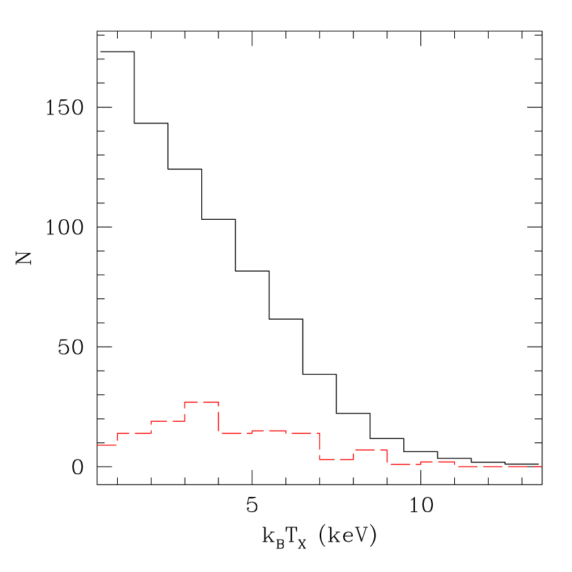
Figure 5: Expected cluster abundances in the nearby ($z\leq 0.2$) universe over 4.24 str (upper histogram), compared to the clusters used in our analysis (lower histogram). The expected abundance is estimated for an X-ray survey with flux limit and sky coverage similar to the REFLEX survey, using the concordant cosmological parameters. The comparison suggests that there are many more nearby clusters that can be added to our large sample, once their temperature is measured.

Turning to the future prospects, in the short term, the use of WMAP 4-year maps should decrease our errors on $f_{\rm gas}$ and concentration by a factor of $1.5-2$. Fig.(5) shows the estimated number of observed clusters with $z<0.2$, within different temperature bins, which is compared to the sample with measured temperatures used for this analyses. This shows that, even within the range of temperatures and redshifts resolved by WMAP, there are many more clusters that can be included in the analyses, if their temperatures are measured. Therefore, adding more clusters with observed X-ray temperatures to our catalog, e.g., from current and future Chandra observations, will increase the significance of our constraints.

In the long run, this work serves as an example to show the power of combining extragalactic observations in different frequencies in putting independent statistical constraints on the physical models of systems under study. More specifically, we have demonstrated that despite their low resolution, through combination with X-ray data, WMAP all-sky maps are capable of constraining the ICM physics at a comparable level of accuracy to their much higher-resolution pointed counterparts (e.g., OVRO and BIMA; see Grego et al., 2001) Therefore, we predict that the scientific outcome of future high resolution CMB/SZ observations (e.g., see Bond, 2002) will be greatly enhanced through direct combination/correlation with a wide-angle deep X-ray survey, such as NASA’s proposed Dark Universe Observatory (DUO) . It is needless to say that more accurate observational constraints on the ICM need to be supplemented by more sophisticated theoretical models which should be achieved through large and high-resolution numerical simulations. Such simulations are yet to be realized (see §5.3).

Appendix A An Analytic Model of the Intra-Cluster Medium

Numerical simulations indicate that the spherically averaged density distribution of dark matter, which also dominates the gravitational potential of galaxy clusters, may be well approximated by an NFW profile (Navarro, Frenk, & White, 1997, hereafter NFW)

$$\rho(r)=\frac{\rho_{s}}{(r/r_{s})(1+r/r_{s})^{2}}~{}{\rm,~{}for}~{}r<r_{\rm vir}=c_{\rm vir}~{}r_{s},$$ (A1)

where $\rho_{s}$ and $r_{s}$ are constants, and $c_{\rm vir}$, the so-called concentration parameter, is the ratio of $r_{\rm vir}$ to $r_{s}$. The virial radius, $r_{\rm vir}$, is defined as the boundary of the relaxed structure, generally assumed to be the radius of the sphere with an overdensity of $\Delta\simeq 200$ with respect to the critical density of the universe

$$\left(4\pi r_{\rm vir}^{3}\over 3\right)\left(\frac{3H^{2}}{8\pi G}\right)\Delta=M_{\rm vir}=\int^{c_{\rm vir}r_{s}}_{0}4\pi r^{2}dr\cdot\rho(r)=4\pi\rho_{s}r^{3}_{s}\left[\ln(1+c_{\rm vir})-{c_{\rm vir}\over 1+c_{\rm vir}}\right].$$ (A2)

Thus, fixing the mass of the cluster, $M_{\rm vir}$, and the concentration parameter, $c_{\rm vir}$, at a given redshift (which sets the critical density for given cosmology) fixes the dark matter profile ($\rho_{s}$ and $r_{s}$), and the associated gravitational potential

$$\phi(r)=-\frac{GM_{\rm vir}}{r}\cdot\frac{\ln(1+r/r_{s})}{\ln(1+c_{\rm vir})-c_{\rm vir}/(1+c_{\rm vir})}.$$ (A3)

To model the distribution of the diffuse gas in the Intra-Cluster Medium (ICM), following Suto et al. (1998), we assume that the gas follows a polytropic relation, i.e. $P_{g}(r)=\rho_{g}(r)T(r)/(\mu m_{p})\propto\left[\rho_{g}(r)\right]^{\gamma_{\rm eff}}$, and that it satisfies Hydrostatic equilibrium in the NFW potential, which reduces to

$$\frac{d}{dr}\left[T(r)+\mu m_{p}(1-\gamma_{\rm eff}^{-1})\phi(r)\right]=0.$$ (A4)

Here, $P_{g}(r)$, $\rho_{g}(r)$, and $T(r)$ are gas pressure, density, and temperature respectively, while $\gamma_{\rm eff}$ is the effective polytropic index of the gas and $m_{p}$ is the proton mass. $\mu=4/(3+5X)\simeq 0.59$ is the mean molecular weight for a cosmic hydrogen abundance of $X\simeq 0.76$ .

In order to integrate equation (A4), we need to set the boundary condition for $T(r)$. Assuming an accretion shock at $r_{\rm vir}$ (Voit et al., 2003), which causes the cold infalling gas to come to stop, the gas temperature behind the shock should be $T(r_{\rm vir})=\mu m_{p}v^{2}_{ac}/3$. In the spherical collapse model (Gunn, & Gott, 1972) $r_{\rm vir}\simeq 0.5\times r_{ta}$, the turn-around radius, which implies $v^{2}_{ac}=GM_{\rm vir}/r_{\rm vir}$, and respectively fixes $T(r)$

$$\frac{T(r)}{\mu m_{p}}\simeq-(1-\gamma_{\rm eff}^{-1})\left[\phi(r)-\phi(r_{\rm vir})\right]+\frac{GM_{\rm vir}}{3r_{\rm vir}}.$$ (A5)

Note that, as our SZ signal is dominated by the most massive clusters (see §5), it is a fair approximation to neglect the non-gravitational heating/cooling processes, which only become significant for smaller clusters (e.g., Voit et al., 2003). Both simulations and observations seem to indicate that $\gamma_{\rm eff}\simeq 1.2$ (e.g., FRB01, Voit et al., 2003; Borgani et al., 2004, and refernces therein), and thus, for the rest of our analyses, we will use this value. Also, simulations only predict a weak mass dependence for the concentration parameter, $c_{\rm vir}$ (e.g., NFW; Eke, Navarro, & Steinmetz, 2001; Dolag et al., 2004), and thus, for simplicity, we assume a mass-independent value of $c_{\rm vir}$. In §5 we explore the sensitivity of our observation on $c_{\rm vir}$.

Combining equations (A2),(A3), and (A5), we arrive at:

$$T(r)=\frac{\mu GM_{\rm vir}m_{p}}{r_{\rm vir}}~{}f(r/r_{\rm vir};c_{\rm vir},\gamma_{\rm eff}),$$ (A6)

where

$$f(x;c_{\rm vir},\gamma_{\rm eff})={1\over 3}+(1-\gamma_{\rm eff}^{-1})\left[\frac{\ln(1+c_{\rm vir}x)/x-\ln(1+c_{\rm vir})}{\ln(1+c_{\rm vir})-c_{\rm vir}/(1+c_{\rm vir})}\right],$$ (A7)

and

$$r_{\rm vir}=\left(\frac{2~{}GM_{\rm vir}}{H^{2}\Delta}\right)^{1/3}.$$ (A8)

The polytropic relation can be used to obtain the ICM gas density, $\rho_{g}(r)\propto[T(r)]^{1/(\gamma_{\rm eff}-1)}$, which yields

$$\rho_{g}(r)=f_{\rm gas}\left(\frac{M_{\rm vir}}{4\pi r_{\rm vir}^{3}}\right)g(r/r_{\rm vir};c_{\rm vir},\gamma_{\rm eff}),$$ (A9)

where

$$g(x;c_{\rm vir},\gamma_{\rm eff})=\frac{[f(x;c_{\rm vir},\gamma_{\rm eff})]^{1/(\gamma_{\rm eff}-1)}}{\int_{0}^{1}[f(y;c_{\rm vir},\gamma_{\rm eff})]^{1/(\gamma_{\rm eff}-1)}~{}y^{2}dy},$$ (A10)

and $f_{\rm gas}$ is the fraction of total mass in the ICM gas.

Now, let us obtain the observable quantities that are relevant to our study. Similar to previous works (e.g., Suto et al., 1998; Komatsu & Seljak, 2001), we approximate the observable X-ray temperature of clusters as the X-ray emission weighted gas temperature

$$T_{\rm x}\simeq\frac{\int T^{3/2}(r)\rho^{2}_{g}(r)~{}r^{2}dr}{\int T^{1/2}(r)\rho^{2}_{g}(r)~{}r^{2}dr}=\frac{\mu GM_{\rm vir}m_{p}}{r_{\rm vir}}~{}\frac{\int^{1}_{0}f^{3/2}(x)g^{2}(x)~{}x^{2}dx}{\int^{1}_{0}f^{1/2}(x)g^{2}(x)~{}x^{2}dx},$$ (A11)

which should be contrasted with the virial (mass-weighted) temperature

$$T_{\rm vir}=\frac{\int T(r)\rho_{g}(r)~{}r^{2}dr}{\int\rho_{g}(r)~{}r^{2}dr}=\frac{\mu GM_{\rm vir}m_{p}}{r_{\rm vir}}~{}\frac{\int^{1}_{0}f(x)g(x)~{}x^{2}dx}{\int^{1}_{0}g(x)~{}x^{2}dx}.$$ (A12)

As an example, for a nominal value of $c_{\rm vir}=3$, we find

$$T_{\rm x}=(8.7~{}{\rm keV})\left(\frac{M_{\rm vir}}{10^{15}h^{-1}{\rm\,M_{\odot}}}\right)^{2/3},{\rm~{}and~{}}T_{\rm vir}=(7.2~{}{\rm keV})\left(\frac{M_{\rm vir}}{10^{15}h^{-1}{\rm\,M_{\odot}}}\right)^{2/3},$$ (A13)

while, for $c_{\rm vir}=5$

$$T_{\rm x}=(9.9~{}{\rm keV})\left(\frac{M_{\rm vir}}{10^{15}h^{-1}{\rm\,M_{\odot}}}\right)^{2/3},{\rm~{}and~{}}T_{\rm vir}=(7.6~{}{\rm keV})\left(\frac{M_{\rm vir}}{10^{15}h^{-1}{\rm\,M_{\odot}}}\right)^{2/3}.$$ (A14)

We note that these relations are consistent, at the $10\%$ level, with the predictions of the universal gas profile model by Komatsu & Seljak (2001). Observations of X-ray mass-temperature relation are often expressed in terms of $M_{500}$, i.e. the mass enclosed inside the sphere with $\Delta=500$ (see equation A2). For $c_{\rm vir}=3(5)$, Equation (A2) gives $M_{500}/M_{\rm vir}=M_{500}/M_{200}=0.648(0.722)$ yielding

$$M_{500}(c_{\rm vir}=3{\rm~{}or~{}5})=(4.0{\rm~{}or~{}}3.7)\times 10^{13}h_{70}^{-1}{\rm\,M_{\odot}}\left(T_{\rm x}\over 5~{}{\rm keV}\right)^{3/2},$$ (A15)

corresponding to

$$M_{200}(c_{\rm vir}=3{\rm~{}or~{}5})=(6.2{\rm~{}or~{}}5.1)\times 10^{13}h_{70}^{-1}{\rm\,M_{\odot}}\left(T_{\rm x}\over 5~{}{\rm keV}\right)^{3/2},$$ (A16)

where $h_{70}\equiv h/0.7$. Borgani et al. (2004) argue that, on average, the beta model polytropic ($\beta\gamma$) mass estimates overestimate the normalization of the observed M-T relation by about $30\%$ at $\Delta=500$. Taking this into account, we notice that the normalization of the M-T relation in our model is consistent with the observations for hot clusters ($T_{\rm x}>2-3{\rm keV}$), at the $\sim 10\%$ level (e.g., see Table 3 in Arnaud et al., 2005). Therefore, we will use Equation (A11) to relate the observed X-ray temperatures of our clusters to their virial masses and radii. The expected systematic error in this conversion will be at the 10% level in mass estimates (or 3% in virial radii).

Figure 1: The distribution of cluster redshifts and virial radii (estimated from X-ray temperature, assuming $c_{\rm vir}=5$; see §3). The three upper lines show the resolution of WMAP bands (associated with the radius of the disk with the same effective area as the detector beams; see Page et al., 2003), while the lower line shows the physical radius of the 1 degree circle at the cluster redshift.

Figure 2: The binned values of gas fractions (solid circles/errorbars), inferred from our SZ measurements (assuming $c_{\rm vir}=3$ or $c_{\rm vir}=5$; Table 2). The solid triangles are the X-ray estimates for $f_{\rm gas}h$ (see the text), while the region enclosed by the dashed lines is the upper limit from the WMAP concordance model (Spergel et al., 2003).

Figure 3: The binned values of the average microwave luminosity per galaxy, $L_{PS}$, assuming a flat spectrum.

Figure 4: The $68\%$ and $95\%$ likelihood contours in the $f_{\rm gas}h-c_{\rm vir}$ plane for clusters with $T_{\rm x}>5~{}{\rm keV}$. The solid contours show the result from our SZ analysis, as described in the text. The dotted contours are for the $\Lambda$CDM concordance model, where $f_{\rm gas}h$ is from Spergel et al. (2003), while the concentration parameter and its uncertainty are obtained through the formalism developed in Afshordi & Cen (2002).

References

- Afshordi & Cen (2002) Afshordi, N. & Cen, R. 2002, ApJ, 564, 669
- Afshordi, Loh, & Strauss (2004) Afshordi, N., Loh, Y., & Strauss, M. A. 2004, Phys. Rev. D, 69, 083524
- Arnaud et al. (2005) Arnaud, M., Pointecouteau, E., & Pratt, G. W. 2005, ArXiv Astrophysics e-prints, astro-ph/0502210
- Bennett et al. (2003a) Bennett, C. L., et al. 2003, ApJS, 148, 1 (Bennett et al. 2003a)
- Bennett et al. (2003b) Bennett, C. L., et al. 2003, ApJS, 148, 97 (Bennett et al. 2003b)
- Benson et al. (2004) Benson, B. A., Ade, P. A. R., Bock, J. J., Ganga, K. M., Henson, C. N., Thompson, K. L., & Church, S. E. 2004, ArXiv Astrophysics e-prints, astro-ph/0404391
- Bialek, Evrard, & Mohr (2001) Bialek, J. J., Evrard, A. E., & Mohr, J. J. 2001, ApJ, 555, 597
- Bond (2002) Bond, J. R. 2002, ASP Conf. Ser. 257: AMiBA 2001: High-Z Clusters, Missing Baryons, and CMB Polarization, 327
- Borgani et al. (2004) Borgani, S., et al. 2004, MNRAS, 348, 1078
- Bryan (2000) Bryan, G. L. 2000, ApJ, 544, L1
- Bullock et al. (2001) Bullock, J. S., Kolatt, T. S., Sigad, Y., Somerville, R. S., Kravtsov, A. V., Klypin, A. A., Primack, J. R., & Dekel, A. 2001, MNRAS, 321, 559
- Carlstrom, Holder, & Reese (2002) Carlstrom, J. E., Holder, G. P., & Reese, E. D. 2002, ARA&A, 40, 643
- Cen & Ostriker (1999) Cen, R. & Ostriker, J. P. 1999, ApJ, 514, 1
- Chieze, Alimi, & Teyssier (1998) Chieze, J., Alimi, J., & Teyssier, R. 1998, ApJ, 495, 630
- Cooray et al. (1998) Cooray, A. R., Grego, L., Holzapfel, W. L., Joy, M., & Carlstrom, J. E. 1998, AJ, 115, 1388
- Cooray (1999) Cooray, A. R. 1999, MNRAS, 307, 841
- David et al. (1993) David, L. P., Slyz, A., Jones, C., Forman, W., Vrtilek, S. D., & Arnaud, K. A. 1993, ApJ, 412, 479
- Diaferio et al. (2004) Diaferio, A., et al. 2004, ArXiv Astrophysics e-prints, astro-ph/0405365
- Dolag et al. (2004) Dolag, K., Bartelmann, M., Perrotta, F., Baccigalupi, C., Moscardini, L., Meneghetti, M., & Tormen, G. 2004, A&A, 416, 853
- Eke, Cole, & Frenk (1996) Eke, V. R., Cole, S., & Frenk, C. S. 1996, MNRAS, 282, 263
- Eke, Navarro, & Steinmetz (2001) Eke, V. R., Navarro, J. F., & Steinmetz, M. 2001, ApJ, 554, 114
- Evrard (1997) Evrard, A. E. 1997, MNRAS, 292, 289
- Finoguenov, Reiprich, & Böhringer (2001) Finoguenov, A., Reiprich, T. H., & Böhringer, H. 2001, A&A, 368, 749 (FRB01)
- Fosalba, Gaztañaga, & Castander (2003) Fosalba, P., Gaztañaga, E., & Castander, F. J. 2003, ApJ, 597, L89
- Fosalba & Gaztañaga (2004) Fosalba, P. & Gaztañaga, E. 2004, MNRAS, 350, L37
- Fox & Loeb (1997) Fox, D. C. & Loeb, A. 1997, ApJ, 491, 459
- Górski, Hivon, & Wandelt (1999) Górski, K. M., Hivon, E., & Wandelt, B. D. 1999, Evolution of Large Scale Structure : From Recombination to Garching, 37; http://www.eso.org/science/healpix/
- Goto et al. (2003) Goto, T., Yamauchi, C., Fujita, Y., Okamura, S., Sekiguchi, M., Smail, I., Bernardi, M., & Gomez, P. L. 2003, MNRAS, 346, 601
- Grego et al. (2001) Grego, L., Carlstrom, J. E., Reese, E. D., Holder, G. P., Holzapfel, W. L., Joy, M. K., Mohr, J. J., & Patel, S. 2001, ApJ, 552, 2
- Gunn, & Gott (1972) Gunn, J. E. & Gott, J. R. I. 1972, ApJ, 176, 1
- Haiman, Mohr, & Holder (2001) Haiman, Z., Mohr, J. J., & Holder, G. P. 2001, ApJ, 553, 545
- Hennawi & Spergel (2004) Hennawi, J. F. & Spergel, D. N. 2004, ArXiv Astrophysics e-prints, astro-ph/0404349
- Henry (2000) Henry, J. P. 2000, ApJ, 534, 565
- Henry (2004) Henry, J. P. 2004, ApJ, 609, 603