Multifrequency Analysis of 21 cm fluctuations From the Era of Reionization

Abstract

We study the prospects for extracting detailed statistical properties of the neutral Hydrogen distribution during the era of reionization using the brightness temperature fluctuations from redshifted 21 cm line emission. Detection of this signal is complicated by contamination from foreground sources such as diffuse Galactic synchrotron and free-free emission at low radio frequencies, extragalactic free-free emission from ionized regions and radio point sources. We model these foregrounds to determine the extent to which 21 cm fluctuations can be detected with upcoming experiments. We find that not only the level of correlation from one frequency to another, but also the functional form of the foreground correlations has a substantial impact on foreground removal. We calculate how well the angular power spectra of the 21cm fluctuations can be determined. We also show that the large-scale bias of the neutral Hydrogen gas distribution with respect to the density field, can be determined with high precision and used to distinguish between different reionization histories.

1 Introduction

Recently there has been a great deal of interest in the reionization of the intergalactic medium (Cen, 2003; Chen et al., 2003; Cen & McDonald, 2002; Gnedin, 2004; Wyithe & Loeb, 2003; Haiman & Holder, 2003; Sokasian et al., 2003; Miralda-Escudé et al., 2000). This interest was sparked by the detection (Bennett et al., 2003; Kogut et al., 2003) of a correlation between polarization and temperature on large angular scales (Zaldarriaga, 1997). The amplitude of the signal suggests that reionization began much earlier than $z\sim 6$, which is when the inter-galactic medium became completely ionized as we know from the detection of Gunn-Peterson troughs (Gunn & Peterson, 1965; Becker et al., 2001; Fan et al., 2002).

Now that the ionization history appears to be quite rich, we wish to study the epoch in detail. Unfortunately, the CMB is mostly sensitive only to the integral history of reionization. Although different reionization histories with the same optical depth do give different large angular scale polarization power spectra, one cannot easily use these changes to fully reconstruct the reionization history as a function of redshift due to the large cosmic variance on large angular scales (Kaplinghat et al., 2003; Hu & Holder, 2003; Haiman & Holder, 2003).

Another way to study the reionization history of the Universe in more detail is through the observation of the distribution of neutral Hydrogen based on the spin-flip transition at a rest wavelength of 21 cm. Plans for upcoming low-frequency radio experiments such as PAST (Pen et al., 2004), Mileura Widefield Array (MWA), Low Frequency Array (LOFAR) and Square Kilometer Array (SKA) have now motivated detailed study of the 21 cm background associated with neutral hydrogen during, and prior to, reionization (e.g., Scott & Rees 1990; Madau et al. 1997; Gnedin & Ostriker 1997; Zaldarriaga et al. 2004; Morales & Hewitt 2003; Kumar et al. 1995; Tozzi et al. 2000; Iliev et al. 2002; Bharadwaj & Ali 2005). Unlike the CMB, the advantage here is that by a priori selecting the observed frequency, one can probe the neutral content of the Universe at a given redshift, thereby obtaining a tomographic view of the reionization process. This way, one can reconstruct the reionization history and determine, especially, if the reionization process was either instantaneous or lengthy and complex as implied by current CMB data. Moreover, since observable effects in CMB data depend only on the ionized content while 21 cm fluctuations come from inhomogeneities in the neutral distribution, the combination may allow additional information in the study of reionization.

Although there is strong scientific motivation to study 21 cm fluctuations during the era of reionization, there are several difficulties to overcome. In addition to experimental challenges, involving observations at low radio frequencies, the background itself is highly contaminated by foreground radio emission. Synchrotron and free-free emission from the Milky Way (Shaver et al., 1999), low frequency radio point sources (Di Matteo et al., 2002, 2004) and free-free emission from free electrons in the intergalactic medium (Oh, 1999; Cooray & Furlanetto, 2004) are now thought to be the chief sources of confusion. While it has been suggested (Oh & Mack, 2003) that background studies may be impossible due to the large number of contaminating sources (with brightness fluctuations much higher than expected for neutral Hydrogen at high redshifts), others have contended that a multifrequency analysis of the 21 cm data can be used to reduce the foreground contamination given the smoothness of these contaminants in frequency space (Shaver et al., 1999; Di Matteo et al., 2002; Zaldarriaga et al., 2004). Initial calculations suggest that, for experiments such as LOFAR and SKA, one can easily remove the foregrounds to a sufficiently low level that statistical studies related to 21 cm fluctuations can be achieved (Zaldarriaga et al., 2004).

In this paper, we extend the initial discussions related to foreground removal by considering a detailed analysis of the multifrequency removal technique. When estimating how accurately cosmological parameters can be measured, we take into account the complication that most foreground properties, like the level of smoothness across frequency, must be estimated at the same time as the signal. Our foreground model includes not only the normalization, frequency dependence and scale dependence for each physical quantity, but also variations in the frequency coherence and even the functional form of the foreground correlations across frequency. We also consider the extent to which 21 cm fluctuations can be cross-correlated between frequency bins. This cross-correlation of the signal between channels reduces the efficiency with which foregrounds can be cleaned.

The paper is organized as follows: in §2, we discuss the 21 cm signal anisotropy and frequency correlations. In §3, we give an overview of the most important foreground contaminants. In §4 we discuss the experimental setup assumed in our analysis. In §5 we discuss the method used for the error forecast and the multifrequency cleaning techniques to reduce the foreground contamination. Finally in §6 we study how well physical parameters related to the 21 cm signal can be extracted. Throughout the paper, we make use of the WMAP-favored $\Lambda$CDM cosmological model (Spergel et al., 2003).

2 The 21cm signal

When traveling through a patch of neutral hydrogen, the intensity of the CMB radiation will change due to absorption and emission. The corresponding change in the brightness temperature, $T_{21}(\nu)$, as compared to the CMB at an observed frequency $\nu$ is then

$$T_{21}(\nu) \approx \frac{T_{S}-T_{\rm CMB}}{1+z}\,\tau$$ (1)

where $T_{S}$ is the temperature of the source (the spin temperature of the IGM), $z$ is the redshift corresponding to the frequency of observation ($1+z=\nu_{21}/\nu$, with $\nu_{21}=1420$ MHz) and $T_{\rm CMB}=2.73(1+z)K$ is the CMB temperature at redshift $z$. The optical depth, $\tau$, of this patch in the hyperfine transition (Field, 1959) is given in the limit of $k_{B}T_{s}>>h\nu_{21}$ by

$$\tau = \frac{3c^{3}\hbar A_{10}\,n_{\rm HI}}{16k\nu_{21}^{2}\,T_{S}\,H(z)}$$ (2)

$$\approx 8.6\times 10^{-3}(1+\delta_{b})x_{H}\left[\frac{T_{\rm CMB}(z)}{T_{S}}\right]\left(\frac{\Omega_{b}h^{2}}{0.02}\right)$$

$$\times\left[\left(\frac{0.15}{\Omega_{m}h^{2}}\right)\,\left(\frac{1+z}{10}\right)\right]^{1/2}\left(\frac{h}{0.7}\right)^{-1},$$

where $A_{10}$ is the spontaneous emission coefficient for the transition ($2.85\times 10^{-15}$ s^-1) and $n_{\rm HI}$ is the neutral hydrogen density. This can be expressed as $n_{\rm HI}=x_{H}\bar{n}_{b}(1+\delta_{b})$, when $\bar{n}_{b}$ is the mean number density of cosmic baryons, with a spatially varying overdensity $\delta_{b}$ and $x_{H}$ is the fraction of neutral hydrogen ($x_{H}=1-x_{e}$ where $x_{e}$ is the fraction of free electrons). We refer the reader to Zaldarriaga et al. (2004) for further details.

2.1 21cm Power Spectrum

The measured brightness temperature corresponds to a convolution of the intrinsic brightness with some response function $W_{\nu}(r)$ that characterizes the bandwidth of the experiment:

$$T^{s}({\bf\hat{n}},\nu_{0})=\int drW_{\nu_{0}}(r)T_{21}({\bf\hat{n}},r),$$ (3)

where ${\bf\hat{n}}$ is the direction of observation and $r$ is the radial distance corresponding to the observed frequency $\nu$. We can now determine the angular power spectrum of $T^{s}({\bf\hat{n}},\nu_{0})$ which is related to the 3-d power spectrum of $T_{21}({\bf\hat{n}},r)$, defined by

$$\langle\tilde{T}_{21}({\bf k},\nu_{1})\tilde{T}_{21}({\bf k}^{\prime},\nu_{2})\rangle=(2\pi)^{3}\delta^{D}({\bf k}+{\bf k}^{\prime})P_{21}(k,\nu_{1},\nu_{2}),$$ (4)

where $T_{21}({\bf\hat{n}},r)\equiv T_{21}({\bf r},\nu)=\int{d^{3}k\over(2\pi)^{3}}\tilde{T}_{21}({\bf k},\nu)e^{i{\bf k}\cdot{\bf r}}$. Making use of the spherical harmonic moment of the 21 cm fluctuations, at a frequency $\nu_{0}$,

$$a^{s}_{lm}(\nu_{0})=\int d{\bf\hat{n}}Y^{*}_{lm}({\bf\hat{n}})T^{s}({\bf\hat{n}},\nu_{0})\,,$$ (5)

we write the angular power spectrum as (e.g. Kaiser 1992)

$$\langle a^{s}_{lm}(\nu_{1})a^{s*}_{lm}(\nu_{2})\rangle=C^{s}_{l}(\nu_{1},\nu_{2})$$ (6)

$$={2\over\pi}\int k^{2}dk\,P_{21}(k,\nu_{1},\nu_{2})I_{l}^{\nu_{1}}(k)I_{l}^{\nu_{2}}(k)\,,$$

where

$$I_{l}^{\nu}(k)=\int drW_{\nu}(r)j_{l}(kr)\,,$$ (7)

with the spherical Bessel function given by $j_{l}(kr)$. In deriving this form for the angular power spectrum, we have made use of the Rayleigh expansion for the plane wave given by

$$e^{i{\bf k}\cdot{\bf r}}=4\pi\sum_{lm}i^{l}j_{l}(kr)Y_{l}^{m}({\bf\hat{n}})Y_{l}^{m*}(\hat{{\bf k}})\,.$$ (8)

In Figure 1, we show in the top panel the integral, $I_{l}^{\nu}(k)$, when $l=100$ as a function of $k$, for three different frequency bins of width 1MHz. As the frequency separation increases, the oscillations are out of phase suggesting that $C^{s}_{l}(\nu_{1},\nu_{2})$ is not significant for $\nu_{2}-\nu_{1}\gg 10{\rm MHz}$.

Figure 1: The frequency cross-correlations of the 21cm signal. Top panel: the absolute value of the function $I_{l}^{\nu}(k)$ when $l=100$ for three frequency bins with a width of 1MHz. For large frequency separations these functions are out of phase and the integral over k is essentially zero. Bottom panel: signal correlations across frequency. Each curve corresponds to a frequency separation from 1MHz to 10MHz (1MHz bandwidth).

However, for smaller separations $C^{s}_{l}(\nu_{1},\nu_{2})$ certainly cannot be considered to be zero. This is clear by looking at the bottom panel of Figure 1 where we show the signal correlations across frequency for separations from 1 to 10MHz.

To proceed further we need an expression for the power spectrum of the 21 cm fluctuations, $P_{21}(k,z)$, or in this case, spatial inhomogeneities in the underlying gas density field. In order to simplify the calculation related to fluctuations in the density field, we assume a scenario where the gas density field is heated well above the CMB temperature during the reionization process. In addition to reionization, we also expect the structure formation process, such as shocks in forming virialized dark matter halos, where first stars eventually form to subsequently reionize the universe, to heat the gas such that $T_{s}\gg T_{CMB}$ (Gnedin & Shaver, 2004). The gravitational shocks will also heat the gas in overdense regions like sheets and filaments such that the assumption we make here with regards to the gas temperature should be valid throughout the IGM at a time around the era of reionization where one also expects a substantial background of X-rays from supernovae, etc (Venkatesan et al., 2001; Chen & Miralda-Escudé, 2004) to also heat the IGM quickly. At sufficiently high $z$, prior to significant reionization and heating, we expect $T_{s}<T_{\rm CMB}$ and it may be possible to see HI in 21cm absorption (Madau et al., 1997).

With $T_{s}>>T_{\rm CMB}$, the 21 cm signal will be observed in emission with respect to the background CMB. Writing the brightness temperature as:

$$T_{21}(z)=c\,(1+\delta)(1-\bar{x}_{e}-\bar{x}_{e}\delta_{x}),$$ (9)

where

$$c\approx 23\left(\frac{\Omega_{b}h^{2}}{0.02}\right)\\ \left[\left(\frac{0.15}{\Omega_{m}h^{2}}\right)\,\left(\frac{1+z}{10}\right)\right]^{1/2}\left(\frac{h}{0.7}\right)^{-1}{\rm mK}$$

and $\delta_{x}$ is the perturbation in the ionization fraction ($\delta_{x}\equiv{x_{e}-\bar{x}_{e}\over\bar{x}_{e}}$), the corresponding three-dimensional power spectrum is

$$P_{21}(k,z) = c^{2}\left[(1-\bar{x}_{e})^{2}P_{\delta\delta}(k,z)+\bar{x}_{e}^{2}P_{\delta_{x}\delta_{x}}(k,z)\right.$$ (10)

$$- \left.2P_{\delta\delta_{x}}(k,z)\bar{x}_{e}(1-\bar{x}_{e})\right].$$

The dark matter power spectrum is represented by $P_{\delta\delta}(k,z)$ (and we are assuming that $\delta=\delta_{b}$), $P_{\delta_{x}\delta_{x}}(k,z)$ is the power spectrum from the perturbations in the ionized fraction and $P_{\delta\delta_{x}}(k,z)$ is the cross-correlation power.

The correlations in the ionized fraction depend on the reionization history. To proceed further we used the model of patchy reionization in Santos et al. (2003a) to write

$$P_{\delta_{x}\delta_{x}}(k,z)=b^{2}(z)P_{\delta\delta}(k,z)e^{-k^{2}R^{2}}$$ (11)

where $b(z)$ is a mean bias (halo bias weighted by the different halo properties) and $R$ the mean radius of the HII patches.

We crudely model the time-dependence of $R$ as $R=\left({1\over 1-\bar{x}_{e}}\right)^{1/3}R_{p}$ where $R_{p}$ is the (comoving) size of the fundamental patch which we take to be $R_{p}\sim 100$ Kpc. The cutoff scale $R$ is equal to $R_{p}$ when reionization starts and increases with time as HII regions overlap and form larger HII regions. The dependence of $R/R_{p}$ on $\bar{x}_{e}$ follows from assuming a Poisson distribution of patches and that their volumes add when they overlap. The essential consequence of this dependence of $R$ on $x_{e}$ and our choice of $R_{p}$ is that for $l\lesssim 10,000$ (scales greater than 1 Mpc) the transition is very sudden; i.e., $R$ increases from 1 Mpc to $\infty$ very rapidly.

In reality there is a distribution of patch sizes and there are spatial correlations between ionizing sources which cause some of the patches to overlap earlier than they would given a Poisson distribution. Furlanetto et al. (2004b) have recently developed a sophisticated model of the size distribution of patches and their correlations. They find a much more gradual transition to large patch sizes. In their model, large patch sizes suppress fluctuation power even as low as $l=1000$ while the ionization fraction is still as low as $\bar{x}_{e}=0.5$ (although this depends on the assumed efficiency with which the collapsed baryons ionize the surrounding hydrogen). We caution the reader that modeling the signal on scales smaller than the largest patches is difficult and the shape of the signal on these scales remains highly uncertain.

The bias in equation 11 is much larger than 1 so that we can safely neglect the cross-correlation contribution in our analysis. We show in Figure 2 the 21cm power spectra for three reionization models with the same optical depth ($\tau=0.17$). Typically, for $z>7$ the reionization models give $R\sim 0.2$Mpc so that the size of the patches are only important for $l>10^{4}$ and below that, the power spectrum just follows the shape of the matter density perturbations. Note that the bend in the curves at $l\sim r/\delta r\sim 500$, where $\delta r$ is the width of the window function, $W_{\nu}(r)$, is due to the Limber regime where perturbations are smoothed out. Figures 3 and 4 show the ionization fraction and bias for the corresponding reionization models from Haiman & Holder (2003).

Figure 2: The power spectrum for the 21cm signal at z=9.2 and assuming a bandwidth of $\Delta\nu=1$MHz. The solid, dashed and dot-dashed lines use the corresponding reionization models shown in Figures 3 and 4.

Figure 3: $\bar{X}_{e}$ for three different fiducial models with $\tau=0.17$. Solid line is for the fiducial model used throughout the paper. Dashed line assumes that $H_{2}$ feedback effectively shuts off star formation in all Type II halos. Dot-dashed line assumes that a transition from metal free to normal star formation takes place abruptly at a certain redshift.

Figure 4: Effective bias for the same fiducial models as in Figure 3.

3 Foregrounds

We consider four different foregrounds: Galactic synchrotron, Galactic free-free, extra-galactic diffuse free-free and extra-galactic point sources. All of these contaminants produce much more fluctuation power at each frequency than the 21cm signal. Measurement of the 21cm signal would be impossible if not for the high coherence of the contaminants across frequency, compared to the very short frequency space correlation length of the signal.

With $i$ and $j$ labeling the different contaminants let us define

$$C_{l}^{ij}(\nu_{1},\nu_{2})\equiv\langle a_{lm}^{i}(\nu_{1})a_{lm}^{j}(\nu_{2})\rangle.$$ (12)

We expect correlations between the different contaminants to be negligible. We model the foregrounds as power laws in both $l$ and $\nu$ so that:

$$C_{l}^{ii}(\nu,\nu)=A_{i}(1000/l)^{\beta_{i}}(\nu_{f}/\nu)^{2\bar{\alpha}_{i}}.$$ (13)

where $\nu_{f}=130{\rm MHz}$. We also expect the foregrounds to be highly coherent, i.e. $I_{l}^{ii}(\nu_{1},\nu_{2})\simeq 1$ where

$$I_{l}^{ii}(\nu_{1},\nu_{2})\equiv C_{l}^{ii}(\nu_{1},\nu_{2})/\sqrt{C_{l}^{ii}(\nu_{1},\nu_{1})C_{l}^{ii}(\nu_{2},\nu_{2})}.$$ (14)

Although we consider other parameterizations of $I_{l}^{ii}$, our starting point is

$$I_{l}^{ii}(\nu_{1},\nu_{2})=exp\left[-\log^{2}(\nu_{1}/\nu_{2})/2/\xi_{ii}^{2}\right],$$ (15)

which, for the frequency range and values of $\xi_{ii}$ we will be considering, reduces to

$$I_{l}^{ii}(\nu_{1},\nu_{2})\sim 1-\log^{2}(\nu_{1}/\nu_{2})/2/\xi_{ii}^{2}.$$ (16)

This form describes the departure from complete correlation to lowest non-trivial order. It follows if one assumes the underlying sources have power-law spectra with varying spectral indices $\alpha$. If sources with different spectral indices have $C_{l}$’s with different shapes (for example, because they have different redshift distributions), then $I_{l}$ can be $l$-dependent. Note that, due to this decorrelation, the frequency dependence of the foreground brightness temperature will actually have departures from a power law and change with position on the sky.

If $C_{l}$ is dominated by Poisson fluctuations, then $\xi=1/\Delta\alpha$ where $\Delta\alpha=\langle(\alpha-\bar{\alpha})^{2}\rangle^{1/2}$. This was the case considered by Tegmark (1998). If $C_{l}$ is dominated by clustering and $d\ln C_{l}/d\ln\alpha=0$ then $\xi=\sigma_{\alpha}/\Delta\alpha^{2}$ where, following Zaldarriaga et al. (2004), we assume that correlations between sources with $\alpha_{1}$ and $\alpha_{2}$ fall off as $\exp{[-(\alpha_{1}-\alpha_{2})^{2}/(2\sigma_{\alpha}^{2})]}$.

In Table 1 we show the parameters of our fiducial models for the four different contaminants that we now discuss. Figure 5 shows the expected foreground power spectrum together with the signal at 140MHz.

	$A({\rm mK}^{2})$	$\beta$	$\bar{\alpha}$	$\xi$
extragalactic point sources	57.0	1.1	2.07	1.0
extragalactic free-free	0.014	1.0	2.10	35
Galactic synchrotron	700	2.4	2.80	4.0
Galactic free-free	0.088	3.0	2.15	35

Table 1: Fiducial parameters at $l=1000$ and $130$MHz. Parameters are defined in equations 13,  14 and 15.

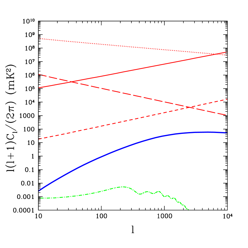
Figure 5: The 21cm power spectrum (blue thick line) at z=9.2 ($\nu=140$ MHz) and its foregrounds. Point sources - red thin solid line, Galactic Synchrotron - red thin dotted line, Extragalactic free-free - red thin dashed line and Galactic free-free - red thin long-dashed line. CMB - green dot-dashed line.

3.1 Extragalactic point sources

The extragalactic sources of contamination likely to be important at the relevant low flux levels are radio galaxies, active galactic nuclei and normal galaxies. There are several surveys of extragalactic sources in or near the wavelength range of interest including the 6C survey (Hales et al., 1988) at 151 MHz, the 3CR survey at 178 MHz (Laing et al., 1983) and a survey by Cohen et al. (2004) at 74 MHz.

All but the Cohen et al. (2004) survey were used by Di Matteo et al. (2002) to estimate the angular power spectra from unresolved sources at 150 MHz. They model both the Poisson contribution and the correlated contribution, assuming the sources are clustered like Lyman break galaxies (Giavalisco et al., 1998) at $z\sim 3$. They find that if sources brighter than $S_{\rm cut}=0.1$ Jy can be detected and removed, then the clustering signal, and not the Poisson signal, will be the dominant contribution to the variance of maps smoothed on angular scales larger than about 1’. As the flux cut is reduced further, the Poisson contribution drops faster than the clustering contribution, due to the Poisson contribution’s heavier weighting of the brightest sources.

We use the Di Matteo et al. (2002) model with $S_{\rm cut}=0.1$ mJy for the angular power spectrum of the background of unresolved sources . This translates into $A=57{\rm mK}^{2}$, and $\beta=1.1$ as shown in Table 1.

For the frequency dependence we turn to Cohen et al. (2004) who compare fluxes of 947 of their 949 sources that appear also in the NVSS survey at 1400 MHz (Condon et al., 1998). Assuming the spectrum of each source follows a power-law in intensity, $I_{\nu}\propto\nu^{\gamma}$, they find an average power-law index of $\bar{\gamma}^{1400}_{74}=-0.79$ with a scatter of about $\delta\gamma=0.2$. They also see a trend for flattening of spectral index as the 74 MHz flux density drops from 1 Jy down to 0.2 Jy going roughly as

$$\bar{\gamma}^{1400}_{74}=-0.83-0.13\log_{10}\left(I_{74}/{\rm Jy}\right).$$ (17)

Extrapolating further down to 0.1 mJy we find $\bar{\gamma}^{1400}_{74}=-0.31$.

Cohen et al. (2004) also find 545 of the 947 sources in the WENSS catalog at 325 MHz (Rengelink et al., 1997). They find a significant flattening of the spectra of most sources towards lower frequencies. The mean spectral indices are related by $\bar{\gamma}^{325}_{74}=0.24+\bar{\gamma}^{1400}_{74}=-0.07$.

Since fluctuations in antenna temperature follow as $\delta T(\nu)\propto\nu^{-2}\delta I_{\nu}$, then $\bar{\alpha}=2-\bar{\gamma}$. Our best guess based on the extrapolations to lower flux densities and lower frequencies is that $\bar{\gamma}=-0.07$ and therefore we use $\bar{\alpha}=2.07$ as our fiducial value.

Since clustering, according to Di Matteo et al. (2002), is the dominant source of fluctuation power we have $\xi=\sigma_{\alpha}/\Delta\alpha^{2}$. For our fiducial model we take $\Delta\alpha=\delta\gamma=0.2$, consistent with Cohen et al. (2004). The value for $\sigma_{\alpha}$ is less clear. As Zaldarriaga et al. (2004) argue, if the sources are all tracing the same dark matter distribution, even with different biases, then they would be perfectly correlated with each other; i.e., $\sigma_{\alpha}=\infty$. Certainly on large scales we expect this to be a good approximation. In the context of the halo model (Cooray & Sheth, 2002), the relevant length scale is the size of a typical halo hosting these sources. How this translates to an angular scale depends on distance to the source.

We have not attempted to calculate $\sigma_{\alpha}$ here, but merely point out that even taking the conservative assumption that $\sigma_{\alpha}=\Delta\alpha$ we get $\xi=5$. Because, as we will see, we can afford to be even more conservative, we set our fiducial value of $\xi$ even smaller to $\xi=1$.

We note that although for low $S_{\rm cut}$ clustering may be the dominant source of fluctuation power, Poisson fluctuations may remain as the dominant source of decorrelation, especially if $\sigma_{\alpha}>>\Delta\alpha$. In this case though, $\xi$ would still be greater than $1/\Delta\alpha$ and therefore even more coherent than in our fiducial model.

We also note that although the extrapolations from current observations of sources in the relevant wavelengths are over many decades in intensity, we are, of course, not stuck with these extrapolations. With the type of experiments we consider here, we will be able to study large numbers of resolved sources with flux densities just above $S_{\rm cut}$.

3.2 Extragalactic free-free emission

The low-frequency radio background produced by ionized electrons, via the free-free emission, is known to be a significant foreground for 21 cm studies (Oh, 1999; Oh & Mack, 2003; Cooray & Furlanetto, 2004). The free-free emission coefficient can be written as

$$\epsilon_{\nu} = 5.4\times 10^{-39}n_{e}^{2}T_{e}^{-1/2}g_{ff}(\nu,T_{e})e^{-h\nu/kT_{e}}$$ (18)

$$\quad\quad\quad\,{\rm ergs\;cm^{-3}\;s^{-1}\;Hz^{-1}\;sr^{-1}}\,,$$

where the Gaunt factor can be approximated in the radio regime as $g_{ff}(\nu,T_{e})\approx 11.96T_{e}^{0.15}\nu^{-0.1}$ (Lang, 1999). The cumulative specific intensity is simply $I_{\nu}=\int d\chi\epsilon_{\nu}(z)\bar{x}_{e}^{2}(z)\\ C(z)/(1+z)^{4}$, where $\chi$ is the conformal time and $\nu(z)=\nu_{\rm obs}(1+z)$ with $\nu_{\rm obs}$ the observed frequency. The brightness temperature is $T_{b}=c^{2}I_{\nu}/2\nu^{2}_{\rm obs}k_{B}$ and the electron fraction $\bar{x}_{e}(z)$ captures the mean ionization history of the IGM. The clumping factor of the electron density field is defined as $C(z)=\langle n_{e}^{2}\rangle/\langle n_{e}\rangle^{2}$. When estimating the free-free background and its spatial fluctuations, this is the most uncertain parameter. Initial estimates of the free-free background suggest that gas clumping boosts the specific intensity by a factor from order unity at $z\sim 20$ to over 100 at $z\lesssim 3$ (Oh, 1999).

A variety of models from the literature considered in Cooray & Furlanetto (2004) suggest that the free-free background is uncertain by at least 2 orders of magnitude. Among these models, a favorite is to estimate the clumping from the large-scale matter distribution by, for example, assuming that ionized electrons reside in virialized dark matter halos (Haiman et al., 2001; Benson et al., 2001; Gnedin & Ostriker, 1997) though such models are only expected to yield a minimal estimate for $C(z)$, because the models do not include recombinations within galaxies (where most ionizing photons are probably absorbed) or the biased distribution of ionizing sources. Numerical simulations by Gnedin (2000) show that these two factors strongly affect the effective clumping factor early in the reionization process, when ionizing photons are confined to the dense regions around galaxies. The second approach, taken by Oh (1999), is to construct a model for the production rate of ionizing photons $\dot{n}_{\rm ion}$ and assume that, throughout the universe, ionization equilibrium is a good approximation. The quantity $\bar{x}_{e}^{2}C(z)$ is then fixed through the relation

$$\dot{n}_{\rm ion}=\bar{x}_{e}^{2}(z)n_{e}^{2}(z)C(z)\alpha_{\rm rec},$$ (19)

where $\alpha_{\rm rec}$ is the recombination coefficient. This approach predicts stronger clumping than models based on the IGM gas as it includes recombinations inside galaxies. These dominate the clumping so long as the escape fraction of ionizing photons is small. However, this method depends on the assumed (and uncertain) ionizing photon production rate. It also does not include collisional ionization in massive halos at low redshift, though this is expected to be small.

The results related to these two approaches and a comparison to results from numerical estimates of gas clumping are summarized in Cooray & Furlanetto (2004). In Fig. 5, we make use of the high-end estimate of free-free anisotropy spectrum based on a model related to ionization equilibrium and using the star-formation history derived by Hernquist & Springel (2003). In addition to the angular power spectrum, the foreground model requires information related to the coherence of fluctuations between frequencies. Given that the extragalactic free-free emission is dominated by point sources at $z\sim 3$ which follow a biased distribution with respect to the linear density field, the angular power spectrum is dominated by the clustering nature of this point source distribution. The parameter of interest, $\xi$, then takes the value of $\sigma_{\alpha}/\Delta\alpha^{2}$ where $\alpha$ is the frequency dependence determined by a combination of the Gaunt factor and e${}^{-h\nu/kT_{e}}$. Even accounting for variations in the electron temperature by an order of magnitude, from 10⁴ to 10⁵ K, the spectral index, as a function of frequency, varies slowly, since $h\nu\ll kT_{e}$. We take this small variations into account by setting $\xi=35$ (with $\Delta\alpha\sim 0.03$ assuming $\sigma_{\alpha}\approx\Delta\alpha$). This value is significantly high when compared to, say, radio point sources with a value of $\xi=1$ in our fiducial model. The difference is due to the fact that observed spectral indices of point sources are rapidly varying from one source to another while free-free frequency spectra, from source to source, is expected to be very uniform due to the nature of free-free emission.

While the anisotropy spectrum and frequency coherence are just estimates based on model calculations, unfortunately, there are no observational measurements of the free-free background either in terms of mean brightness temperature or spatial fluctuations. The planned Absolute Radiometer for Cosmology, Astrophysics, and Diffuse Emission (ARCADE) experiment may be able to study some aspects of free-free background at frequencies around a few GHz. Also, low-frequency experiments such as SKA will have a high frequency imaging capabilities such that one can use data at frequencies just above 1420 MHz to determine the extent to which free-free emission can be a contaminant at low radio frequencies. While the free-free background can be a problem, in Cooray & Furlanetto (2004) it was shown that the integrated signal is dominated by low-$z$ sources (at redshifts less than 3). Also, a large fraction of the free-free fluctuations comes from relatively bright point sources that can be cleaned from the maps. Given that most of the emission is at low redshifts, when compared to 21 cm fluctuations from the reionization era, the free-free spectrum is smooth in frequency. Thus, multi-frequency differencing is expected to remove the smooth background radiation but not 21 cm radiation as the two fields are strongly uncorrelated given the disjoint in redshift distributions; we do expect some free-free emission from the era of reionization, but this was shown to be substantially below the noise level of upcoming experiments in Cooray & Furlanetto (2004).

If the fraction of emission at $z\sim 10$ were to be higher for some reason, then the confusion with free-free fluctuations may become substantial; for free-free fluctuations to dominate 21 cm anisotropies, even with optimal multifrequency cleaning, we require the fractional contribution to total emission from $z\sim 10$ to be at the same level as $z\sim 1$, which we do not consider to be physically possible. Thus, it is unlikely that after multifrequency cleaning, free-free fluctuations will be the dominant residual contamination of 21 cm maps.

3.3 Galactic Backgrounds

While radio point sources and ionized halos that emit free-free emission are expected to produce small-scale foreground anisotropy structure at low radio frequencies, the large angular scale fluctuations are expected to be dominated by the synchrotron emission within the Galaxy. The synchrotron background is moderately well understood, when compared to say low frequency faint radio sources or the free-free background, given that it also can affect temperature anisotropy measurements of the CMB at frequencies around 30 GHz. In addition to temperature anisotropies, the highly sensitive CMB polarization observations, with substantially smaller signals, also require a thorough understanding of the synchrotron background from the Galaxy.

In Fig. 5, we make use of a “middle of the road” estimate for the Galactic synchrotron fluctuations, following Tegmark et al. (2000). The synchrotron spectrum has an angular power spectrum that scales with multipole as $C_{l}\sim l^{-2.4}$ (Tegmark et al., 2000), though this slope is rather uncertain with observational measurements, e.g. from the 408 MHz Haslam map, varying from -2.5 to -3.0 down to angular scales of a degree. In addition to the spatial spectrum, we take a frequency spectrum that scales as $\nu^{-\alpha}$ and take $\alpha=2.8$ following the data from Platania et al. (1998). The frequency spectrum, however, varies across the sky with $\Delta\alpha\sim$ 0.15 (Tegmark et al., 2000), though information related to $\sigma_{\alpha}$ is not yet available from the data. We take a conservative estimate of 0.1 and set $\xi\sim\sigma_{\alpha}/\Delta\alpha^{2}$, as large scale clustering dominates the anisotropy spectrum, to be 4 in the case of Galactic synchrotron fluctuations.

Note that the synchrotron amplitude is set based on foreground analysis of CMB experimental data at 19 GHz (cross-correlated with low frequency maps) where the power variance of synchrotron fluctuations was estimated to be $52\pm 17$ $\mu$K at an angular scale of 3 degrees by de Oliveira-Costa et al. (1998). Though fluctuation power decreases with increasing angular resolution, the amplitude for these fluctuations is such that the synchrotron emission from the Galaxy dominates temperature fluctuations in all angular scales of interest.

Fortunately, the synchrotron emission can also be contained in upcoming 21 cm observations given the fact that this power is expected to be smooth over a wide band in frequency space while 21 cm fluctuations related to neutral Hydrogen at redshifts around reionization will vary significantly.

In addition to synchrotron emission, the Galactic free-free background is also expected to confuse low-frequency radio measurements of the neutral Hydrogen distribution around the era of reionization. Following Tegmark et al. (2000), we include this contribution as a separate component with a power spectrum that scales as $C_{l}\sim l^{-3.0}$ and a frequency spectrum with $\nu^{-2.15}$. As in the case of extragalactic free-free background, we assume a large frequency coherence and set $\xi=35$ when $\Delta\alpha=0.03$. Note that the Galactic free-free background has a similar spatial power spectrum as that of the synchrotron background, but with a lower amplitude. While such a background can be ignored, given the lower amplitude compared to Galactic synchrotron, we include this component due to the difference in frequency dependence and the fact that it has the same frequency scaling as that of the extragalactic free-free component. By doing so, we can investigate how differences in frequency scaling and the power spectrum scaling can complicate a potential frequency cleaning attempt.

4 Experimental setup

For an interferometer type experiment, the measured flux in a given visibility $V({\bf u},\nu)$, can be expressed as

$$V({\bf u},\nu)={\partial B_{\nu}\over\partial T}\int d{\bf\hat{n}}T({\bf\hat{n}},\nu)A({\bf\hat{n}},\nu)e^{2\pi i{\bf u}\cdot{\bf\hat{n}}},$$ (20)

where ${\bf u}$ corresponds to a point in the $u-v$ plane, $T({\bf\hat{n}})$ is the sky temperature, $A({\bf\hat{n}})$ is the primary beam and ${\partial B_{\nu}\over\partial T}$ converts temperature to flux (see e.g. White et al. 1999). The visibilities will then consist of a convolution of the Fourier transform of $T({\bf\hat{n}})$

$$V({\bf u},\nu)={\partial B_{\nu}\over\partial T}\int d^{2}u^{\prime}\tilde{T}({\bf u}^{\prime},\nu)\tilde{A}({\bf u}-{\bf u}^{\prime},\nu)$$ (21)

with $\tilde{T}({\bf u})$ and $\tilde{A}({\bf u})$ the Fourier transforms of $T({\bf\hat{n}})$ and $A({\bf\hat{n}})$ respectively. The typical width of $\tilde{A}({\bf u},\nu)$ will be set by the size of the dishes $d$, so that $\Delta u=d/\lambda$ and visibilities closer than this in the $u-v$ plane will be strongly correlated. The Fourier component $\tilde{T}({\bf u})$ is basically the flat-sky version of the spherical harmonic transform of the sky temperature, $a_{lm}$ (for the correspondence see e.g. Santos et al. 2003b). Its power spectrum is given by

$$\langle\tilde{T}({\bf u},\nu)\tilde{T}^{*}({\bf u}^{\prime},\nu^{\prime})\rangle=\delta^{D}({\bf u}-{\bf u}^{\prime})C_{l=2\pi|{\bf u}|}(\nu,\nu^{\prime}).$$ (22)

Finally, we can relate the power in the visibilities with the usual angular power spectrum (with the relation $l=2\pi|{\bf u}|$):

$$\langle V({\bf u},\nu_{1})V^{*}({\bf u},\nu_{2})\rangle=\left({\partial B_{\nu_{1}}\over\partial T}\right)\left({\partial B_{\nu_{2}}\over\partial T}\right)$$ (23)

$$\times \int d^{2}u^{\prime}\tilde{A}({\bf u}-{\bf u}^{\prime},\nu_{1})\tilde{A}^{*}({\bf u}-{\bf u}^{\prime},\nu_{2})C_{l=2\pi|{\bf u}^{\prime}|}(\nu_{1},\nu_{2})$$

$$\approx C_{l=2\pi|{\bf u}|}(\nu_{1},\nu_{2})\left({\partial B_{\nu_{1}}\over\partial T}\right)\left({\partial B_{\nu_{2}}\over\partial T}\right)$$

$$\times \int d^{2}u^{\prime}\tilde{A}({\bf u}-{\bf u}^{\prime},\nu_{1})\tilde{A}^{*}({\bf u}-{\bf u}^{\prime},\nu_{2}),$$

where the last line is a reasonable approximation since the power spectrum $C_{l}$ is quite smooth. From this expression we can see that, because the beam size depends on the frequency, the visibilities will be less correlated across frequency than the underlying signal on the sky (Di Matteo et al., 2002). Basically the width of $\tilde{A}({\bf u})$ increases with frequency so that visibilities at higher frequencies will have contributions from a larger range of $\tilde{T}({\bf u})$ (equation 21). This is particularly important in the foreground case, since their correlation structure is crucial for the cleaning process. Using $\int d^{2}u\ \tilde{A}({\bf u},\nu)=1\sim(\Delta u)^{2}\tilde{A}(0)$ so that $\int d^{2}u^{\prime}\ |\tilde{A}({\bf u}-{\bf u}^{\prime},\nu)|^{2}\sim 1/(\Delta u)^{2}$, the foreground correlations can be written as

$${\langle V^{ii}({\bf u},\nu_{1})V^{ii*}({\bf u},\nu_{2})\rangle\over\sqrt{\langle|V^{ii}({\bf u},\nu_{1})|^{2}\rangle\langle|V^{ii}({\bf u},\nu_{2})|^{2}\rangle}}\approx I^{ii}_{l=2\pi|{\bf u}|}(\nu_{1},\nu_{2}){\nu_{1}\over\nu_{2}},$$ (24)

where $I^{ii}_{l}(\nu_{1},\nu_{2})$ is given by equation (14) and $\nu_{2}>\nu_{1}$. Even if $I^{ii}_{l}(\nu_{1},\nu_{2})=1$ the correlation can still be much smaller than 1, making foreground removal extremely difficult. It will therefore be essential for this type of experiment to generate an effective beam size that is constant across frequency. These considerations will place stringent constraints on experimental design and observing strategy. Only with sufficiently dense sampling and with the primary beam known sufficiently accurately can higher frequency visibilities be deconvolved to match the lower frequency visibilities. From now on we will assume this is possible and drop the explicit frequency dependence of the beam.

The corresponding noise in each visibility is given by (Rohlfs & Wilson, 2004)

$$\langle|N({\bf u})|^{2}\rangle=\left({2k_{B}T_{sys}\over A_{dish}}\right)^{2}\ {1\over\Delta{\nu}t_{v}}$$ (25)

where $T_{sys}$ is the system temperature, $\Delta{\nu}$ is the bandwidth, and $A_{dish}$ is the area of each individual antenna in the array. From equation (23), the noise angular power spectrum will then be

$$C_{l}^{N}=\left({\lambda^{2}T_{sys}\over A_{dish}}\right)^{2}\ {1\over\Delta{\nu}t_{v}\int d^{2}u^{\prime}\ |\tilde{A}({\bf u}-{\bf u}^{\prime})|^{2}}\,.$$ (26)

Moreover, assuming the baselines are arranged so that the Fourier coverage is uniform, the time spent for each visibility will be roughly constant. At a given instant, the experiment will observe an area in Fourier space given by $N_{b}(\Delta u)^{2}$, where $N_{b}$ is the number of baselines. The observation time per unit area will then be

$${t_{v}\over N_{b}(\Delta u)^{2}}={t_{0}\over\pi u_{max}^{2}},$$ (27)

where $u_{max}$ corresponds to the largest visibility observed and $t_{0}$ is the total time spent observing a given patch of the sky. This way, using $N_{b}\sim N_{dish}^{2}/2$,

$$C_{l}^{N}={T_{sys}^{2}(2\pi)^{3}\over\Delta\nu t_{0}f^{2}_{cover}l_{max}^{2}},$$ (28)

where $f_{cover}$ is the fraction of the total area covered by the dishes:

$$f_{cover}\equiv{N_{dish}A_{dish}\over A_{total}}={N_{dish}(\Delta l)^{2}\over l_{max}^{2}}.$$ (29)

For our analysis, we used $f_{cover}=0.034$, $l_{max}=5000$, $T_{sys}=200$K and $\Delta\nu=1$MHz. We choose the total observation time to be $t_{total}=4$ months. To specify $t_{0}$ we took into account that it might be more efficient to observe different patches of the sky in order to reduce sample variance. The optimal observation time for one patch, given the above values, is $t_{0}\sim 1\$month. Note that by optimizing the signal to noise (signal/noise $\sim$ 1), the expected errors will scale as $\sim 1/f_{cover}/\sqrt{t_{total}}$, so that it should be straightforward to extrapolate our results to other experiments (see Morales 2005 for a discussion on the design of Epoch of Reionization observatories). The correlation length across multipoles is set by the dish size, which we assumed to be $d\sim 33\,$m corresponding in multipole space to $\Delta l=2\pi\Delta u\sim 100$ at $z=9$. Figure 6 shows the noise level we use, together with the expected signal at 140MHz.

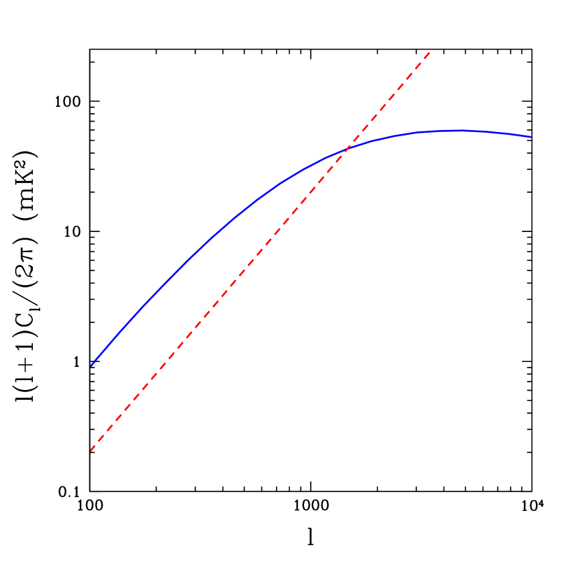
Figure 6: The noise power spectrum assumed in our analysis (red dashed line). Blue solid line - the 21cm signal at z=9.2 (140 MHz) with $\Delta\nu=1$ MHz.

5 Error forecast

Our goal is now to calculate the expected error in the 21cm power spectrum, taking into account the experimental noise and foreground contamination. Given a set of measurements $\{y\}$, the information of how well we can measure a set of parameters $\{p\}$, is contained in the Fisher information matrix (Kendall & Stuart, 1979)

$$F_{ij}=\left\langle{\partial^{2}\log{\cal L}\over\partial p_{i}\partial p_{j}}\right\rangle,$$ (30)

where ${\cal L}(y,p)$ is the likelihood of parameters $\{p\}$ given observations $\{y\}$ and the matrix is to be evaluated at the true values of the parameters $\{p\}$. For now, we consider these parameters to be the 21cm auto power spectra binned in multipole and frequency space plus the foreground model parameters. The Cramér-Rao inequality states that $(F^{-1})_{ij}$ is the smallest variance that any unbiased estimator of the parameters can have (see Tegmark et al. 1997 for a review).

For an interferometer, we can take the set of measurements $\{y\}$ to be the measured visibilities, $V({\bf u},\nu)$. Assuming all fluctuations are Gaussian with zero mean ($\langle y\rangle=0$) the Likelihood is entirely specified by the covariance matrix ${\bf C}\equiv\langle yy^{t}\rangle=\langle V({\bf u},\nu)V^{*}({\bf u}^{\prime},\nu^{\prime})\rangle$. Note that the brightness temperature is not exactly Gaussian (see Furlanetto et al. 2004a). In order to obtain large values of the temperature we need regions with large densities, but these are typically ionized giving $T_{21}=0$, so that the Gaussian distribution will be cut for large values. However, as long as we are probing scales much larger than the effective patch size, the signal will be an average over many bubbles and we expect the Gaussian assumption to be a good approximation for the Fisher matrix analysis. We also make the approximation that the foreground fluctuations are Gaussian distributed. While this assumption holds true for high-redshift contributions, such as free-free point sources, foregrounds such as synchrotron emission within the Galaxy are highly non-Gaussian over large areas on the sky. Our Gaussian assumption is then expected to underestimate the effect of foregrounds at large angular scales corresponding to tens of degrees. However, here we will consider measurements of 21 cm fluctuations at a degree scale and below so that the Gaussian approximation is expected to be a reasonable one.

The covariance matrix can be quite complex due to the cross-correlations between different ${\bf u}$. To proceed further we assumed a bin size in $l=2\pi|{\bf u}|$ space such that this cross-correlation is negligible. The matrix ${\bf C}$ will then become block diagonal, making the Fisher matrix analysis more straightforward. As discussed in the previous section, it will be necessary to create an effective beam such that the correlation length is constant across frequency. We choose $\Delta l=100$ which, for the experimental setup described above (§4) makes the values almost uncorrelated among different $l$. The number of independent measurements at a given $l=2\pi|{\bf u}|$ is then $N_{l}={\pi lt_{total}\over\Delta lt_{0}}$.

We will proceed the analysis making reference to the angular power spectrum instead of the power in the visibilities, knowing that the two can be related through equation (23). The covariance at a given $l$ between two frequency bins $(i,j)$ is:

$${\bf C}^{l}_{ij}=C^{f}_{l}(\nu_{i},\nu_{j})+C^{s}_{l}(\nu_{i},\nu_{j})+C_{l}^{N}(\nu_{i},\nu_{j})\delta_{ij}\,.$$ (31)

The corresponding Fisher matrix is then,

$${\cal F}_{ab}\approx\sum_{l}{{N_{l}\over 2}Tr\left[({\bf C}^{l})^{-1}{\partial{\bf C}^{l}\over\partial p_{a}}({\bf C}^{l})^{-1}{\partial{\bf C}^{l}\over\partial p_{b}}\right]},$$ (32)

where $\{p_{a},\,p_{b}\}$ are the parameters we wish to estimate.

5.1 Power Spectrum

In this section we investigate how well we will be able to measure the 21cm power spectrum. To better understand the impact our foreground models will have on foreground removal, we start by just considering one type of foreground (point sources) and assume that all its statistical properties are known. Our parameters are then: $p_{a}=C_{l}^{21}(\nu_{a},\nu_{a})$ and we assume that the correlation of this signal across frequency, e. g. ${C_{l}^{s}(\nu_{a},\nu_{b})/\sqrt{C_{l}^{s}(\nu_{a},\nu_{a})C_{l}^{s}(\nu_{b},\nu_{b})}}$, is known from theory.

We can calculate an approximate expression for the expected error in $C_{l}^{21}(\nu_{i},\nu_{i})$ which will make it easier to understand the results from the Fisher matrix analysis. If the foregrounds were perfectly correlated across frequencies ($a^{f}_{lm}(\nu_{2})=\gamma a^{f}_{lm}(\nu_{1})$) and the signal uncorrelated, then clearly by subtracting the two maps ($a_{lm}(\nu_{2})-\gamma a_{lm}(\nu_{1})$) the foregrounds would be completely removed. A decrease in the foreground correlation translates into fluctuations in $\gamma$ so that the foreground subtraction is not as effective. Using only two frequency bins, the corresponding error of the 21cm power spectrum is then (see Zaldarriaga et al. 2004)

$$(\Delta C^{21}_{l})^{2}\approx{2\over 2l+1}\left[C^{s}_{l}+C^{N}_{l}+C^{f}_{l}(1-I)\right]^{2},$$ (33)

where $I$ is the correlation coefficient and we have assumed the signal power spectrum to be the same in both frequencies. Cleaning in this case is very effective, with foreground contamination down by $C^{f}_{l}(1-I)$.

We want to reconstruct the signal power spectrum as a function of frequency and so now drop this assumption of frequency independence. Without this assumption, two channels are now only sufficient for constraining a linear combination of the signal power spectra, not the signal power spectra themselves. However, with $N$ channels, $N(N-1)/2$ different foreground-cleaned maps can be made (one for each pair of maps) which is more than the $N$ signal power spectra to be determined if $N>2$, making the reconstruction possible. The more channels, the more pairs of maps and the more estimates of the power spectra we have. If all of these map pairs had similar, and independent, information about the signal power spectra, then we would expect the errors on each power spectrum to improve as $\sim\sqrt{(N-1)/2}$. Actually, the errors are correlated, and the difference maps made from larger frequency separations have greater residual foreground contamination, so the improvement is slower than $\sqrt{(N-1)/2}$ if one increases $N$ by increasing the frequency coverage.

The growing decoherence of the foregrounds over large frequencies limits how well an expanded frequency coverage can improve the reconstruction. Likewise, the coherence of the signal over very small frequency separations limits how well a refined binning can improve the reconstruction. With a fine enough binning, moving to finer binning no longer increases the effective number of independent frequency bins. Figure 7 shows the expected foreground and signal correlations across frequency. Although, as expected, the foreground is much more strongly correlated than the signal, there is a non-negligible signal correlation. The moderate correlation strength for frequency separations equal to the bandwidth (about 30%) suggests that there will be some improvement in reconstruction from making bands finer than 1 MHz, but that 1 MHz is near the point of highly diminished returns, at least for $l\lesssim 1000$. Binning an order of magnitude more finely than our nominal 1 MHz bins would also result in the added challenge of having to take into account redshift distortions due to the peculiar velocities of the neutral gas. With 1 MHz binning the redshift distortions are negligible.

Figure 7: Expected frequency cross-correlations for foregrounds (top) and signal (bottom) at $l=1000$ ($\Delta\nu=1$ MHz).

In Figure 8 we show the expected error in the 21 cm power spectrum taking into account the experimental setup described above and only assuming point source contamination. We used the point source parameters from Table 1. The red thin lines use information from 40 frequency bins (from 120MHz to 160MHz) while the green thick curves only use ten bins (from 135MHz to 145MHz). The larger the number of bins, the smaller is the recovered error, as expected from the above discussion. Since foreground subtraction is difficult at frequency separations less than 1MHz, the best way to improve on this result will be to expand the frequency range, although this can be problematic due to the man-made electromagnetic interference. Note however that the recovered error using our fiducial point source model (thin solid line) is already quite close to the ideal situation with no foreground contamination (dotted line). Assuming perfectly correlated foregrounds (short-dashed line), the errors come very close to the no foreground case; they would be identical were it not for the signal correlation.

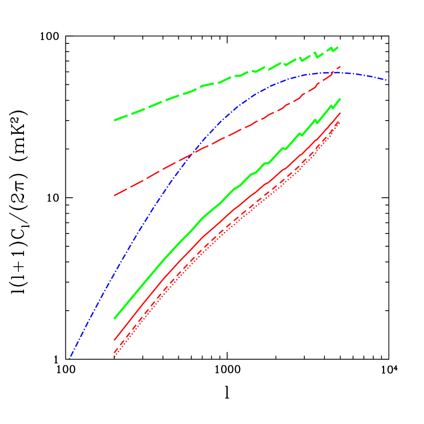
Figure 8: Expected error on the power spectrum at 140MHz (1MHz bin size), assuming only point sources contamination (no free parameters). Blued dot-dashed line - the 21cm signal. All other curves show the recovered errors for different assumptions about the point source model, using 40 frequency bins (thin red lines) and 10 bins (thick green lines). Dotted line - error with no foregrounds. Solid curve - assuming a Gaussian correlation across frequency. Short-dashed curve - point sources fully correlated. Long-dashed curve - assuming a constant correlation. This constant correlation case uses $I\sim 1-3\times 10^{-5}$ (the value of the Gaussian at 1MHz separations).

Comparing the solid and long-dashed curves, we also see that the Gaussian form of the foreground correlations (e.g. equation 15) allows the foreground removal to be more efficient than in the constant correlation case. This is an important result that we will explore in the next section.

Note also that we are presenting this result for a bin at the middle of the frequency range. Figure 9 shows the power spectrum and its errors at $l=1000$, versus the frequency, again assuming only point source contamination. As we move closer to the end of the frequency interval, the error increases, since the number of neighboring channels decreases (also, for lower frequencies, the foreground contribution is typically larger). However, using the full frequency range still provides great statistical power when distinguishing between different reionization models as we will see later in §6.

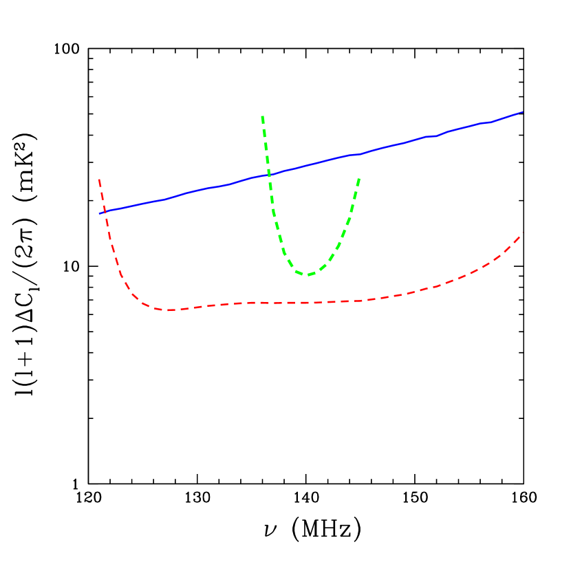
Figure 9: The 21cm signal at $l=1000$ as a function of frequency (blue solid curve) and the corresponding errors. We are assuming only point source contamination (parameters from Table 1). Red thin dashed line shows the recovered errors using 40 frequency bins. Green thick dashed line shows the same for 10 bins.

5.2 Dependence on assumptions about frequency coherence and its functional form

In general, the more coherent a foreground is, the easier it will be to remove it. This can be seen in Figure 10 where we plot the recovered error for the power spectrum at $l=1000$ as a function of the correlation length, $\xi$ (solid curve). As above, we are using a Gaussian form for the correlation function.

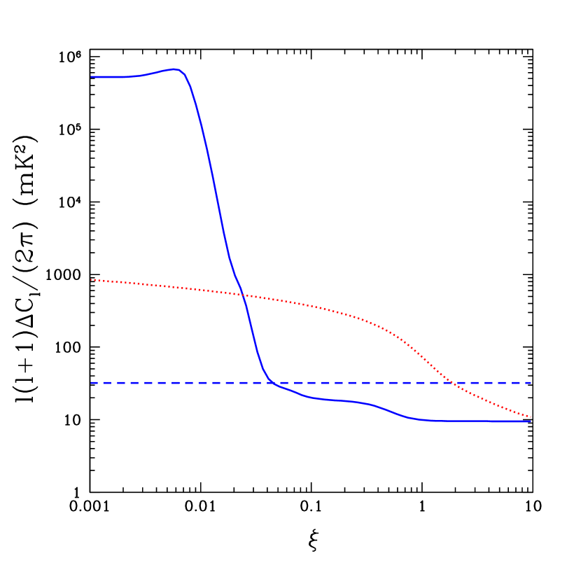
Figure 10: Dependence of the expected error on the foreground correlation length (at z=9.2 and $l=1000$) using a Gaussian correlation function (blue solid line). Red dotted line shows the same for the thick solid curve in Figure 11 (e.g. the worst case scenario). Blue dashed line shows the signal.

As expected, the situation gets worse as we move from the ideal case of perfect foreground coherence (large $\xi$) to completely incoherent foregrounds (small $\xi$). In the latter case, the foregrounds simply act as a huge noise component. Foreground removal is shown to be effective as long as $\xi\gtrsim 0.1$ which, if the point sources have a Poisson distribution, would translate into $\Delta\alpha\lesssim 10$. If the point source fluctuation power is mainly from correlations and we conservatively set $\sigma_{\alpha}=\Delta\alpha$, then $\xi\gtrsim 0.1$ once again translates into $\Delta\alpha\lesssim 10$. We see that our extrapolations based on data with brighter point sources would have to be very far off in order for the uncertainty in the 21cm fluctuation power spectrum to be significantly increased.

The shape of the correlation function (equation 14) also has a very important impact on how well foregrounds can be removed. In fact we have already seen in Figure 8 that the (unphysical) assumption of constant cross-frequency correlations results in larger errors, even though the foreground correlations between different frequencies are always larger than in the Gaussian case (a similar effect, albeit in a different scenario, was already noticed in Tegmark et al. 2000). Since the coherence function, $I(\nu_{1},\nu_{2})$, has not yet had its shape accurately measured, we decided to repeat the Fisher analysis for a variety of such functions. We can rewrite the coherence function (equation 15) as $I(\nu_{1},\nu_{2})=f\left[\log(\nu_{1}/\nu_{2})/\xi\right]$, where, for our fiducial model, $f(x)=e^{-x^{2}/2}$. Although this function should behave like a parabola near the origin ( equation 16), with $f(0)=1$, $f^{\prime}(0)=0$ and $f^{\prime\prime}(0)=-1$ (Tegmark, 1998), it does not have to necessarily be a Gaussian, so that we also considered functions of the form

$$f(x)=\left(1+{x^{2}\over 2n}\right)^{-n}.$$ (34)

We recover the Gaussian case for $n=\infty$ (actually, for the typical range of values in $x$ we are considering, $n=10$ is already a good approximation to a Gaussian).

Figure 11 shows the foreground correlations for several values of $n$ (decreasing $n$ increases the values at the tails of the distribution).

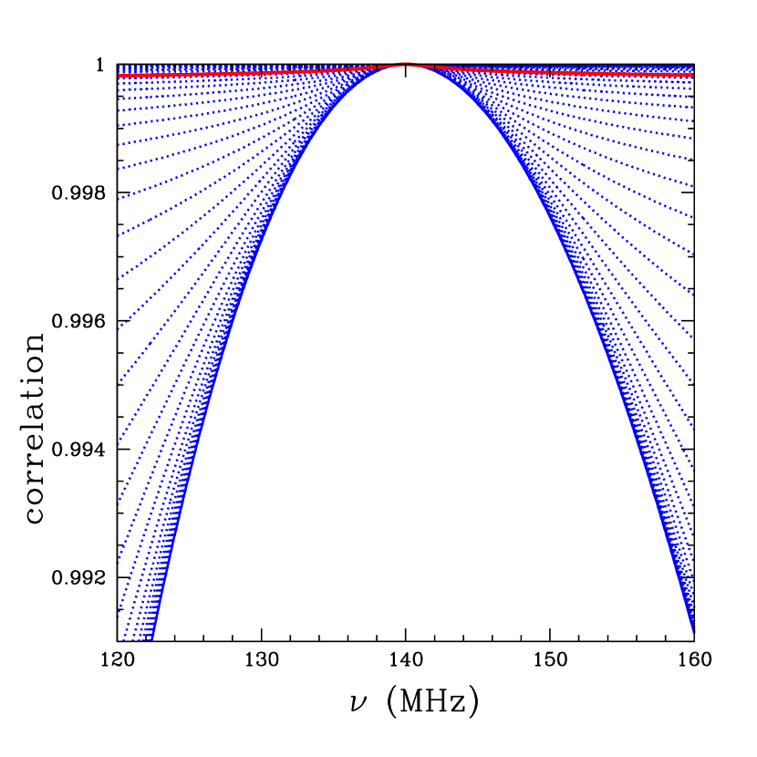
Figure 11: Several functions for the foreground correlations of the type: $(1+x^{2}/2/n)^{-n}$ with $x=log(\nu_{1}/\nu_{2})/\xi$. Gaussian: n$\rightarrow\infty$ ($e^{-x^{2}/2}$). Red thick solid line gives the largest error and is very similar to the constant case with a correlation at 1MHz separations identical to the Gaussian case.

In Figure 12 we show the recovered error in the power spectrum at $l=1000$ using the above functions. In this case we are only using 10 bins of 1 MHz each, centered around 140MHz (solid line).

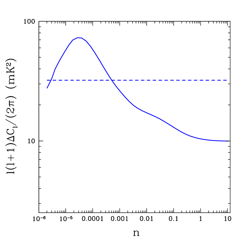
Figure 12: The recovered error at $l=1000$ and $\nu=140$ MHz, assuming point sources contamination and using the correlation functions from figure 11 (blue solid line). Dashed line shows the signal.

Notice that, although all the functions have larger cross-frequency correlations than the Gaussian case, foreground removal is always worse than with the Gaussian form (large $n$). The behavior of $f(x)$ away from the origin is quite important. As $n$ decreases, the second derivative of $f(x)$ for $x\neq 0$ also decreases, so that the function approaches the linear (and almost constant) case. This translates into an increase in the recovered error which peaks at $n\sim 3\times 10^{-5}$. At this point, the correlation for separations of 1MHz (the bin size we have been using) is still approximately the same as in the Gaussian case. As $n$ decreases further, the frequency correlations increase (even at 1MHz separations) and the function converges to 1 everywhere (foregrounds fully correlated), so that the recovered error decreases again. Clearly, for foreground removal to be effective in the worst case scenario function, we need the correlation length to be larger. Figure 10 also shows the recovered error as a function of correlation length for this worst case value of $n$ (red dotted lines). In order to measure the signal we need $\xi>1$ which implies $\Delta\alpha<1$.

5.3 Simultaneous estimation of foregrounds and the 21cm power spectrum

Up to now we have assumed that all the statistical properties of the foregrounds are perfectly known. In fact, we hope to learn a lot about the spatial and frequency dependence of foregrounds from experiments set to measure the 21cm signal. Information about the spectral index of point sources at the frequencies of interest, for instance, can be obtained by using the large baselines available with the interferometer experiments. This combined with observational data on foregrounds at frequencies slightly higher than 1421 MHz should provide us with an improved foreground model prior to the data analysis. However, because of the huge foreground amplitude compared to the 21cm signal, even very small variations to the assumed model might be confused with the signal and bias the estimation. In particular, as we have seen above, a good knowledge of the foreground frequency coherence structure in the range of interest will be crucial to the analysis. Therefore, we will now allow for free parameters in our foreground model and consider the case in which these parameters, together with the 21cm power spectra are simultaneously estimated from the data. Our foreground model is as given in equations  13 with

$$I_{l}(\nu_{1},\nu_{2})=\left(1+{\log^{2}{(\nu_{1}/\nu_{2})}\over 2n\xi^{2}}\right)^{-n}.$$ (35)

The parameters to estimate are $p=\{A,\beta,\bar{\alpha},\xi,\log(n)\}$ for each of the four foregrounds we are considering (point sources, Galactic synchrotron, extragalactic free-free and Galactic free-free emission) and $p_{a}=C_{l}^{21}(\nu_{a},\nu_{a})$. We use 49 bins in $l$ space at each frequency (from $l=200$ to 5000 with $\Delta l=100$) and 40 bins of 1MHz from 120MHz to 160MHz ($z=7.9$ to $z=10.8$) giving a total of 1980 parameters (20 parameters for the foregrounds plus 1960 for $C_{l}^{21}(\nu_{a},\nu_{a})$). Each bin in $l$ space has $N_{l}={\pi lt_{total}\over\Delta lt_{0}}$ independent $a_{lm}$ measurements so that there will be a total of 642605 input data points in the form of $a_{lm}$ values. We show in Figure 13 the estimated error on the power spectrum for the frequency bin of 140MHz from our full calculation.

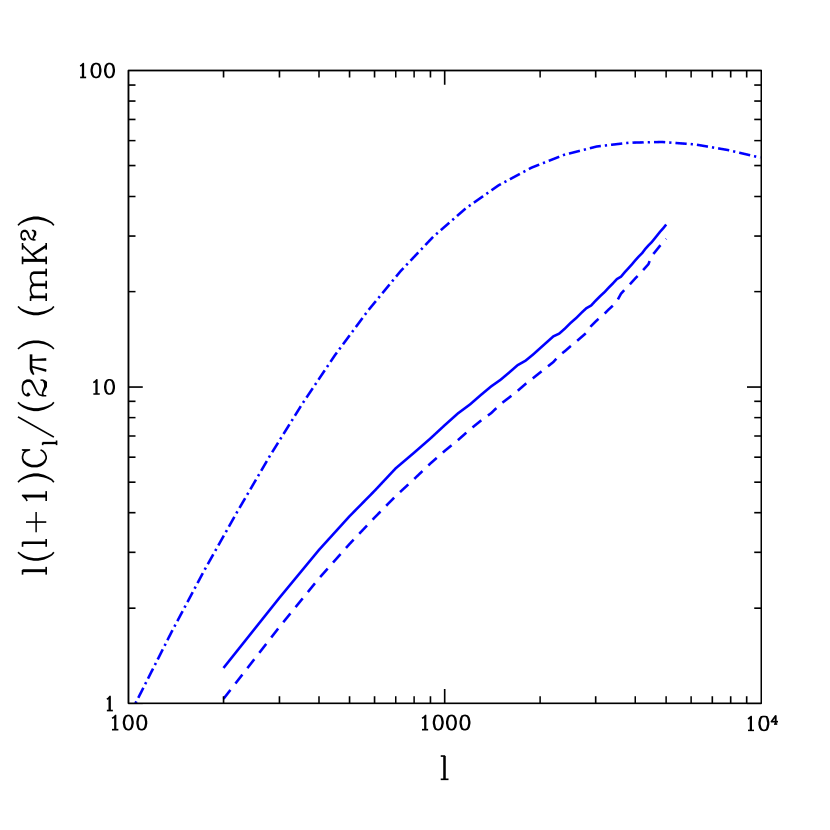
Figure 13: Expected error on the power spectrum at 140MHz, when including point sources, Galactic synchrotron, extragalactic free-free and Galactic free-free (blue solid line). Dashed line gives the case with no foregrounds. Dot-dashed line shows the signal.

Using these 40 frequency bins, the foreground removal is quite efficient with the errors only showing a small foreground contamination. Note however that these errors will increase as we move toward the limits of the frequency range, as shown earlier in Figure 9.

6 Constraining the reionization model

Given a model of the perturbations in the ionization fraction we can ask how well one can constrain the corresponding free parameters. Typically, the ionization fraction power spectrum can be divided into two regions. First, on large enough scales, we expect the fraction of ionized material to follow the number of halos above a certain mass. The power spectrum will then be proportional to the matter density, with a bias factor that is expected to be larger than one. Second, as the scales approach the ionized bubble size, the power should be smoothed out since there are no fluctuations from inside the bubbles (this small scale cutoff might be quite extended if there is a wide distribution of bubble sizes). The transition from one region to the other is model dependent. We are probing redshifts from $z\sim 8$ to $z\sim 11$ up to $l\sim 1000$ corresponding to scales $x\gtrsim 9{\rm Mpc}$ which we expect to be larger than the typical bubble size in our model. We therefore model the ionization fraction power spectrum as

$$P_{\delta_{x}\delta_{x}}(k,z)\sim b^{2}(z)P_{\delta\delta}(k,z)$$ (36)

and choose our free parameter to be $b_{x}\equiv\bar{x}_{e}b(z)$. For large bias ($b(z)$), the main contribution to equation 10 is then $b_{x}^{2}(z)P_{\delta\delta}(k,z)$. We have therefore a total of 60 parameters in our model (one $b_{x}$ for each of the 40 frequency bins plus 20 foreground parameters). Figure 14 shows the expected error from our full calculation. For comparison we also plot the expected $b_{x}$ from two other reionization models with the same optical depth (see Figures 3 and 4). The recovered error is only at a few percent level so that, by measuring this parameter, it should be possible to distinguish between different reionization histories.

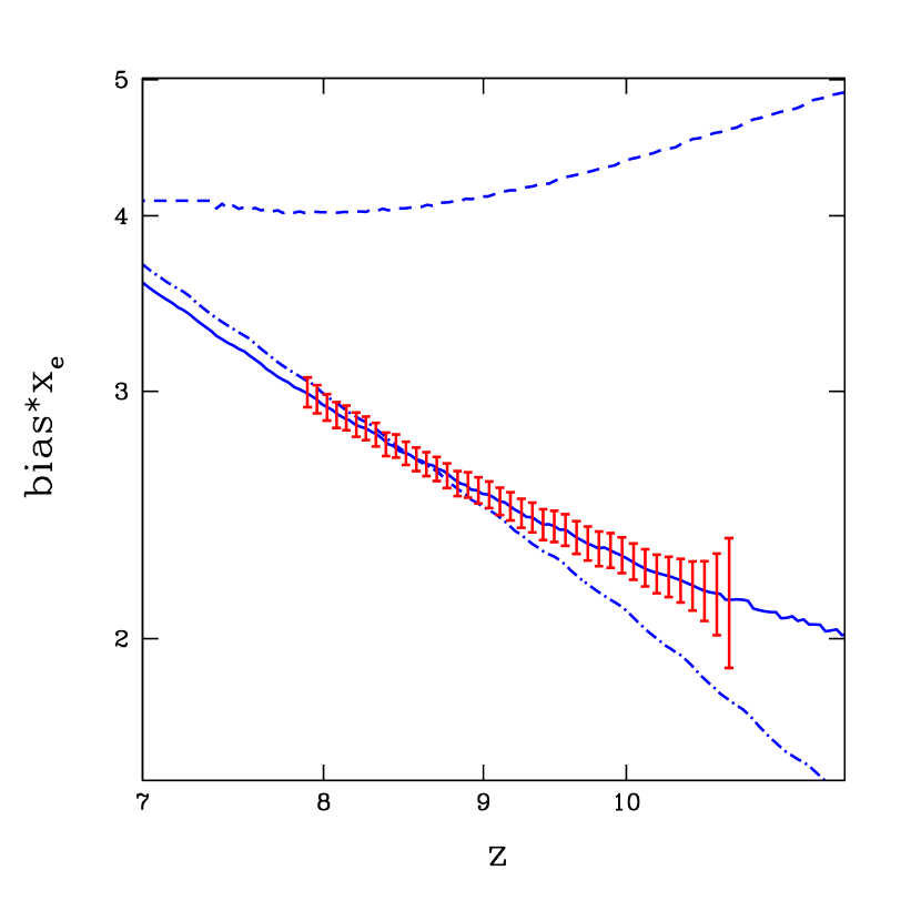
Figure 14: Expected error on the product of the bias times the ionization fraction. Models are the same as in Figures 3 and 4.

7 Summary

The measurement of the 21cm radiation from neutral hydrogen at high redshifts will provide unprecedent information about the epoch of reionization. Unfortunately this signal has a huge foreground contamination, several orders of magnitude above the 21cm fluctuations (Oh & Mack, 2003), making its detection a real challenge. In this paper we have presented a detailed study of the foregrounds and the manner in which they will affect the measurement of the 21cm perturbations. We consider four types of foregrounds: diffuse Galactic synchrotron emission at low radio frequencies, Galactic free-free, extragalactic free-free emission and extragalactic point sources. We analyzed both the case when the foreground power spectra are known and the case when their parameters must be determined from the 21cm data itself.

Our results are in general encouraging and show that we can achieve a high level of foreground cleaning even when using quite conservative choices for foreground models both in terms of foreground fluctuation amplitude and frequency coherence. The removal is aided by the large frequency cross-correlation for foreground signals, although their frequency dependence and spatial power spectra are also useful in distinguishing them from the 21 cm signal. The 21 cm signal correlations, between channels, also play an important role and basically set a minimum bandwidth to the frequency cleaning process in which foreground removal is still effective. We do not expect a binning finer than 1MHz to greatly improve the reconstruction. Also, as expected, foreground removal improves as we increase the number of frequency bins with fixed bin size. Using the full information from 40 bins of 1MHz each, it is possible to clean out the foreground signal almost completely from the background 21 cm signal.

The most crucial feature in the cleaning process is the foreground correlation structure. Concentrating on the point source contamination (which should be the most damaging foreground due to its smaller coherence), we see that the Gaussian correlation function provides the best results. In this case, limits on the spectral index variation are well above expected values from point source models. Even in the worst case scenario, when the function is nearly linear in $\log\left(\nu_{1}/\nu_{2}\right)$, foreground removal is still effective as long as the spectral index variations $\Delta\alpha\lesssim 1$, which is consistent with observations of point sources (Cohen et al., 2004). Our full statistical analysis allowed for variations in this correlation structure as well as the spectral index and shape of the angular power spectrum. Using a total of 40 bins from 120MHz to 160MHz and taking into account all the foregrounds, we calculated the expected errors for a total of 1975 parameters. The results show that foreground contamination will be minimal, allowing for a clear measurement of 21cm power spectra.

We also investigated how well one can constrain the reionization model, by making full use of the three dimensional nature of the data (both in frequency and angular dependence). Although a detailed parameterization of the reionization model incorporating all possible variations to the reionization history is difficult, we expect certain features to be robust. On scales larger than the patch size, for instance, the 21cm power spectra should follow the shape of the projected dark matter power spectrum. Our analysis has shown that the large-scale bias of the neutral Hydrogen gas distribution, with respect to the density field, can be determined with a high precision. This allows for an accurate distinction between certain reionization models, even if they have the same optical depth.

The technical requirements to measure the 21cm signal, although challenging, should be within reach by proposed experiments such as SKA, LOFAR and PAST. Instruments such as PAST can provide additional information related to foregrounds that can be used to optimize SKA/LOFAR surveys. The big question addressed in this paper was to quantitatively establish if foregrounds, when taken as a whole, would contaminate 21 cm measurements beyond repair. Our results show that the future for these experiments is quite promising: even fully taking into account the expected foregrounds, the 21 cm fluctuations can be measured well enough to be a powerful probe of reionization.

References

- Becker et al. (2001) Becker, R. H., Fan, X., White, R. L., Strauss, M. A., Narayanan, V. K., Lupton, R. H., Gunn, J. E., Annis, J., Bahcall, N. A., Brinkmann, J., Connolly, A. J., Csabai, I. ., Czarapata, P. C., Doi, M., Heckman, T. M., Hennessy, G. S., Ivezić, Ž., Knapp, G. R., Lamb, D. Q., McKay, T. A., Munn, J. A., Nash, T., Nichol, R., Pier, J. R., Richards, G. T., Schneider, D. P., Stoughton, C., Szalay, A. S., Thakar, A. R., & York, D. G. 2001, AJ, 122, 2850
- Bennett et al. (2003) Bennett, C. L., Halpern, M., Hinshaw, G., Jarosik, N., Kogut, A., Limon, M., Meyer, S. S., Page, L., Spergel, D. N., Tucker, G. S., Wollack, E., Wright, E. L., Barnes, C., Greason, M. R., Hill, R. S., Komatsu, E., Nolta, M. R., Odegard, N., Peirs, H. V., Verde, L., & Weiland, J. L. 2003, ArXiv Astrophysics e-prints, 2207
- Benson et al. (2001) Benson, A. J., Nusser, A., Sugiyama, N., & Lacey, C. G. 2001, MNRAS, 320, 153
- Bharadwaj & Ali (2005) Bharadwaj, S., & Ali, S. S. 2005, MNRAS, 356, 1519
- Cen (2003) Cen, R. 2003, ApJ, 591, 12
- Cen & McDonald (2002) Cen, R., & McDonald, P. 2002, ApJ, 570, 457
- Chen et al. (2003) Chen, X., Cooray, A., Yoshida, N., & Sugiyama, N. 2003, MNRAS, 346, L31
- Chen & Miralda-Escudé (2004) Chen, X., & Miralda-Escudé, J. 2004, ApJ, 602, 1
- Cohen et al. (2004) Cohen, A. S., Röttgering, H. J. A., Jarvis, M. J., Kassim, N. E., & Lazio, T. J. W. 2004, ApJS, 150, 417
- Condon et al. (1998) Condon, J. J., Cotton, W. D., Greisen, E. W., Yin, Q. F., Perley, R. A., Taylor, G. B., & Broderick, J. J. 1998, AJ, 115, 1693
- Cooray & Furlanetto (2004) Cooray, A., & Furlanetto, S. R. 2004, ApJ, 606, L5
- Cooray & Sheth (2002) Cooray, A., & Sheth, R. 2002, Phys. Rep., 372, 1
- de Oliveira-Costa et al. (1998) de Oliveira-Costa, A., Tegmark, M., Page, L. A., & Boughn, S. P. 1998, ApJ, 509, L9
- Di Matteo et al. (2004) Di Matteo, T., Ciardi, B., & Miniati, F. 2004, MNRAS, 355, 1053
- Di Matteo et al. (2002) Di Matteo, T., Perna, R., Abel, T., & Rees, M. J. 2002, ApJ, 564, 576
- Fan et al. (2002) Fan, X., Narayanan, V. K., Strauss, M. A., White, R. L., Becker, R. H., Pentericci, L., & Rix, H. 2002, AJ, 123, 1247
- Field (1959) Field, G. B. 1959, ApJ, 129, 525
- Furlanetto et al. (2004a) Furlanetto, S. R., Zaldarriaga, M., & Hernquist, L. 2004a, ApJ, 613, 16
- Furlanetto et al. (2004b) —. 2004b, ApJ, 613, 1
- Giavalisco et al. (1998) Giavalisco, M., Steidel, C. C., Adelberger, K. L., Dickinson, M. E., Pettini, M., & Kellogg, M. 1998, ApJ, 503, 543
- Gnedin (2000) Gnedin, N. Y. 2000, ApJ, 542, 535
- Gnedin (2004) —. 2004, ApJ, 610, 9
- Gnedin & Ostriker (1997) Gnedin, N. Y., & Ostriker, J. P. 1997, ApJ, 486, 581
- Gnedin & Shaver (2004) Gnedin, N. Y., & Shaver, P. A. 2004, ApJ, 608, 611
- Gunn & Peterson (1965) Gunn, J. E., & Peterson, B. A. 1965, ApJ, 142, 1633
- Haiman et al. (2001) Haiman, Z., Abel, T., & Madau, P. 2001, ApJ, 551, 599
- Haiman & Holder (2003) Haiman, Z., & Holder, G. P. 2003, ApJ, 595, 1
- Hales et al. (1988) Hales, S. E. G., Baldwin, J. E., & Warner, P. J. 1988, MNRAS, 234, 919
- Hernquist & Springel (2003) Hernquist, L., & Springel, V. 2003, MNRAS, 341, 1253
- Hu & Holder (2003) Hu, W., & Holder, G. P. 2003, Phys. Rev. D, 68, 023001
- Iliev et al. (2002) Iliev, I. T., Shapiro, P. R., Ferrara, A., & Martel, H. 2002, ApJ, 572, L123
- Kaiser (1992) Kaiser, N. 1992, ApJ, 388, 272
- Kaplinghat et al. (2003) Kaplinghat, M., Chu, M., Haiman, Z., Holder, G. P., Knox, L., & Skordis, C. 2003, ApJ, 583, 24
- Kendall & Stuart (1979) Kendall, M., & Stuart, A. 1979, The advanced theory of statistics. Vol.2: Inference and relationship (London: Griffin, 1979, 4th ed.)
- Kogut et al. (2003) Kogut, A., Spergel, D. N., Barnes, C., Bennett, C. L., Halpern, M., Hinshaw, G., Jarosik, N., Limon, M., Meyer, S. S., Page, L., Tucker, G. S., Wollack, E., & Wright, E. L. 2003, ApJS, 148, 161
- Kumar et al. (1995) Kumar, A., Padmanabhan, T., & Subramanian, K. 1995, MNRAS, 272, 544
- Laing et al. (1983) Laing, R. A., Riley, J. M., & Longair, M. S. 1983, MNRAS, 204, 151
- Lang (1999) Lang, K. R. 1999, Astrophysical formulae (Astrophysical formulae / K.R. Lang. New York : Springer, 1999. (Astronomy and astrophysics library,ISSN0941-7834))
- Madau et al. (1997) Madau, P., Meiksin, A., & Rees, M. J. 1997, ApJ, 475, 429
- Miralda-Escudé et al. (2000) Miralda-Escudé, J., Haehnelt, M., & Rees, M. J. 2000, ApJ, 530, 1
- Morales (2005) Morales, M. F. 2005, ApJ, 619, 678
- Morales & Hewitt (2003) Morales, M. F., & Hewitt, J. 2003, ArXiv Astrophysics e-prints, 2437
- Oh (1999) Oh, S. P. 1999, ApJ, 527, 16
- Oh & Mack (2003) Oh, S. P., & Mack, K. J. 2003, MNRAS, 346, 871
- Pen et al. (2004) Pen, U., Wu, X., & Peterson, J. B. 2004, ArXiv Astrophysics e-prints, 04083
- Platania et al. (1998) Platania, P., Bensadoun, M., Bersanelli, M., de Amici, G., Kogut, A., Levin, S., Maino, D., & Smoot, G. F. 1998, ApJ, 505, 473
- Rengelink et al. (1997) Rengelink, R. B., Tang, Y., de Bruyn, A. G., Miley, G. K., Bremer, M. N., Roettgering, H. J. A., & Bremer, M. A. R. 1997, A&AS, 124, 259
- Rohlfs & Wilson (2004) Rohlfs, K., & Wilson, T. L. 2004, Tools of radio astronomy (Tools of radio astronomy, 4th rev. and enl. ed., by K. Rohlfs and T.L. Wilson. Berlin: Springer, 2004)
- Santos et al. (2003a) Santos, M. G., Cooray, A., Haiman, Z., Knox, L., & Ma, C. 2003a, ApJ, 598, 756
- Santos et al. (2003b) Santos, M. G., Heavens, A., Balbi, A., Borrill, J., Ferreira, P. G., Hanany, S., Jaffe, A. H., Lee, A. T., Rabii, B., Richards, P. L., Smoot, G. F., Stompor, R., Winant, C. D., & Wu, J. H. P. 2003b, MNRAS, 341, 623
- Scott & Rees (1990) Scott, D., & Rees, M. J. 1990, MNRAS, 247, 510
- Shaver et al. (1999) Shaver, P. A., Windhorst, R. A., Madau, P., & de Bruyn, A. G. 1999, A&A, 345, 380
- Sokasian et al. (2003) Sokasian, A., Abel, T., Hernquist, L., & Springel, V. 2003, MNRAS, 344, 607
- Spergel et al. (2003) Spergel, D. N., Verde, L., Peiris, H. V., Komatsu, E., Nolta, M. R., Bennett, C. L., Halpern, M., Hinshaw, G., Jarosik, N., Kogut, A., Limon, M., Meyer, S. S., Page, L., Tucker, G. S., Weiland, J. L., Wollack, E., & Wright, E. L. 2003, ApJS, 148, 175
- Tegmark (1998) Tegmark, M. 1998, ApJ, 502, 1
- Tegmark et al. (2000) Tegmark, M., Eisenstein, D. J., Hu, W., & de Oliveira-Costa, A. 2000, ApJ, 530, 133
- Tegmark et al. (1997) Tegmark, M., Taylor, A. N., & Heavens, A. F. 1997, ApJ, 480, 22+
- Tozzi et al. (2000) Tozzi, P., Madau, P., Meiksin, A., & Rees, M. J. 2000, ApJ, 528, 597
- Venkatesan et al. (2001) Venkatesan, A., Giroux, M. L., & Shull, J. M. 2001, ApJ, 563, 1
- White et al. (1999) White, M., Carlstrom, J. E., Dragovan, M., & Holzapfel, W. L. 1999, ApJ, 514, 12
- Wyithe & Loeb (2003) Wyithe, J. S. B., & Loeb, A. 2003, ApJ, 588, L69
- Zaldarriaga (1997) Zaldarriaga, M. 1997, Phys. Rev. D, 55, 1822
- Zaldarriaga et al. (2004) Zaldarriaga, M., Furlanetto, S. R., & Hernquist, L. 2004, ApJ, 608, 622