The narrow-line quasar NAB 0205+024 observed with XMM-Newton

Abstract

The XMM-Newton observation of the narrow-line quasar NAB 0205+024 reveals three striking differences since it was last observed in the X-rays with $ASCA$. Firstly, the 2–10 keV power-law is notably steeper. Secondly, a hard X-ray flare is detected, very similar to that seen in I Zw 1. Thirdly, a strong and broad emission feature is detected with the bulk of its emission redward of 6.4 keV, and extending down to $\sim 5$ keV in the rest frame. The most likely explanation for the broad feature is neutral iron emission emitted from a narrow annulus of an accretion disc close to the black hole. The hard X-ray flare could be the mechanism which illuminates this region of the disc, allowing for the emission line to be detected. The combination of effects can be understood in terms of the ‘thundercloud’ model proposed by Merloni & Fabian.

1 Introduction

Narrow-line Seyfert 1 galaxies (NLS1) offer an extreme view of the Seyfert 1 phenomenon. For example, these objects show:

• The narrowest permitted optical lines, strongest optical Fe ii emission, and weakest [O iii] emission (e.g. Osterbrock & Pogge 1985; Boroson & Green 1992; Grupe 2004).

• Strong soft X-ray excesses (e.g. Boller, Brandt & Fink 1996; Leighly 1999a; Vaughan et al. 1999) above a relatively steep hard power-law (e.g. Brandt, Mathur & Elvis 1999);

• Large-amplitude X-ray variations on hourly time scales (e.g. Boller, Brandt & Fink 1996; Leighly 1999b).

• Weak or negligible optical variability (e.g. Klimek, Gaskell & Hedrick 2004).

Many of the properties can be explained in terms of a high accretion rate and relatively low-mass black hole (e.g. Sulentic et al. 2000; Boroson 2002; Grupe 2004). These characteristics are not exclusive to lower-luminosity AGN (i.e. Seyfert 1s), but are also seen in some quasar-type objects. The most famous of these narrow-line quasars is the prototype I Zw 1, but the class also includes members such as PHL 1092, E 1346+266, IRAS 13349+2438, and the Neta A. Bahcall object NAB 0205+024 (Bahcall, Bahcall & Schmidt 1973).

NAB 0205+024 (Mrk 586; $z=0.155$) has been the focus of previous X-ray studies with $ASCA$ (e.g. Fiore et al. 1998), and $ROSAT$ (Fiore et al. 1994). The strong soft excess and rapid variability (by factors of two on time scales of hours) have made it an important object to study the nature of NLS1 behaviour in luminous narrow-line quasars.

In this paper we discuss the X-ray analysis of NAB 0205+024 as observed with XMM-Newton. The X-ray brightness of NAB 0205+024 (compared to other similar objects) affords us the opportunity to study the NLS1 phenomenon in a quasar with relatively high signal-to-noise.

2 Observations and data reduction

NAB 0205+024 was observed with XMM-Newton (Jansen et al. 2001) for $50$ ks on 2002 July 23 (revolution 0480). During this time the EPIC pn (Strüder et al. 2001) and MOS (MOS1 and MOS2; Turner et al. 2001) cameras, as well as the Optical Monitor (OM; Mason et al. 2001) and the Reflection Grating Spectrometers (RGS1 and RGS2; den Herder et al. 2001) collected data. The EPIC pn and MOS2 cameras were operated in full-frame mode and utilised the thin filter. The MOS1 camera was operated in timing mode, and the data will not be included in the current analysis.

The Observation Data Files (ODFs) were processed to produce calibrated event lists using the XMM-Newton Science Analysis System (SAS v6.0.0). Unwanted hot, dead, or flickering pixels were removed as were events due to electronic noise. Event energies were corrected for charge-transfer losses, and EPIC response matrices were generated using the SAS tasks ARFGEN and RMFGEN. Light curves were extracted from these event lists to search for periods of high background flaring. High-energy background flaring was substantial. The total good exposure times selected for the pn and MOS2 were 20388 s and 31545 s, respectively. The source plus background photons were extracted from a circular region with a radius of 35^′′, and the background was selected from an off-source region with a radius of 50^′′ and appropriately scaled to the source region. Single and double events were selected for the pn detector, and single-quadruple events were selected for the MOS2. Pile-up effects were determined to be negligible in the time-averaged data. However, there was mild pile-up during a $\sim 4{\rm\thinspace ks}$ period when the source flux increased by $50\%$ (Sect. 4). As a consistency check the inner $5{\hbox{${}^{\prime\prime}$}}$ of the source extraction region was removed, thus correcting the pile-up effect during the flare. The step proved to be unnecessary, as it had little effect on the spectral variability results (Sect. 4.2). The total numbers of source plus background counts collected in the 0.3–10 keV range by the pn and MOS2 instruments were 68372 and 29354, respectively. The total numbers of counts collected from the scaled background region were 1187 for the pn, and 1132 for the MOS2. The XMM-Newton observation provides a substantial improvement in spectral quality over the 51.8 ks $ASCA$-SIS exposure (118.6 ks duration) in which $\approx 18130$ counts were collected (Leighly 1999b).

The RGS were operated in standard Spectro+Q mode. The first-order RGS spectra were extracted using the SAS task RGSPROC, and the response matrices were generated using RGSRMFGEN. The total exposure times utilised for the analysis were 46078 s and 44717 s for the RGS1 and RGS2, respectively. The total number of source counts in the 0.35–1.5 keV range were approximately 4915 (RGS1) and 4708 (RGS2).

The OM was operated in imaging mode for the entire observation. In total, thirty-one 1000 s images were taken in three filters: 21 in $U$ ($3000-3900{\rm\thinspace\AA}$), and 5 in both $B$ ($3900-4900{\rm\thinspace\AA}$) and $UVW2$ ($1800-2250{\rm\thinspace\AA}$). The average apparent magnitude in each filter was $U=14.614\pm 0.002$, $B=15.701\pm 0.004$, and $UVW2=14.126\pm 0.011$.

3 Spectral analysis

Each of the EPIC spectra was compared to the respective background spectrum to determine the energy range in which the source was reasonably detected above the background. The source was detected above the background up to an observed energy of $\sim 10$ keV, and $\sim$ 7 keV in the pn and MOS2 data, respectively. The MOS data were ignored below 0.5 keV due to the uncertainties in the low-energy redistribution characteristics of the cameras (Kirsch 2003). Therefore, the pn data between 0.3–10 keV and the MOS2 data between 0.5–7 keV were utilised during the spectral fitting, but the residuals from each instrument were examined separately to judge any inconsistency. In addition the RGS data between 0.35–1.5 keV were also examined.

The source spectra were grouped such that each bin contained at least 20 counts. Spectral fitting was performed using XSPEC v11.3.0 (Arnaud 1996). Fit parameters are reported in the rest-frame of the object, although the figures remain in the observed-frame. The quoted errors on the model parameters correspond to a 90% confidence level for one interesting parameter (i.e. a $\Delta\chi^{2}$ = 2.7 criterion). Luminosities were derived assuming isotropic emission. The Galactic column density toward NAB 0205+024 is ${N_{\rm H}}=3.51\times 10^{20}\hbox{${\rm\thinspace cm}^{-2}\,$}$ (Dickey & Lockman 1990). A value for the Hubble constant of $H_{0}$=$\rm 70\ km\ s^{-1}\ Mpc^{-1}$ and a standard cosmology with $\Omega_{M}$ = 0.3 and $\Omega_{\Lambda}$ = 0.7 was adopted.

3.1 The broad-band X-ray continuum

A single power-law with Galactic absorption was a poor fit to the EPIC data between 0.3–10 keV ($\chi^{2}=1937.7/738~{}dof$). The higher statistics in the low-energy range dominate the fit resulting in large residuals at higher energies which demonstrates the need for multiple continuum components. Fitting only the EPIC data above 2 keV with an absorbed power-law resulted in a good fit ($\chi^{2}=272.4/302~{}dof$) and demonstrated agreement in the photon indices measured by each instrument ($\Gamma_{pn}=2.26\pm 0.07$ and $\Gamma_{MOS2}=2.20\pm 0.10$). Extrapolating this model to lower energies revealed a strong soft excess above the power-law continuum (Figure 1).

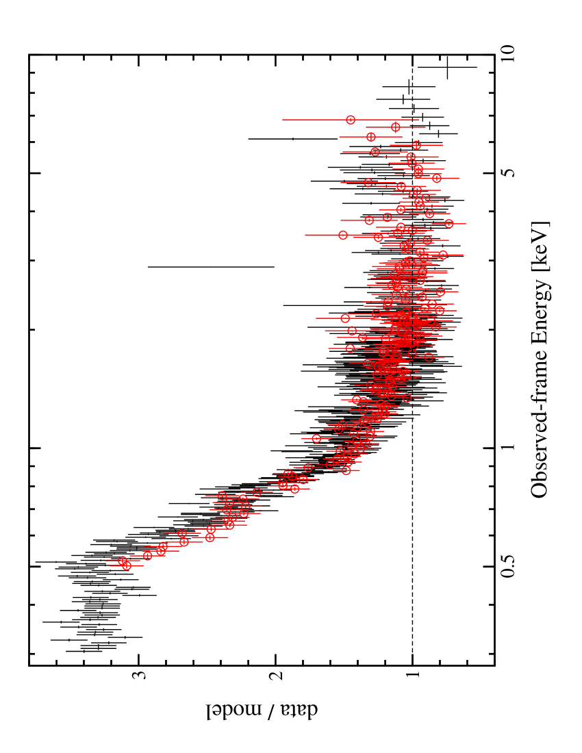
Figure 1: The ratio (data/model) resulting from fitting an absorbed power-law ($\Gamma_{pn}=2.26\pm 0.07$ and $\Gamma_{MOS2}=2.20\pm 0.10$) to the 2–10 keV EPIC data and extrapolating to lower energies. The black crosses and red open circles are the pn and MOS2 residuals, respectively. The apparently “wild” single data point at $E\approx 3$ keV is less than $3\sigma$ above the ratio, and probably is just a statistical fluctuation. The data have been binned for display purposes.

To investigate the nature of the continuum emission additional components were included in the basic power-law fit to model the soft excess. The data from each instrument were modelled separately in order to compare the results. In the case of the RGS, the high-energy model component (i.e. the power-law) was kept fixed to the pn values.

To fit the broad-band continuum a number of models were used including (i) a blackbody plus power-law, (ii) a double power-law and, (iii) a broken power-law. The addition of a second continuum component was a substantial improvement to the initial power-law fit; the best fit was obtained with model (i) (Figure 2). In this case the blackbody temperature was $kT\approx 120$ eV, and the intrinsic absorption was negligible. The 0.3–10 keV flux and luminosity, corrected for Galactic absorption, were $8.6\times 10^{-12}\hbox{${\rm\thinspace erg}{\rm\thinspace cm}^{-2}{\rm\thinspace s}^{-1}\,$}$ and $6.2\times 10^{44}\hbox{${\rm\thinspace erg}{\rm\thinspace s}^{-1}\,$}$, respectively. The 2–10 keV luminosity was $1.1\times 10^{44}\hbox{${\rm\thinspace erg}{\rm\thinspace s}^{-1}\,$}$. In Table LABEL:tab:cont the model parameters for each fit are given.

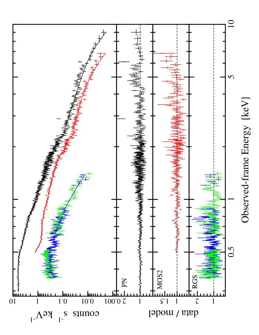
Figure 2: The best-fit continuum model (blackbody plus power-law) fitted to the XMM-Newton data. In the top panel the fit and data are shown for the pn (upper curve; black), MOS2 (middle curve; red), and RGS (lower curve; blue and green). In the remaining panels the fit residuals (data/model) are shown for each instrument.

Table 1: X-ray continuum models. The data from each EPIC instrument were modelled separately, but the RGS1 and RGS2 data were fitted together. The superscript $f$ marks the RGS parameters which are fixed to the best-fit pn values. The three continuum models, shown in column (1), are: (i) blackbody plus power-law, (ii) double power-law, and (iii) broken power-law. In column (2) we indicate the instrument used to collect the data, and in column (3) the fit quality ($\chi^{2}_{\nu}$) is given. Column (4) gives the measured intrinsic cold absorption. Column (5) is the temperature of the blackbody component. Columns (6) and (7) are the photon indices of the power-law components (two power-laws are required for models (ii) and (iii)). Column (8) is the energy at which the photon index changes between $\Gamma_{1}$ and $\Gamma_{2}$ in model (iii). All models have been modified by line-of-sight Galactic absorption (3.51 $\times$ 10²⁰ cm^-2).

(1)	(2)	(3)	(4)	(5)	(6)	(7)	(8)
Continuum	Instrument	$\chi^{2}_{\nu}$	${N_{\rm H}}$	$kT$	$\Gamma_{1}$	$\Gamma_{2}$	$E_{brk}$
Model		(dof)	(10${}^{20}\hbox{${\rm\thinspace cm}^{-2}\,$}$)	(eV)			(keV)
(i)	pn	1.04 (523)	$<0.3$	$121\pm 2$	$2.41\pm 0.04$
	MOS2	0.88 (209)	$<1.4$	$118^{+5}_{-6}$	$2.37^{+0.06}_{-0.05}$
	RGS	1.19 (313)	$<0.6$	$127\pm 4$	$2.41^{f}$
(ii)	pn	1.76 (523)	$5.85^{+0.08}_{-0.06}$		$3.81\pm 0.16$	$1.54\pm 0.13$
	MOS2	0.88 (209)	$15.9^{+5}_{-13}$		$5.74^{+0.52}_{-1.45}$	$2.25^{+0.06}_{-0.21}$
	RGS	1.41 (313)	$<1.9$		$3.16^{+17}_{-7}$	$1.54^{f}$
(iii)	pn	1.54 (523)	$6.65^{+1.44}_{-1.18}$		$3.74^{+0.12}_{-0.10}$	$2.42\pm 0.05$	$1.38\pm 0.04$
	MOS2	0.92 (209)	$<2.5$		$3.34\pm 0.06$	$2.39\pm 0.06$	$1.22\pm 0.08$
	RGS	1.36 (313)	$<2.1$		$3.05^{+17}_{-7}$	$2.42^{f}$	$1.38^{f}$

3.2 The RGS data

The RGS data were examined with finer energy bins to search for narrow absorption and emission features which may be expected from a warm medium in an AGN. The blackbody plus power-law continuum (model (i) in Table LABEL:tab:cont) was adopted. Within the uncertainties no strong narrow features were revealed. The most significant feature was a dip below the continuum at about 1 keV (see the lower panel of Figure 2). Adding a Gaussian absorption profile to model this feature was an improvement to the RGS continuum model ($\Delta\chi^{2}=10.4$ for 3 additional free parameters). The line had an intrinsic energy, width, and equivalent width of $E=1.19\pm 0.03$ keV, $\sigma=30^{+30}_{-15}$ eV, $EW=-22.3^{+0.7}_{-0.9}$ eV, respectively. The measured energy is consistent with Fe L resonant absorption (e.g. Nicastro, Fiore & Matt 1999), but the strength of the feature is about five times weaker than predicted for an IRAS 13224–3809 type absorber (see Nicastro et al. for details). The reliability of the detection is questionable given that the absorption feature was not detected in either of the EPIC spectra. In addition, only the RGS2 is operational between $\sim 0.9-1.2$ keV, due to a malfunctioning CCD in the RGS1 at this energy range. The feature could also be a calibration effect as the flux calibration in the RGS is known to be uncertain by about 5% across the RGS band (Pollock 2003).

3.3 A high-energy feature

Clearly visible in the pn spectrum at $\sim 5$ keV (top two panels of Figure 2) is an excess in the residuals which could indicate the presence of an emission line. Indeed the addition of a Gaussian profile was a significant improvement to the pn 0.3–10 keV fit (i) from Table LABEL:tab:cont ($\Delta\chi^{2}=20.3$ for 3 additional free parameters); however, the best-fit line energy of $E=5.87^{+0.29}_{-0.27}$ keV was inconsistent with iron emission, and no other elements in this spectral range are expected to produce such a wide and strong line ($\sigma=623^{+300}_{-237}$ eV; $EW=515\pm 6$ eV).

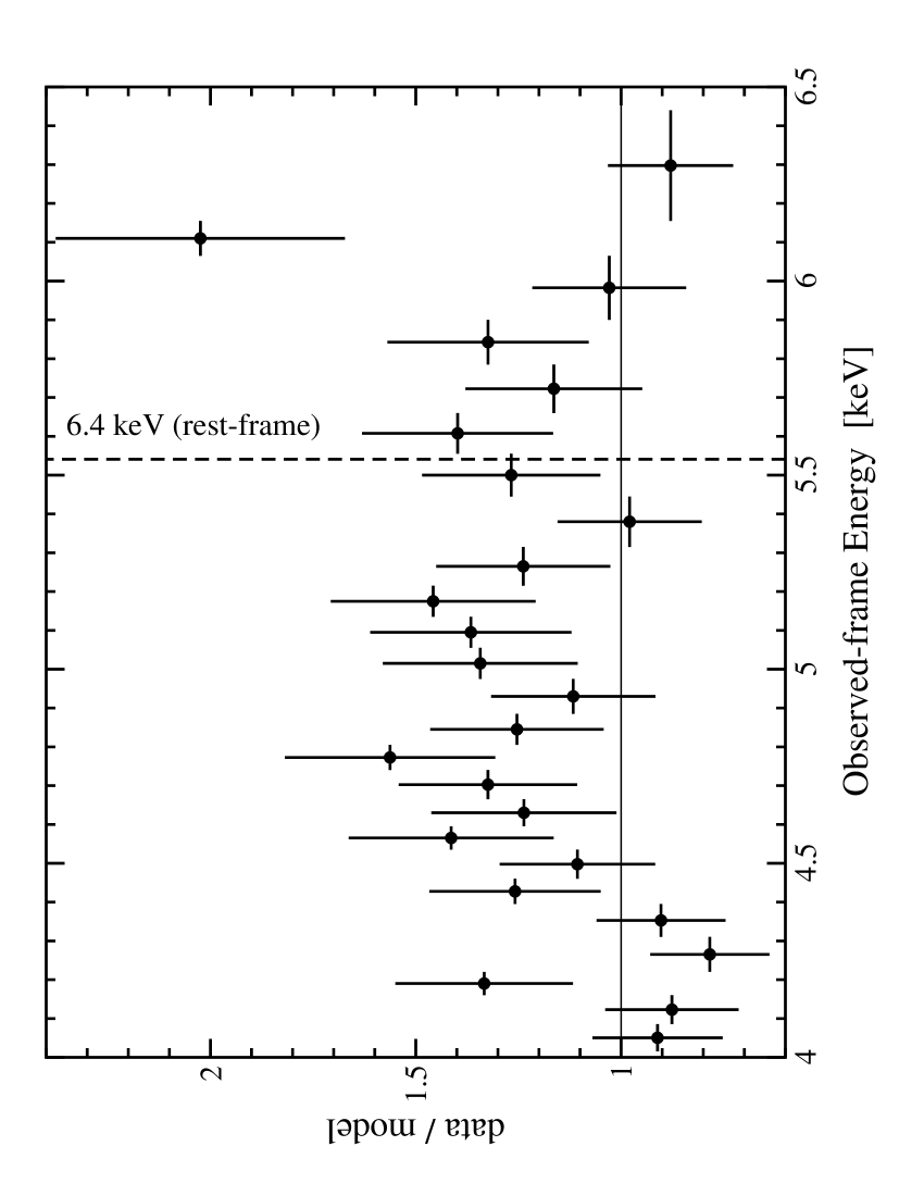
Figure 3: The pn residuals (data/model) in the intrinsic 4.6–7.5 keV range (a blow-up of the second top panel in Figure 2). The dashed vertical line is the 6.4 keV rest energy.

Since the excess is strongly concentrated to the red side of 6.4 keV (Figure 3), relativistic effects were considered. The possibility that the emission feature arises from a disc around a Schwarzschild black hole (Fabian et al. 1989) was examined. The fit using the disc line was comparable to the Gaussian profile ($\Delta\chi^{2}=20.3$ for 3 additional free parameters). The best-fit line energy was $E=5.69^{+0.15}_{-0.10}$ keV with an equivalent width of $EW=455\pm 5$ eV. The shift of the line to energies lower than $6.4$ keV suggests that gravitational redshift effects may be dominating the emission. Given that the best-fit line energy did not correspond to iron emission, we fixed the energy to 6.4 keV and refit the disc line model by allowing the inner and outer disc radii to be free parameters. This fit was also acceptable ($\chi^{2}=525.8$ for $519~{}dof$), and indicated that the disc line was emitted from a small annulus between about 18–24 $R_{g}$. An annular emission region could be realised if a specific region of the disc is being illuminated for some period of time (e.g. Iwasawa et al. 1999). Iron emission from an accretion disc around a Kerr black hole (Laor 1991) was also acceptable ($\Delta\chi^{2}=16.1$ for 3 additional free parameters). The line energy and inner radius were fixed at $E=6.4$ keV and $R_{in}=1.235~{}R_{g}$ (the innermost stable orbit around a Kerr black hole). In this case only a lower-limit for the outer radius was measured ($R_{out}>14~{}R_{g}$). The best-fit line parameters are given in Table 2.

Recent observations of some Seyferts have revealed narrow emission lines at peculiar energies redward of 6.4 keV (Turner et al. 2004; Yaqoob et al. 2003; Guainazzi 2003; Turner et al. 2002). Dovčiak et al. (2004) explain these features as iron lines produced in a small range of radii by localised flares. The feature in NAB 0205+024 could also be fitted with a series of three emission lines with energies of $E\approx 5.45,5.95,6.59$ keV and unconstrained widths ($\Delta\chi^{2}=28.6$ for 9 additional free parameters). The lines were much stronger ($EW\approx 97-240$ eV) than the narrow lines discussed by the above authors which have typical equivalent widths of a few tens of eV. In addition, splitting the broad feature into three components was not required on a statistical basis.

A broad Gaussian emission profile was not statistically required by the MOS2 data; however the MOS2 data were consistent with the pn model. The broad feature was not detected by $ASCA$. Simulations of the $ASCA$ observation using the pn model show that this was a signal-to-noise issue.

Table 2: The best-fit line model parameters to the broad-band pn spectrum. For each model the parameters given (as required) are: the power-law photon index ($\Gamma$); line energy ($E$); line width ($\sigma$); disc inclination ($i$); inner ($R_{in}$) and outer ($R_{out}$) disc radius in units of gravitational radii ($R_{g}=Gm/c^{2}$); power-law dependency on the disc emissivity ($q$); equivalent width ($EW$); flux ($F$) in units of $\times 10^{-14}\hbox{${\rm\thinspace erg}{\rm\thinspace cm}^{-2}{\rm\thinspace s}^{-1}\,$}$. Parameters marked with the superscript $f$ are fixed as leaving them free did not improve the fits.

Gaussian	$\chi^{2}_{\nu}=1.01(520)$
	$\Gamma=2.47\pm 0.02$
	$E=5.87^{+0.29}_{-0.27}$ keV
	$\sigma=623^{+300}_{-237}$ eV
	$EW=515\pm 6$ eV; $F=8.46$
Disc-line	$\chi^{2}_{\nu}=1.01(519)$
	$\Gamma=2.45\pm 0.03$
	$E^{f}=6.4$ keV
	$q^{f}=-2$; $R_{in}=18^{+7}_{-12}~{}R_{g}$; $R_{out}=24^{+17}_{-6}~{}R_{g}$
	$i=31^{+5}_{-11}~{}degr$
	$EW=490\pm 11$ eV; $F=6.10$
Laor line	$\chi^{2}_{\nu}=1.01(520)$
	$\Gamma=2.47\pm 0.02$
	$E^{f}=6.4$ keV
	$q^{f}=3$; $R^{f}_{in}=1.235~{}R_{g}$; $R_{out}>14~{}R_{g}$
	$i=37^{+9}_{-14}~{}degr$
	$EW=868\pm 10$ eV; $F=9.13$

4 Timing Analysis

4.1 X-ray and optical light curves

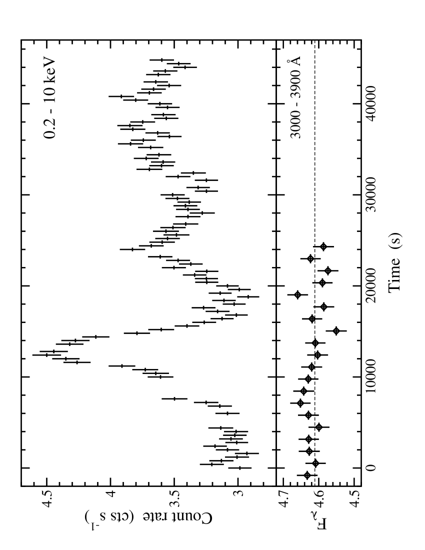
Figure 4: Top panel: The 0.2–10 keV light curve over the duration of the observation using 400 s bins. The time axis is defined from the start of the pn observation at 07:37:55 on 2002-07-23 UT. Bottom panel: The $U$-filter light curve obtained with the OM during the first $\sim 25$ ks of the observation. Flux-density units are $\times 10^{-15}\hbox{${\rm\thinspace erg}{\rm\thinspace s}^{-1}{\rm\thinspace cm}^{-2}{\rm\thinspace\AA}^{-1}\,$}$. A dashed line is drawn at the average flux density. The time axis is normalised to the pn start time.

The 0.2–10 keV light curve of NAB 0205+024 is displayed in the top panel of Figure 4 (with $1\sigma$ error bars). Since the broad-band light curve is less sensitive to calibration uncertainties the data between 0.2–0.3 keV have been included. In addition, the light curve from the entire observation is shown since the source is sufficiently brighter that the background (by about a factor of ten), even during the background flaring. The average count rate is $3.49\pm 0.10$ counts s^-1. The most striking feature is a flaring event about 10 ks into the observation in which the broad-band count rate increases by $\sim 50$% in a few thousand seconds. Averaging over three data points during flare maximum at $\sim 12.4$ ks and the three lowest data points when the flare achieves minimum intensity at $\sim 16.8$ ks results in a count-rate change of 1.33 counts s^-1 in 3800 s (rest-frame). Model (i) from Table LABEL:tab:cont is extrapolated down to 0.2 keV to estimate a 0.2–10 keV intrinsic luminosity of $7.74\times 10^{44}\hbox{${\rm\thinspace erg}{\rm\thinspace s}^{-1}\,$}$. Thus the calculated change in count rate corresponds to a luminosity change of $\Delta$L$=2.96\times 10^{44}\hbox{${\rm\thinspace erg}{\rm\thinspace s}^{-1}\,$}$ The luminosity rate of change is $\Delta$L/$\Delta$t $\approx$ 7.8 $\times$ 10⁴⁰ erg s^-2. Quantifying this rate of luminosity change in terms of a radiative efficiency, $\eta\mathrel{\hbox{\hbox to0.0pt{\hbox{\lower 4.0pt\hbox{$\sim$}}\hss}\hbox{$>$}}}4.8\times 10^{-43}$$\Delta$L/$\Delta$t (Fabian 1979), we calculate $\eta\mathrel{\hbox{\hbox to0.0pt{\hbox{\lower 4.0pt\hbox{$\sim$}}\hss}\hbox{$>$}}}0.037$. This is consistent with the efficiency of a Schwarzschild black hole.

A $U$-filter ($3000-3900{\rm\thinspace\AA}$) light curve was constructed from the OM data during the first $\sim 25$ ks of the observation (lower panel of Figure 4). In general, and in particular during the X-ray flare, the optical light curve shows no evidence of variability. A constant model fitted to the light curve was acceptable ($\chi^{2}_{\nu}=0.9$). In addition, two shorter light curves covering $\sim 5$ ks each were obtained with the $B$ ($3900-4900{\rm\thinspace\AA}$) and $UVW2$ ($1800-2250{\rm\thinspace\AA}$) filters. Neither of these curves showed any variability ($\chi^{2}_{\nu}<0.6$ for 4 $dof$ in each filter).

4.2 Spectral variablity

The fractional variability amplitude ($F_{var}$; Edelson et al. 2002) was calculated twice (Figure 5). Firstly, utilising data over the entire observation, and again while ignoring the data during the apparent flare ($\sim 10-15$ ks). As can be seen from Figure 5 the non-flare rms spectrum is consistent with a constant ($\chi^{2}_{\nu}=0.6$). On the other hand the flare data set shows clear spectral variability, with a gradual increase in the amplitude of the fluctuations with increasing energy. A constant fit is unacceptable ($\chi^{2}_{\nu}=6.8$).

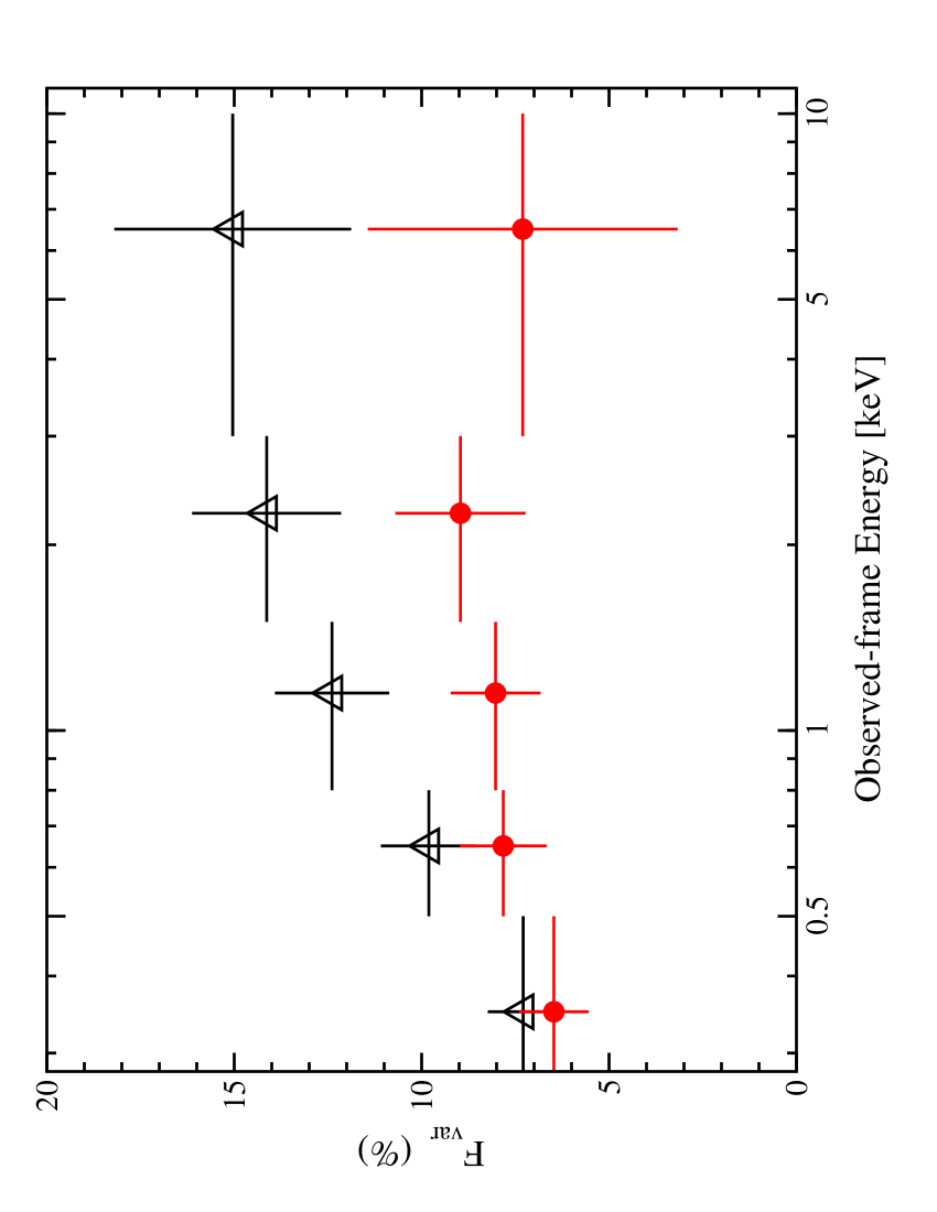
Figure 5: The RMS spectra of NAB 0205+024 over the entire observation (open, black triangles) and excluding the flaring event between $\sim 10-15$ ks (red dots). F_var is calculated using light curves in 1000 s bins.

Of interest is the notable similarity in the appearance and behaviour of the rms spectra with the rms spectra of another narrow-line quasar, I Zw 1 (Gallo et al. 2004). Gallo et al. also observed a flare in I Zw 1, of similar magnitude and duration to that seen in Figure 4. In addition, it was discovered that the flare in I Zw 1 was concentrated in the hard energy band (i.e. 2–10 keV), and that it induced spectral variability as suggested by Figure 5.

In Figure 6 we present normalised light curves in the 0.2–0.5 keV and 2–10 keV bands. The light curves were normalised to the average count rate during the non-flare periods (i.e. excluding the data between $\sim 10-15$ ks). As in I Zw 1, the flare appears to be concentrated in the harder energy band (though much less significant than for I Zw 1). The hardness ratio between the two light curves is also presented in Figure 6, and shows a difference in the hardness ratio before and after the flare.

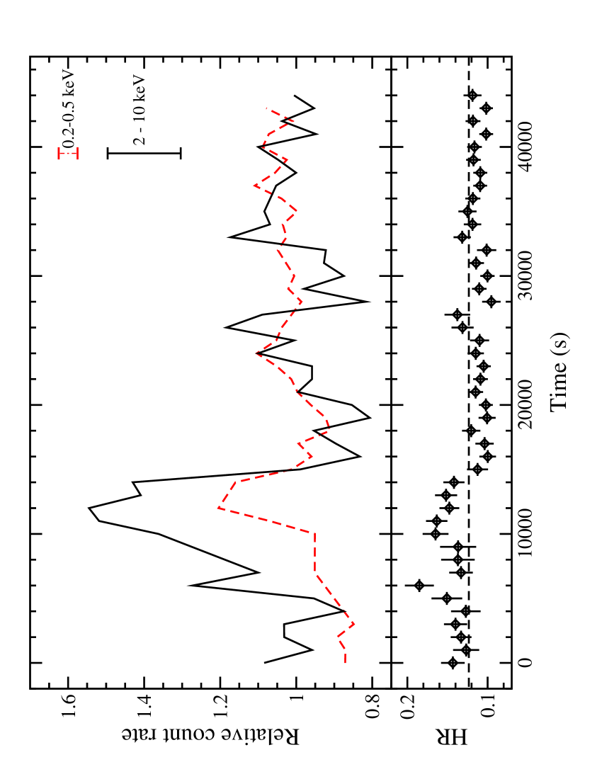
Figure 6: Top panel: Normalised light curves in the 0.2–0.5 keV (red, dashed curve) and 2–10 keV (black, solid curve) bands. The light curves were normalised to the average count rate during the non-flare periods (i.e. excluding the data between $\sim 10-15$ ks), to demonstrate the different flare amplitude in each band. The average size of the uncertainties for each curve are shown in the upper right of the panel. Bottom panel: The hardness ratio (HR = hard/soft) of the two light curves in the top panel as a function of time. Bin sizes are 1000s. A constant fit is drawn in as a dashed line.

Examining a “flaring” spectrum in detail is difficult due to the small number of good events in the first half of the observation. The mean spectrum is essentially dominated by the data in the post-flare regime (after $\sim 20$ ks).

5 Discussion and Conclusions

5.1 General Findings

The main results of this analysis are the following:

• The X-ray continuum of NAB 0205+024 was well fitted with a power-law plus blackbody with $\Gamma\approx 2.45$ and $kT\approx 120$ eV. Additional absorption above the Galactic column density was not required.
  

• A strong, broad feature was detected in the pn spectrum between 5–6 keV. A considerable amount of the emission, including the peak of the emission, is redward of 6.4 keV (rest-frame), and extends as far down as 5 keV in the rest-frame. The feature could be fitted as a neutral iron line emitted from a narrow annulus of a disc around a Schwarzschild black hole.
  

• A flare was detected in the light curve in which the broad-band count rate increased by about 50% in a few thousand seconds. The flare was determined to be concentrated at higher energies (2–10 keV) and appeared to induce spectral variability.
  

• No optical variability was detected from NAB 0205+024  even during the X-ray flare.

5.2 The nature of the high-energy emission line

Given the energy of the broad feature in NAB 0205+024  we considered the possibility that the broad line could be the composition of several narrower lines. Means to produce narrow emission lines in the 5–6 keV range have been suggested (e.g. Skibo 1997; Dovčiak et al. 2004); however the hypothetical narrow features in NAB 0205+024 do not satisfy these models physically (e.g. lines are too strong, or absence of accompanining features, or inconsistent relative abundances). Moreover, there was no statistical necessity to split the broad feature into multiple components.

The excess emission at $\sim 5$ keV can be fitted as neutral iron emitted from an accretion disc around a Schwarzschild or Kerr black hole. The fits cannot distiguish between the different line origins. In the case of a Schwarzschild black hole the line would originate from a thin annulus ($18-24~{}R_{g}$) close to the black hole. The feature could be fitted equally well with a simple Gaussian profile, but the best-fit energy and width do not correspond with the characteristics of any elements in the region.

5.3 A comparison to MCG–6-30-15 and I Zw 1

There are three significant differences in the XMM-Newton observation of NAB 0205+024 since it was last observed with $ASCA$ (Fiore et al. 1998; Leighly 1999a,b; Vaughan et al. 1999; Reeves & Turner 2000). Firstly, the power-law slope is notably softer in this observation ($\Gamma\approx 2.45$) compared to the $ASCA$ spectrum ($\Gamma\approx 2.09-2.22$). Secondly, there was no detection of a broad emission feature in the earlier observations, though at low significance there did appear to be spectral hardening with increasing energy (Fiore et al. 1998). Finally, a (hard) X-ray flare was detected with XMM-Newton.

There was also weak evidence for a temperature change in the blackbody component. The temperature measured by $ASCA$ was between 160–220 eV, whereas the temperature was much lower in the XMM-Newton data ($kT\approx 120$ eV). The reliability of the measured change is questionable given that $ASCA$ was not sensitive below $\sim 0.6$ keV, and due to the large range of temperatures measured in three different analyses of the same data. The average 0.6–10 keV XMM-Newton flux was about 15% lower compared to the $ASCA$ flux; however variations on this order are typical on hourly time scales.

The three new features are reminiscent of the second $ASCA$ observation of MCG–6-30-15 during which part of the time the broad line was found redshifted below 6 keV with no component detected at 6.4 keV, and the continuum appeared unusually soft (Iwasawa et al. 1999). Those authors interpreted the strange line emission as arising from an extraordinarily large gravitational redshift resulting from a flare occuring within $5~{}R_{g}$ of the black hole.

There is ample evidence for spectral softening in AGN during periods of increased 2–10 keV intensity (e.g. Done, Madejski & Zycki 2000; Vaughan & Edelson 2001). Merloni & Fabian (2001) have described this in terms of a ‘thundercloud’ model where a heating event in a compact region of the corona, likely due to magnetic reconnection (e.g. Galeev, Rosner & Vaiana 1979), results in an avalanche of smaller events. As the hard X-ray emission is reprocessed in the disc softer spectra are produced and the luminosity of the iron line is enhanced. The scenario appears applicable here, though it is difficult to examine in detail given the limited amount of data. The softer average spectrum (dominated by the post-flare data), the hard X-ray flare, and the iron line possibly emitted from an annular region are all consistent with the thundercloud model.

In this sense the flare observed in I Zw 1 (Gallo et al. 2004) is different in that no variability in the power-law slope, or enhancement of the iron line emission were detected. This can still be understood in terms of the thundercloud model if the I Zw 1 flare originated closer to the disc, but farther from the black hole. Thus, the flare illuminated a smaller portion of the disc, and spectral changes were smeared out in the mean spectrum. Support in favour of this scenario was the non-detection of a lag between energy bands in the I Zw 1 flare.

In this most recent and sensitive X-ray observation of NAB 0205+024, this narrow-line quasar has exhibited many differences since last observed with $ASCA$. The thundercloud model (Merloni & Fabian 2001) can be invoked to explain the hard X-ray flare, soft 2–10 keV power-law, and broad iron emission. Whether we examine narrow-line quasars or NLS1, it is becoming quite clear that these objects are important to understand the relativistic effects close to the black hole.

References

- [1] Arnaud K., 1996, in: Astronomical Data Analysis Software and Systems, Jacoby G., Barnes J., eds, ASP Conf. Series Vol. 101, p17
- [2] Bahcall, N. A., Bahcall J. N., Schmidt M., 1973, ApJ, 183, 777
- [3] Boller Th., Brandt W. N., Fink H., 1996, A&A, 305, 53
- [4] Boroson T. A., Green R. F., 1992, ApJS, 80, 109
- [5] Boroson T. A., 2002, ApJ, 565, 78
- [6] Brandt W. N., Mathur S., Elvis M., 1997, MNRAS, 285, 25
- [7] den Herder J. W., et al. 2001, A&A, 365, L7
- [8] Dickey J. M., Lockman F. J., 1990, ARA&A, 28, 215
- [9] Dovčiak M., Bianchi S., Guainazzi M., Karas V., Matt G., 2004, MNRAS, 350, 745
- [10] Done C., Madejski G. M., Zycki P. T., 2000, ApJ, 536, 213
- [11] Edelson R., Turner T.J., Pounds K., Vaughan S. Markowitz A., Marshall H., Dobbie, P., Warwick R., 2002, ApJ, 568, 610
- [12] Fabian A. C., 1979, Proc. R. Soc. London, Ser. A, 366, 449
- [13] Fabian A. C., Rees M. J., Stella L., White N. E., 1989, MNRAS, 238, 729
- [14] Fiore F., Elvis M., McDowell J. C., Siemiginowska A., Wilkes B. J., 1994, ApJ, 431, 515
- [15] Fiore F., et al. 1998, MNRAS, 298, 103
- [16] Galeev A. A., Rosner R., Vaiana G. S., 1979, ApJ, 229, 318
- [17] Gallo L. C., Boller Th., Brandt W. N., Fabian A. C., Vaughan S., 2004, A&A, 417, 29
- [18] Grupe D., 2004, AJ, 127, 1799
- [19] Guainazzi M., 2003, A&A, 401, 903
- [20] Iwasawa K., Fabian A. C., Young A. J., Inoue H., Matsumoto C., 1999, MNRAS, 306, L19
- [21] Jansen F. et al. 2001, A&A, 365, L1
- [22] Kirsch, M. 2003, XMM-Newton Calibration Presentations (CAL-TN-0018-2-1)
- [23] Klimek E. S., Gaskell C. M., Hedrick C. H., 2004, ApJ, 609, 69
- [24] Laor A., 1991, ApJ, 376, 90
- [25] Leighly K. 1999a, ApJS, 125, 317
- [26] Leighly K. 1999b, ApJS, 125, 297
- [27] Mason, K. O., Breeveld, A., Much, R., et al. 2001, A&A, 365, 36
- [28] Merloni A., Fabian A. C., 2001, MNRAS, 328, 958
- [29] Nicastro F., Fiore F., Matt G., 1999, ApJ, 517, 108
- [30] Osterbrock D. E., Pogge R. W., 1985, ApJ, 297, 166
- [31] Pollock 2003, XMM-Newton Calibration Presentations (CAL-TN-0030-2-1)
- [32] Reeves J. N., Turner M. J. L., 2000, MNRAS, 316, 234
- [33] Skibo J. G., 1997, ApJ, 478, 522
- [34] Strüder L. et al. 2001, A&A, 365, L18
- [35] Sulentic J. W., Zwitter T., Marziani P., Dultzin-Hacyan, D., 2000, ApJ, 536, 5
- [36] Turner M. J. L., Abbey A., Arnaud M., Balasini M. Barbera M., Belsole, E., Bennie P. J., Bernard J. P., Bignami G. F., Boer M. et al., 2001, A&A, 365, 27
- [37] Turner T. J. et al. 2002, ApJ, 574, L123
- [38] Turner T. J., Kraemer S. B., Reeves J. N., 2004, ApJ, 603, 62
- [39] Vaughan S., Reeves J., Warwick R., Edelson R., 1999, MNRAS, 309, 113
- [40] Vaughan S., Edelson R., 2001, ApJ, 548, 694
- [41] Yaqoob T., George I. M., Kallman T. R., Padmanabhan U., Weaver K. A., Turner T. J., 2003, ApJ, 596, 85