An Empirical Algorithm for Broad-band Photometric Redshifts of Quasars from the Sloan Digital Sky Survey

Abstract

We present an empirical algorithm for obtaining photometric redshifts of quasars using 5-band Sloan Digital Sky Survey (SDSS) photometry. Our algorithm generates an empirical model of the quasar color-redshift relation, compares the colors of a quasar candidate with this model, and calculates possible photometric redshifts. Using the 3814 quasars of the SDSS Early Data Release (EDR) Quasar Catalog to generate a median color-redshift relation as a function of redshift we find that, for this same sample, 83% of our predicted redshifts are correct to within $|\Delta z|<0.3$. The algorithm also determines the probability that the redshift is correct, allowing for even more robust photometric redshift determination for smaller, more restricted samples. We apply this technique to a set of 8740 quasar candidates selected by the final version of the SDSS quasar-selection algorithm. The photometric redshifts assigned to non-quasars are restricted to a few well-defined values. In addition, 90% of the objects with spectra that have photometric redshifts between 0.8 and 2.2 are quasars with accurate ($|\Delta z|<0.3$) photometric redshifts. Many of these quasars lie in a single region of color space; judicious application of color-cuts can effectively select quasars with accurate photometric redshifts from the SDSS database — without reference to the SDSS quasar selection algorithm. When the SDSS is complete, this technique will allow the determination of photometric redshifts for $\sim 10^{6}$ faint SDSS quasar candidates, enabling advances in our knowledge of the quasar luminosity function, gravitational lensing of quasars, and correlations among quasars and between galaxies.

1 Introduction

A photometric redshift (photo-$z$) is derived from the colors and morphology of an object, rather than from its spectrum. Since the bandwidth of an imaging filter is typically $\sim 1000$ Å while that of a spectroscopic exposure is more like $\sim$ 1–10 Å, it is much faster to obtain an image than to take a spectrum, and thus photometric redshift determination has the potential for determining reasonably accurate redshifts for large numbers of objects with a minimum of telescope time. In recent years, this technique has been applied to galaxies with great success (e.g., Brunner et al. 1997; Connolly et al. 1999; Mobasher et al. 2004; Benítez et al. 2004) as a result of the strong, discontinuous features found in the spectra of galaxies, such as the 4000 Å break, which cause galaxy colors to change substantially with redshift.

High-redshift quasars have a similar discontinuity as a result of hydrogen absorption blueward of Ly$\alpha$ emission (i.e., the Ly$\alpha$ forest; Lynds 1971) that allows for rough determination of their redshifts from broad-band photometry (e.g., Cristiani et al. 2004). Lower redshift quasars lack such a strong discontinuity in optical bands, but structure in the color-redshift relation caused by strong emission lines can be used to determine accurate photometric redshifts if the errors in the photometry are sufficiently small.

Early attempts at determining photometric redshifts for quasars are described by Hatziminaoglou, Mathez, & Pelló (2000) and Wolf et al. (2001) — demonstrating a success rate of roughly 50% (within $|\Delta z|<0.3$) for a few dozen quasars. The 17-filter COMBO-17 survey has had more success — identifying 192 $1.2\leq z\leq 4.8$ quasars with an expected photometric redshift accuracy of $\sigma_{z}=0.03$ (Wolf et al. 2003). Richards et al. (2001b) and Budavári et al. (2001) described two techniques for determining photometric redshift of quasars from the Sloan Digital Sky Survey (SDSS; York et al. 2000) imaging data. In this paper we expand and improve upon the empirical method that Richards et al. (2001b, hereafter RW01) applied to the SDSS photometry of 2625 quasars and Seyferts presented in Richards et al. (2001a).

In § 2 we review the details of the SDSS data and previous photo-$z$ attempts for quasars. Section 3 describes our current photometric redshift algorithm and how it differs from the original one presented in RW01. In §§ 4 and 5, we test our algorithm with two sets of SDSS data, each superior to that used in RW01. Section 5 also discusses practical applications of this approach. Section 6 summarizes our work.

2 Previous Attempts at Photometric Redshifts Using SDSS Imaging Data

This work, RW01, and Budavári et al. (2001) determine photometric redshifts for quasars by taking advantage of the quantity and quality of the imaging data from the SDSS. The SDSS obtains imaging data using a wide-field multi-CCD camera (Gunn et al. 1998) with five broad bands ($ugriz$; Fukugita et al. 1996). The photometric calibration of these data is described by Hogg et al. (2001), Smith et al. (2002), and Stoughton et al. (2002). Throughout this work we use point-spread-function “asinh” magnitudes (Lupton, Gunn, & Szalay 1999) that have been corrected for Galactic reddening (Schlegel, Finkbeiner, & Davis 1998). Richards et al. (2002) present the quasar selection algorithm, while Schneider et al. (2003) present the most recent catalog of bona-fide SDSS quasars. The SDSS’s tiling algorithm and astrometric accuracy are described by Blanton et al. (2003) and Pier et al. (2003), respectively. Further details related to Data Releases One (DR1) and Two (DR2) can be found in Abazajian et al. (2003) and Abazajian et al. (2004).

The 2625 quasars used in RW01 and Budavári et al. (2001) were not chosen with one uniform quasar-selection algorithm (the quasar selection procedure was under development at the time), but all of the objects had spectra as well as SDSS photometry. The empirical photometric redshift algorithm applied by RW01 minimized the $\chi^{2}$ between the observed and median colors of quasars as a function of redshift. It correctly predicted the redshifts of 55% of the objects to within 0.1, and 70% to within 0.2, a significant advance compared to previous work on this subject — both in sample size and accuracy.

RW01 pointed out some problem areas for future work on their algorithm. “Reddened quasars” (see Richards et al. 2003 and Hopkins et al. 2004) usually had incorrect photometric redshifts. Objects with an extended morphology also were more likely to yield incorrect redshift predictions. In addition, it was found that quasars at certain specific redshifts below 2.2 had nearly identical colors (“color-redshift degeneracies”), where the photometric redshift algorithm would sometimes select the incorrect value. RW01 discussed some improvements (e.g., weighting by redshift and assigning probabilities to the photometric redshifts) that could be made to the algorithm. This paper describes some of those improvements.

The photometric redshift tests in RW01 were performed with quasars whose redshifts were already spectroscopically known, but of course the ultimate goal is to apply the technique to quasar candidates that do not have spectra. Two solutions to the problem of accounting for non-quasars in the sample were suggested in RW01. First, it might be possible to differentiate between quasars and non-quasars using their photometric redshifts; perhaps most non-quasars would be assigned redshifts within a few narrow ranges that could be excluded a posteriori. Herein we test the accuracy of this suggestion. Second, it might be possible to select specific regions in color-space that have very high efficiency in quasar selection. We test this suggestion for a small sample of objects from the SDSS Early Data Release (EDR; Stoughton et al. 2002) database, while Richards et al. (2004) describes a more powerful selection algorithm (in terms of completeness and efficiency of quasar selection) using a much larger sample from the DR1 database.

3 The Algorithm

Suppose we have two sets of quasars, designated as $\mathcal{S}$ and $\mathcal{P}$. Those in set $\mathcal{S}$ have spectra, so we know each one’s redshift, $z_{\mathrm{spec}}$. We also have photometry for these quasars, as measured by the Sloan Digital Sky Survey: five magnitudes $(u,g,r,i,z)$, and their one-sigma uncertainties $(\sigma_{u},\sigma_{g},\sigma_{r},\sigma_{i},\sigma_{z})$. The quasars in the other set, $\mathcal{P}$, have no spectra, only photometry. Our goal is to obtain photometric redshifts $z_{\mathrm{phot}}$ for each of the quasars in $\mathcal{P}$.

There are two primary steps to our algorithm. First one must construct an empirical color-redshift relation (CZR) using set $\mathcal{S}$. Then one uses this CZR to assign photometric redshifts to each of the quasars in $\mathcal{P}$. We give the details of these steps below (using the quasars of the EDR catalog for set $\mathcal{S}$).

3.1 Construction of the CZR from the Quasars in $\mathcal{S}$

To begin, we sort the quasars of $\mathcal{S}$ into $N$ redshift bins. As in RW01, we chose bins with centers at intervals of 0.05 in redshift, and widths of 0.075 for $z_{\mathrm{spec}}<2.15$, 0.2 for $2.15\leq z_{\mathrm{spec}}<2.5$, and 0.5 for $z_{\mathrm{spec}}\geq 2.5$. The bins overlap, and become wider for higher redshift, in order to maintain enough quasars in each bin.

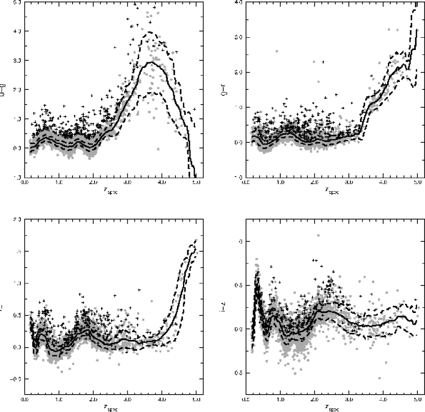
Figure 1: SDSS colors vs. spectroscopic redshift for EDR quasars, with CZR superimposed. Gray points: non-reddened quasars, black pluses: reddened quasars, solid line: mean color of CZR ($M_{i}^{j}$) for each redshift bin, dashed lines: 1-$\sigma$ range of uncertainty in CZR colors ($M_{i}^{j}\pm\sqrt{V_{i}^{jj}}$).

In Figure 1, we plot the SDSS colors of the EDR quasars as functions of spectroscopic redshift. Most quasars in a particular redshift bin have very similar colors, and it is this color-redshift relation that we wish to parameterize. However, there are a small fraction of quasars — plotted with black pluses — whose colors are significantly redder than they should be (compared to other quasars at the same redshift), especially in $u-g$ and $g-r$. We call these outliers to the CZR “reddened quasars” since they appear to be reddened by internal dust extinction (Richards et al. 2003). To prevent these quasars from skewing the CZR to the red, we exclude them from $\mathcal{S}$ before constructing the CZR.

3.1.1 Identification of the Reddened Quasars in $\mathcal{S}$

In this work, we defined reddened quasars using $u-g$ and $g-r$. Our reasoning was as follows: Figure 1 shows that $u-g$ colors can be significantly reddened. However, the uncertainties in $u-g$ are often quite large, due to the large uncertainties in SDSS $u$ magnitudes. Thus, we set a further constraint that reddened quasars should also be fairly red in $g-r$, the color that is second-most affected by the reddening. If a quasar’s $u-g$ color is redder than 97.5% of the other quasars in the same redshift bin, and its $g-r$ color is redder than the median $g-r$ color for its redshift bin, then we consider it to be a reddened quasar, and exclude it from set $\mathcal{S}$.

Recently, Richards et al. (2003) have shown that a more effective method for isolating reddened quasars is to make a cut on $\Delta(g-i)$: the $g-i$ color relative to the mean $g-i$ color at that redshift. In addition it may not be necessary to exclude reddened quasars at all if modal colors (Hopkins et al. 2004) are used to determine the CZR, since these colors should be unaffected by reddened outliers. We may alter our algorithm in the future to take these developments into account, but our definition of reddened quasars suffices for our purposes.

3.1.2 Parameterizing the CZR

Now that we have excluded the most heavily reddened quasars, we use the remaining quasars in set $\mathcal{S}$ to construct the CZR. In what follows, the index $i=1,\ldots,N$ will refer to the redshift bins. Let $Q_{i}$ be the number of non-reddened quasars in the $i^{\mathrm{th}}$ redshift bin; then the index $q=1,\ldots,Q_{i}$ ranges over the non-reddened quasars in that bin.

Using the colors of the quasars in the $i^{\mathrm{th}}$ bin, we calculate the mean color vector $\mathbf{M}_{i}$ and the color covariance matrix $\mathbf{V}_{i}$ for that bin. The four components of $\mathbf{M}_{i}$ are:

$$M_{i}^{j}=\frac{1}{Q_{i}}\sum_{q=1}^{Q_{i}}x_{j,q}\hskip 28.45274pt(j=1,2,3,4)$$

and the sixteen components of $\mathbf{V}_{i}$ are:

$$V_{i}^{jk}=\frac{1}{Q_{i}-1}\sum_{q=1}^{Q_{i}}(x_{j,q}-M_{i}^{j})(x_{k,q}-M_{i}^{k})\hskip 28.45274pt(j,k=1,2,3,4),$$

where $j$ and $k$ represent colors, and $x_{1,q}$, $x_{2,q}$, $x_{3,q}$, and $x_{4,q}$ are the $u-g$, $g-r$, $r-i$, and $i-z$ colors (respectively) of the $q^{\mathrm{th}}$ non-reddened quasar in the $i^{\mathrm{th}}$ redshift bin.

We then refine $\mathbf{M}_{i}$ and $\mathbf{V}_{i}$ by utilizing the following iterative procedure: (1) assume that the color distribution of the non-reddened quasars in the $i^{\mathrm{th}}$ bin is a four-dimensional multivariate normal distribution with mean $\mathbf{M}_{i}$ and covariance $\mathbf{V}_{i}$, (2) throw out any quasars in that bin with colors that lie in the outermost one percent of this hypothetical distribution, and (3) recalculate $\mathbf{M}_{i}$ and $\mathbf{V}_{i}$ for the remaining quasars in the bin. Repeat this procedure until $\mathbf{M}_{i}$ and $\mathbf{V}_{i}$ are unaltered; for the EDR data, we found that two iterations (removing roughly 7% of the non-reddened quasars) were sufficient.

The final $\mathbf{M}_{i}$ and $\mathbf{V}_{i}$, for all $i$, define the empirical color-redshift relation, or CZR. In Figure 1, we plot a representation of the CZR constructed from the non-reddened quasars in the EDR quasar catalog. In the four plots ($j=1,2,3,4$), $M_{i}^{j}$ (solid lines) and $M_{i}^{j}\pm\sqrt{V_{i}^{jj}}$ (dashed lines) are plotted versus redshift.

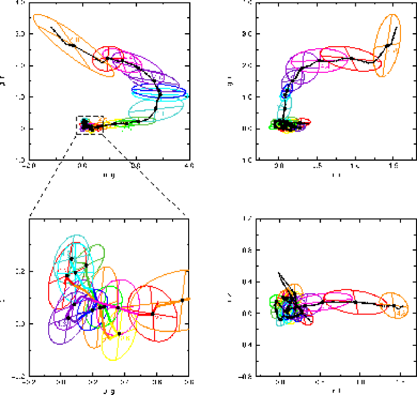
Figure 2: Color-space plot of CZR, as determined by the EDR quasars. Top-left, top-right, and bottom-right plots are two-dimensional projections of color-space — black dotted line: CZR track, colored ellipses: 1-$\sigma$ error ellipsoids of CZR for selected redshift bins, numbered points mark selected redshifts along the CZR. Bottom-left plot is an expansion of the indicated region in the top-left plot; the CZR track in this plot is colored to match the error ellipsoids. The dots are at intervals of 0.2 in redshift.

Another way to visualize the CZR is as a track in color-space, made of a series of four-dimensional multivariate Gaussian distributions (one for each redshift bin). Each Gaussian has an ellipsoidal cross-section. In Figure 2, we plot the EDR quasar CZR in two-dimensional projections of color-space. The CZR track for $z<2.2$ is completely contained in one small region of color-space $\sim 0.3$ magnitudes across. Quasars at these redshifts have similar colors, since the optical/UV continuum of a quasar spectrum is well-approximated by a power-law (which is invariant with redshift). This illustrates why it was so difficult to obtain photometric redshifts for these quasars using photographic plate photometry, with errors of $\sim 0.1$ magnitudes.

Now that we have constructed the CZR, we are ready to determine photometric redshifts.

3.2 Obtaining Photometric Redshifts for Quasars in $\mathcal{P}$

For a particular quasar in $\mathcal{P}$ for which we want to obtain a photometric redshift $z_{\mathrm{phot}}$, let the vector $\mathbf{X_{0}}$ be its observed colors $(u-g,g-r,r-i,i-z)$, and let the matrix $\mathbf{V_{0}}$ be the covariance matrix of its colors. The latter can be derived from the one-sigma uncertainties in its observed magnitudes $(\sigma_{u},\sigma_{g},\sigma_{r},\sigma_{i},\sigma_{z})$, assuming that the errors are uncorrelated with each other:

$$\begin{array}[]{ccc}\mathbf{V_{0}}&=&\left(\begin{array}[]{cccc}\sigma_{u}^{2}+\sigma_{g}^{2}&-\sigma_{g}^{2}&0&0\\ -\sigma_{g}^{2}&\sigma_{g}^{2}+\sigma_{r}^{2}&-\sigma_{r}^{2}&0\\ 0&-\sigma_{r}^{2}&\sigma_{r}^{2}+\sigma_{i}^{2}&-\sigma_{i}^{2}\\ 0&0&-\sigma_{i}^{2}&\sigma_{i}^{2}+\sigma_{z}^{2}\end{array}\right)\end{array}$$

We now compute the chi-square value, $\chi^{2}_{i}$, between the observed colors of the quasar, and the CZR’s $i^{\mathrm{th}}$ redshift bin:

$$\chi^{2}_{i}=(\mathbf{X_{0}}-\mathbf{M}_{i})^{T}(\mathbf{V_{0}}+\mathbf{V}_{i})^{-1}(\mathbf{X_{0}}-\mathbf{M}_{i})\hskip 28.45274pt(i=1,\ldots,N)$$

and from this $\chi^{2}$ value, derive the probability $P_{i}$ that the quasar’s redshift lies in the $i^{\mathrm{th}}$ redshift bin:

$$P^{\prime}_{i} = \frac{W_{i}\exp(-\chi^{2}_{i}/2)}{4\pi^{2}|\mathbf{V_{0}}+\mathbf{V}_{i}|^{1/2}}$$

$$P_{i} = \frac{P^{\prime}_{i}}{\sum_{i=1}^{N}P^{\prime}_{i}}\hskip 56.9055pt(i=1,\ldots,N),$$

where $P_{i}$ is normalized so that its sum over all $i$ is unity.

$W_{i}$ is the a priori probability that a quasar has a redshift in the $i^{\mathrm{th}}$ redshift bin. If the redshift distributions of $\mathcal{S}$ and $\mathcal{P}$ are expected to be similar, then $W_{i}$ is the fraction of quasars in $\mathcal{S}$ (both reddened and non-reddened) that lie in the $i^{\mathrm{th}}$ redshift bin; otherwise $W_{i}$ should be equal to $1/N$ for all $i$.

If the object is identified as an extended source by the SDSS photometric pipeline, it is probably at a redshift of less than one. In that case, we only calculate probabilities $P_{i}$ for the $N^{\prime}$ redshift bins that lie between $z=0$ and $z=1$ (where this upper limit is an argument to the algorithm), and $N$ is replaced with $N^{\prime}$ in the formulae for $P^{\prime}_{i}$ and $P_{i}$ above. (For an extended object, $W_{i}$ is handled in exactly the same way as it is for a point-source.) Of course there are dangers in taking this approach. For example, at fainter magnitudes the SDSS’s star-galaxy separation can break down, and superposition of sources can mimic extended objects.

Finally, to obtain a photometric redshift for the quasar, we search for groups of consecutive redshift bins for which each $P_{i}$ exceeds some threshold value (our choice was $1/N$). Each such group defines:

• a photometric redshift (the redshift bin in the group with the largest $P_{i}$),

• an approximate range to the photometric redshift (obtained from the lowest and highest redshifts in the group), and

• a probability (or “confidence-level”) that the actual redshift is within this range (the sum of $P_{i}$ for all redshift bins in the group).

One can either restrict one’s attention to the photometric redshift with the highest probability, or list multiple choices for the photometric redshift with their associated probabilities.

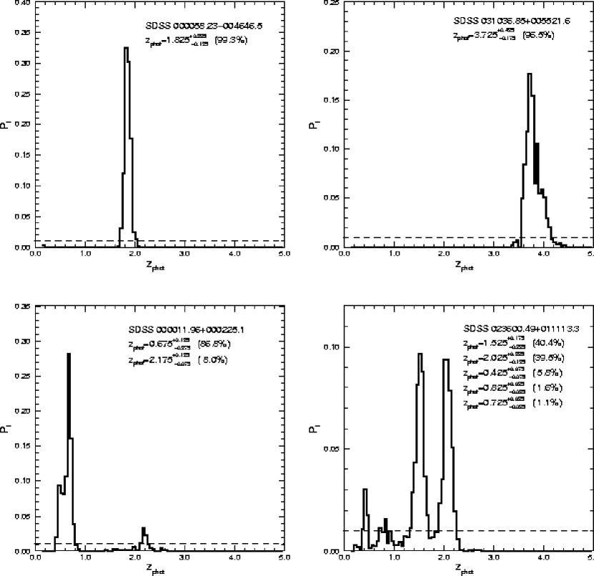
Figure 3: The probability distribution ($P_{i}$) for the photometric redshifts for four EDR quasars. The top two panels show objects with only one likely photo-$z$; the bottom two panels show examples of objects with more than one likely photo-$z$. For each quasar, the most likely photometric redshift(s) are given along with the range and confidence-levels. Their true redshifts are (clockwise from top-left): 1.896, 3.780, 1.81, and 0.479.

Figure 3 is an illustration of how to derive photometric redshifts from $P_{i}$. We display $P_{i}$ as a function of redshift for four EDR quasars. The dashed line is the threshold probability level of $1/N$. Each spike in $P_{i}$ which reaches above this threshold represents one possibility for $z_{\mathrm{phot}}$. For each quasar, the most likely photometric redshifts are listed, along with their ranges and confidence-levels. The top two quasars in the figure have only one likely photometric redshift each, while for the bottom two, there are several possible $z_{\mathrm{phot}}$.

3.3 Summary of Changes Made to the RW01 Algorithm

Between the publication of RW01 and now, we have made the following refinements to our original photo-$z$ algorithm:

• The empirical CZR is parameterized in a more refined way. It is now parameterized as a series of four-dimensional multivariate Gaussians with ellipsoidal cross-sections, one for each redshift bin. (Modulo a $\sim 10$% tail of red quasars, Richards et al. (2003) found that the color distribution of SDSS quasars is relatively Gaussian.) The variances of the Gaussians (which define the “width” of the CZR) are allowed to change as a function of redshift. Also, the covariances of the Gaussians are taken into account, i.e.: the principal axes of the Gaussians’ ellipsoidal cross-sections are not required to be aligned with the four axes of color-space.

• The uncertainties in the observed colors of an individual quasar are handled more rigorously. The uncertainty in the $u-g$ color of a quasar is correlated with the uncertainty in its $g-r$ color (since both involve the quasar’s $g$-magnitude); in other words, the covariance between the quasar’s $u-g$ and $g-r$ colors is not zero. When finding the photometric redshift of a particular quasar, we therefore consider the full covariance matrix (covariances as well as variances) for its observed colors. As a corollary to these first two refinements, the expression for the $\chi^{2}$ statistic is more complicated, as shown in Section 3.2.

• The photometric redshift of a quasar is now determined by maximizing its probability $P_{i}$, rather than minimizing its $\chi^{2}$ as a function of redshift. Now that we allow the width of the CZR to vary with redshift, it is no longer true that $P_{i}$ is solely related to $\chi^{2}_{i}$; it also depends on the covariance matrix of the CZR. For this reason, we can no longer let $\chi^{2}$ minimization stand in for probability maximization, but rather we must let the latter determine the photometric redshift.

• We can optionally take into account the fact that certain quasar redshifts are more likely than others, if that knowledge is available a priori. For instance, suppose we have a large set of quasars for which we wish to find photometric redshifts, and for some small subset of these quasars we have spectra and therefore know their spectroscopic redshifts. As long as this subset was chosen in an unbiased way, it is reasonable to assume that the redshift distribution of all the quasars is identical to the redshift distribution of the subset. Thus, we can weight the photometric redshift probabilities $P_{i}$ by the redshift distribution of the subset, so that certain redshifts will be favored more than others.

• If a quasar candidate is detected as an extended source by the SDSS photometric pipeline (Lupton et al. 2001), its redshift is probably $\lesssim 1$. In the current photometric redshift technique, we only consider redshifts less than 1 for the $z_{\mathrm{phot}}$ of an extended object.

4 Tests of the Algorithm Using Confirmed Quasars

4.1 Efficiency of the Algorithm on Known Quasars

To compare the efficiency of the new photometric redshift algorithm with that of the one from RW01, the algorithm was tested on the Early Data Release Quasar Catalog (Schneider et al. 2002). This catalog consists of 3814 quasars with both SDSS photometry and spectra. Unlike the set of 2625 quasars and Seyferts that we used to test the earlier version of the algorithm in RW01, all of the EDR quasars have at least one emission line with FWHM $>1000$ km s^-1, a luminosity of $M_{i}<-23$, and very reliable redshifts. (It should be noted, however, that neither data set is statistically homogeneous, since the quasar-selection algorithm was still undergoing changes and improvements while these data-sets were being made; see Stoughton et al. 2002.) Although there exist newer data than the EDR data, the number of objects with redshifts and the quality of their photometry are more than sufficient for our tests. Furthermore, similar results are obtained for a much larger sample of DR1 objects analyzed by Richards et al. (2004).

4.1.1 Tests where $\mathcal{S}$ and $\mathcal{P}$ are identical

After constructing a CZR from the 3814 EDR quasars, the photo-$z$ algorithm was run on the same set of quasars; these photometric redshifts were compared to the true, spectroscopic redshifts. Since, for these tests, $\mathcal{S}$ and $\mathcal{P}$ are identical, we used $W_{i}$ to weight $P_{i}$ by the redshift distribution of the EDR quasars.

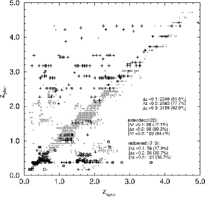
Figure 4: Photometric redshift vs. spectroscopic redshift for the 3814 EDR quasars. Gray circles: non-reddened quasars, black pluses: reddened quasars, black squares: extended quasars.

Figures 4 and 5 show the results of this exercise. In Figure 4, we plot the most probable photometric redshift $z_{\mathrm{phot}}$ of each quasar against its spectroscopic redshift $z_{\mathrm{spec}}$. Most of the photometric redshifts agree well with the spectroscopic redshifts, with incorrect photometric redshifts generally coming in the form of degeneracies between very different redshifts (e.g., between $z=0.6$ and $z=1.6$) or from “smearing” of nearby redshifts (e.g., $z_{\mathrm{phot}}\sim 1.4$). Of the 3814 quasars, the number (percent) with photometric redshifts that were correct to within 0.1, 0.2, and 0.3 were: 2348 (61.6%), 2963 (77.7%), and 3159 (82.8%), respectively. This result should be compared to the corresponding result in RW01 (using the old version of the algorithm), where only 70.0% of the quasars’ photometric redshifts were correct to within 0.2. In Figure 5, we plot a histogram of $\Delta z=z_{\mathrm{spec}}-z_{\mathrm{phot}}$ for these same quasars.

As discussed in Section 3.2, our photometric redshift algorithm supplies not only a value for each quasar’s $z_{\mathrm{phot}}$, but a range around that $z_{\mathrm{phot}}$, and an associated confidence-level (the probability that the spectroscopic redshift is within the range). For example, the photometric redshift of a quasar might be given as $2.35^{+0.10}_{-0.15}$, to 85% confidence. Of the 3814 EDR quasars, the spectroscopic redshift lies within the range for 3176 of them (83.3%). Figure 6 shows the distribution of range sizes. The median range size is 0.42, and 90% of the ranges are smaller than 0.64. Thus most of our $z_{\mathrm{phot}}$ error bars are $\pm 0.3$ or smaller.

We test the confidence level supplied with the photometric redshifts in the following manner. Consider all of the quasars whose photometric redshift ranges have associated confidence levels of (say) 50-55%. One would expect that roughly 50-55% of these quasars would have their spectroscopic redshifts within the given range, if the confidence level was reliable. Figure 7 shows that the confidence levels pass this test very well, especially when there are many quasars with the same confidence level: roughly $x$% of the objects with $x$% confidence level have a spectroscopic redshift within the range.

4.1.2 Tests where $\mathcal{S}$ and $\mathcal{P}$ are different

In any practical application of the photometric redshift algorithm, $\mathcal{S}$ and $\mathcal{P}$ will not be identical sets. We therefore performed two more tests using the EDR quasars, to measure the efficiency of the method in this more realistic case.

In the first test, we randomly chose 954 (25%) of the EDR quasars from which to construct the CZR. This CZR was used to predict photometric redshifts for the remaining 2860 EDR objects. Since in this case $\mathcal{S}$ and $\mathcal{P}$ are both drawn from the EDR quasars, the redshift distributions of the two sets will be the same. So for this test, we weighted the photometric redshifts of the quasars in $\mathcal{P}$ by the redshift distribution of the quasars in $\mathcal{S}$. Of the 2860 quasars, the number (percent) of them with photometric redshifts correct to within 0.1, 0.2, and 0.3 are: 1598 (55.9%), 2136 (74.7%), and 2312 (80.8%), respectively. The efficiency of the method is nearly as high as when the quasars in the CZR and the quasars being tested were identical.

In the second test, we made the CZR from the 2829 EDR quasars with $i<19$, and used it and our $z_{\mathrm{phot}}$ technique to obtain photometric redshifts for the 985 $i>19$ objects. For this test, the redshift distributions of $\mathcal{S}$ and $\mathcal{P}$ are not necessarily the same. Therefore, we did not weight the photometric redshifts by the redshift distribution of the CZR. Of the 985 EDR quasars with $i>19$, the number (percent) of them with photometric redshifts correct to within 0.1, 0.2, and 0.3 are: 499 (50.7%), 681 (69.1%), and 733 (74.4%), respectively. These efficiencies are somewhat lower than those of the previous tests, because all of the objects in $\mathcal{P}$ are faint, and thus have larger photometric uncertainties. Nevertheless, the results are still quite good compared with previous work in this field.

4.1.3 Tests Using Multiple CZRs

Another test worth mentioning is one where instead of comparing the colors of input objects to a single CZR, we compared colors to multiple CZRs defined as a function of their broad spectral slope. Specifically, we created multiple CZRs for quasars as a function of their $\Delta(g-i)$ colors. We can then determine photometric redshifts with respect to each of these CZRs. This approach is motivated by the finding of Richards et al. (2003) that quasars with different optical colors have somewhat different emission line properties. Unfortunately, we found that using multiple CZRs did not help and we will hereafter only consider photometric redshifts derived from comparisons to the single median CZR.

4.2 Problematic Quasars

4.2.1 Extended Quasars

In Figure 4, the 122 black squares are quasars that were classified as “extended” (i.e., not a point source) by the SDSS photometric pipeline (Lupton et al. 2001) based on a comparison of PSF and model magnitudes. Most of these objects have $z_{\mathrm{spec}}<1$ as expected, justifying our weighting of extended sources to low redshift. Extended objects with spectroscopic redshifts larger than 1 are most likely either lensed quasars, star-quasar superpositions, or galaxy-quasar superpositions. Any of these, if unresolved, could be mistaken for a single extended source.

Our use of PSF magnitudes will partially mitigate the effects of the host galaxy, but the PSF quasar photometry is still influenced by host galaxy light for extended sources. Host galaxy light will alter the observed colors of the quasars, which would cause a problem with obtaining accurate photometric redshifts. Indeed, when the earlier version of our $z_{\mathrm{phot}}$ algorithm (presented in RW01) was applied to the EDR quasars, 46 out of the 122 extended quasars (37.7%) had $|\Delta z|>0.3$; most of these were assigned photometric redshifts greater than one.

By restricting the redshift range of extended sources, there are now only 19 extended quasars with incorrect photometric redshifts. Since 16 have $z_{\mathrm{spec}}>1$, we are really missing only three quasars. (Of course, the 27 extended quasars recovered in this way are negligible compared to the 3814 quasars in the entire sample, so our overall efficiency only increased by a fraction of a percent.) Thus, it appears that we do not have to worry about getting incorrect photometric redshifts for extended quasars.

4.2.2 Reddened Quasars

Of the 3814 quasars in the EDR, 313 are reddened according to our definition; these are plotted with black pluses in Figure 4. Since these quasars have unusual colors for their redshifts, it is clear that their photometric redshifts will probably be incorrect. An examination of Figure 4 shows that this is indeed the situation; of the 313 reddened quasars, 192 of them (61.3%) have photometric redshifts with $|\Delta z|>0.3$.

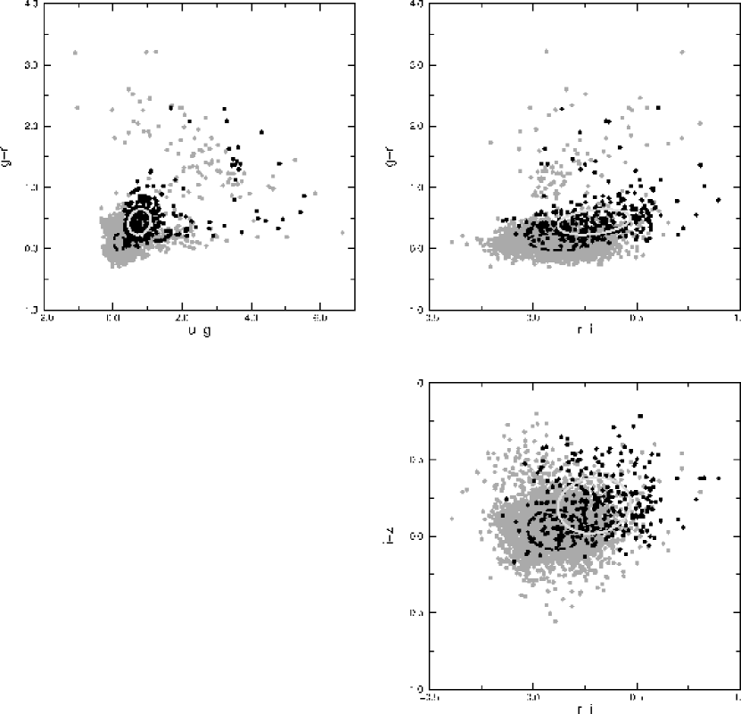
Figure 8: Distributions in color-space of non-reddened EDR quasars (gray points) and reddened EDR quasars (black points). Dashed black ellipses: projections of 1-$\sigma$ ellipsoid for non-reddened quasar distribution; solid gray ellipses: projections of 1-$\sigma$ ellipsoid for reddened quasar distribution.

Since the majority of reddened quasars will have incorrect $z_{\mathrm{phot}}$, we could increase the efficiency of our photometric redshift algorithm if they could be identified from photometric information alone, and excluded from the sample. Figure 8 shows the positions in color-space of the reddened quasars (black points) and the non-reddened quasars (gray points). For the most part, the non-reddened quasars are found in a four-dimensional ellipsoidal Gaussian, and the reddened quasars are in a second ellipsoidal Gaussian, substantially offset from the non-reddened one. (The quasars not found in the Gaussians are $z\gtrsim 2.5$ quasars, which have the Lyman $\alpha$ forest redshifted into the SDSS filters.)

Here we have a similar problem to that of finding photometric redshifts. In both cases, quasars of different kinds are found in roughly ellipsoidal Gaussians, separated from each other in color-space. If we quantify the positions, sizes, and shapes of the different Gaussians, we can calculate the probability that any particular object (a point in color-space) was drawn from one of the Gaussian distributions. Hence, we can use the photometric redshift technique itself (slightly modified) to obtain an approximate probability that a given quasar is reddened.

We used the CZR branch of the $z_{\mathrm{phot}}$ algorithm (see Section 3.1.2) to measure the ellipsoidal Gaussians for the reddened and non-reddened quasars. To remove the $z\gtrsim 2.5$ quasars, we ran ten iterations of the outlier-removing procedure (see § 3.1.2), instead of two. Projections of the derived Gaussians are plotted in Figure 8 with a dashed line (for the non-reddened quasars) and a solid line (for the reddened quasars).

We then used the last part of the $z_{\mathrm{phot}}$ algorithm (see Section 3.2) to calculate the probability, $P_{nr}$, that an EDR quasar belongs to the non-reddened distribution, and the probability, $P_{r}$, that it belongs to the reddened distribution (where $P_{nr}+P_{r}=1$). This was done for all 3814 EDR quasars. Since there are 11.2 times more non-reddened quasars than there are reddened quasars, we weighted $P_{nr}$ and $P_{r}$ accordingly.

We then can use $P_{r}$ to select out mostly non-reddened quasars. If we consider only the EDR quasars with $P_{r}<0.99$, we will have 3384 quasars, and only 106 of them (or 3.1%) will be reddened (a reduction in total sample size of 13% but a drop in the “contaminated fraction” from 8.2% to 3.1%). Subsets with a higher fraction of non-reddened quasars can be made by lowering the upper bound on $P_{r}$, although at the cost of making the subsets somewhat smaller; for example, there are only 2617 quasars with $P_{r}<0.01$, but only one of them is reddened.

Although we have not made such $P_{r}$ cuts in this paper, we see that $P_{r}$ can be used to largely eliminate reddened quasars using only photometric information. In future work, we will use $P_{r}$ to improve the efficiency of our photometric technique still further.

4.2.3 Color-redshift Degeneracies

Of the 655 EDR quasars with $|\Delta z|\geq 0.3$, 192 are reddened, and 19 are extended. That still leaves 444 “ordinary” quasars with incorrect $z_{\mathrm{phot}}$ — and many of these are really incorrect, with $|\Delta z|=1.0$ or even $2.0$!

An examination of Figure 4 shows that these quasars are placed roughly symmetrically about the $z_{\mathrm{phot}}=z_{\mathrm{spec}}$ diagonal. For instance, some quasars with $z_{\mathrm{spec}}=0.8$ are assigned a $z_{\mathrm{phot}}$ of 2.1, whereas some quasars with $z_{\mathrm{spec}}=2.1$ are given a $z_{\mathrm{phot}}$ of 0.8. This situation arises because there is considerable degeneracy in the color-redshift relation for $z\lesssim 2.5$ — i.e.: quasars at fairly different redshifts (like 0.8 and 2.1) can still have very similar colors. Color-redshift degeneracies occur when the CZR intersects itself (or does so very nearly) in color-space — see the inset of Figure 2 for an illustration of this.

When a quasar’s colors are consistent with two (or more) redshifts, the function $P_{i}$ (the probability that its redshift is in redshift bin $i$) has two or more peaks of roughly equal size, at each of the possible redshifts. An example is the bottom-right plot in Figure 3, which shows a degeneracy between $z=1.5$ and $z=2.0$ (easily seen in Figure 4). If the algorithm is looking for the most probable $z_{\mathrm{phot}}$, it may or may not pick the correct one. Fortunately, our algorithm can be directed to search out the $n$ most likely photometric redshifts, where $n$ is any desired integer. Thus, if we find that two or more choices for $z_{\mathrm{phot}}$ have similar confidence-levels, we at least know that one of them is probably correct (although we do not know which one!).

If $P_{i}$ is being weighted by the redshift distribution of the CZR, that may help the algorithm select the correct $z_{\mathrm{phot}}$. For instance, in the EDR, there are twice as many quasars with $z_{\mathrm{spec}}=1.5$ as there are with $z_{\mathrm{spec}}=2.0$. So even though quasars at either redshift have very similar colors, a quasar with these colors is twice as likely to have a redshift of 1.5, and the weighting of $P_{i}$ will reflect this. Of course, this will only work if the redshift distribution of $\mathcal{P}$ is similar to that of $\mathcal{S}$. It should also be noted that this weighting technique will be of most use if one is searching for the $n$ most likely photometric redshifts, and listing them by probability (as is done in Fig. 3). If one is only searching for the most likely photometric redshift, then the weighting will cause the algorithm to always select the more common redshift when faced with a true degeneracy (e.g., $z=1.5$ over $z=2.0$).

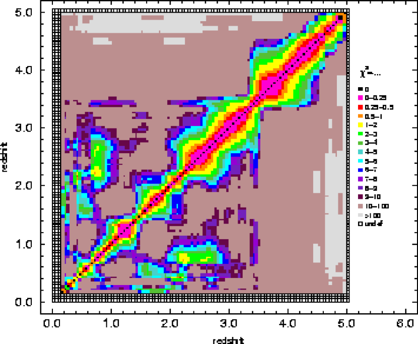
Figure 9: Degeneracy map for EDR CZR. Color of pixel at position $(x,y)$ represents $\chi^{2}$ “distance” in color-space between redshifts $x$ and $y$.

Since degenerate redshifts are found where the CZR intersects itself in color-space, we can create a map of the degenerate redshifts by measuring the “distance” in color-space between any two points on the CZR — the closer they are, the more degenerate the corresponding redshifts. Figure 9 is such a map.

In Figure 9, the color of the pixel at position $(x,y)$ represents the $\chi^{2}$ “distance” between redshift $x$ and redshift $y$ in the CZR. The smaller the value of $\chi^{2}$, the more similar the colors of quasars at these redshifts. Notice that the structure of Figures 4 and 9 are similar (modulo the fact that Figure 9 is symmetric by definition, whereas Figure 4 need not be). Thus, consulting this map is a way to determine whether or not a quasar with a certain $z_{\mathrm{phot}}$ has degenerate colors.

5 Tests of the Algorithm Using Quasar Candidates

In this section, we present a second round of tests, in which we apply our $z_{\mathrm{phot}}$ algorithm to quasar candidates selected by the final version of the SDSS quasar-selection algorithm. We call this data-set the Final Early Data Release (FEDR), since its objects are found in the same region of sky as the EDR. Many of these objects have no spectra, and a significant fraction of those that do are not quasars. We also introduce the concepts of the “Window” (a $z_{\mathrm{phot}}$ cut) and the “Box” (a series of color cuts) through which — by solely photometric means — we can select quasar candidates that are mostly quasars, the majority of which have accurate photometric redshifts.

Although the EDR quasar tests presented in § 4 are encouraging, and show that the photometric redshift algorithm is working well, they are not realistic exercises in that we already know that all 3814 objects are quasars. In a real application, the objects chosen to be quasar candidates (based on their photometry only) will include many non-quasars. The tests described in this section are designed to see what happens when our $z_{\mathrm{phot}}$ algorithm operates on more realistic data. For these tests, our CZR was, as before, constructed from the EDR Quasar Catalog. However, we then used this CZR to find photometric redshifts for the FEDR, a set of 8740 objects which we describe below. (Since in this case $\mathcal{S}$ and $\mathcal{P}$ probably do not have the same redshift distributions, we did not weight the photometric redshifts.)

5.1 FEDR, and How it Differs from the EDR Quasars

The FEDR is a set of quasar candidates from the same region of sky as the EDR quasars. The quasar-selection algorithm used to select these objects was the final, current version (discussed in Richards et al. 2002); as such these objects are statistically homogeneous, in contrast to the EDR quasars from Schneider et al. (2002). Since the FEDR objects were selected solely by photometric means, not all have spectra.

Of the 8740 objects, 3985 are of unknown type. (Most of these have no spectra; 22 have unidentifiable spectra.) The other 4755 were identified by the SDSS selection algorithm as: 52 “late-type” stars (type M, L, or T), 527 “regular” stars, 828 normal galaxies, and 3348 quasars and AGNs.

In presenting the results of the FEDR tests, we first consider how well the photometric redshift algorithm performed for 1) the 3348 FEDR objects known to be quasars, 2) the 1407 FEDR objects known to be non-quasars, and 3) the 3985 FEDR objects of unknown type.

5.2 Objects Confirmed to be Quasars

Of the 3348 objects spectroscopically confirmed to be quasars, the number (percent) with photometric redshifts that were correct to within 0.1, 0.2, and 0.3 were: 2156 (64.4%), 2692 (80.4%), and 2860 (85.4%), respectively. There were 2783 quasars (83.1%) whose spectroscopic redshifts lay within the photometric redshift ranges. The distribution of range sizes has a median of 0.39, and 90% of the ranges are smaller than 0.64. The confidence levels quoted for the photometric redshifts’ error bars appear to be reasonable. These results are quite similar to those found for the EDR quasars, not surprisingly given the degree of overlap in the two sets.

5.3 Objects that are Confirmed Non-Quasars

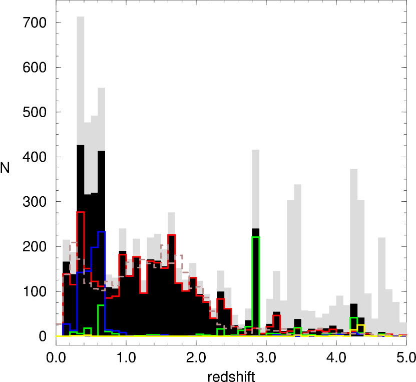
Figure 10: Distribution of photometric redshifts for the following types of objects in FEDR — all objects (gray), objects with spectra (black), quasars (red), stars (green), late-type stars (yellow), galaxies (blue). Brown, dashed histogram is distribution of spectroscopic redshifts for FEDR quasars.

Figure 10 is a histogram of the photometric redshifts for all 8740 objects. Grey bars show the $z_{\mathrm{phot}}$ distribution for all of the objects, including those that have no spectra, while black bars show the $z_{\mathrm{phot}}$ distribution for only the 4755 objects with spectra. The red, green, yellow, and blue histograms show the $z_{\mathrm{phot}}$ distributions for confirmed quasars, stars, late-type stars, and galaxies, respectively. The brown, dashed histogram shows the $z_{\mathrm{spec}}$ distribution of the 3348 confirmed quasars, for comparison.

Most of the photometric redshifts assigned to confirmed non-quasars take on a few specific values. Nearly all galaxies are assigned photometric redshifts between 0.3 and 0.7. Many stars receive a photometric redshift between 2.8 and 2.9; most others are found between 0.6 and 0.7, or between 4.2 and 4.3. Almost all late-type stars have a photometric redshift between 4.2 and 4.4. The color-space distributions of stars and galaxies intersect (or at least approach) the quasar CZR at these specific redshift values. Also, there are almost no non-quasars assigned photometric redshifts between 0.8 and 2.2.

These results are very encouraging. Suppose one uses the SDSS quasar-selection algorithm to find quasar candidates. The majority of those that receive photometric redshifts between 2.8 and 2.9 are actually stars (as expected given that the quasar color track crosses the stellar locus near these redshifts and that the density of stars far exceeds the density of quasars). Most other non-quasar contaminants will have photometric redshifts in the ranges 0.3–0.7, or 4.2–4.4. Any objects with these photometric redshifts should be flagged as suspected non-quasars, while the others (especially those with $0.8<z_{\mathrm{phot}}<2.2$) are likely to be quasars.

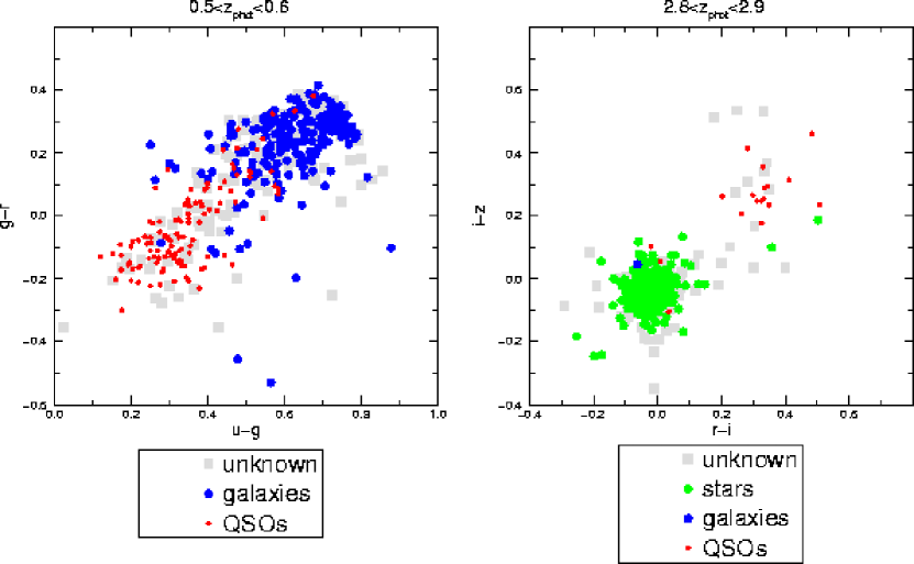
Figure 11: Two-dimensional projections of color-space, showing locations of various classes of objects in the FEDR. Left: FEDR objects with $0.5<z_{\mathrm{phot}}<0.6$, Right: FEDR objects with $2.8<z_{\mathrm{phot}}<2.9$. In both plots, gray squares are objects without spectra, red circles are quasars, green circles are stars, and blue circles are galaxies.

We can perhaps do even better by investigating whether non-quasars and quasars with similar $z_{\mathrm{phot}}$ can be separated by their colors. The two plots in Figure 11, which are two-dimensional projections of color-space, show the locations of various objects. Grey squares are of unknown type. Red, green, and blue circles are confirmed quasars, stars, and galaxies, respectively. The objects in the two plots of Figure 11 have photometric redshifts in the ranges 0.5-0.6 (left), and 2.8-2.9 (right). We see that most quasars and galaxies with photometric redshifts of 0.5-0.6 can be separated by $u-g$ and $g-r$, while most quasars and stars with photometric redshifts of 2.8-2.9 can be differentiated by $r-i$ and $i-z$. This allows us to retrieve most quasars with these photometric redshifts.

5.4 Objects of Unknown Type

Referring again to Figure 10, compare the $z_{\mathrm{phot}}$ distributions for all objects (grey bars) and objects with identifiable spectra (black bars). For $z_{\mathrm{phot}}<3$, the two distributions are roughly the same (except for overall normalization). However, for $z_{\mathrm{phot}}>3$, and especially for $z_{\mathrm{phot}}\sim 3.5$ and $z_{\mathrm{phot}}\sim 4.5$, there are many more objects without spectra than we might expect. This is because of the way the final quasar-selection algorithm was designed.

Previous versions of the selection algorithm missed many quasars with $z\sim 3.5$ and $z\sim 4.5$, because these lie in the same region of color-space as late-type stars. The final version was therefore designed to probe deeper into this region (Richards et al. 2002). Generally speaking, since the previous versions of the selection algorithm were used to make the EDR quasar catalog (for which spectra were taken), most of the objects in the FEDR that do not have spectra were only selected with the final selection algorithm. Thus, we find a striking abundance of objects with no spectra having $z_{\mathrm{phot}}>3$. Most of these are probably late-type stars that are included as contaminants in the SDSS’s attempt to be as complete as possible to bright $z>3$ quasars; many of these candidates are from a small number of data frames that have sub-standard photometry — causing stars within the stellar locus to scatter into the quasar distribution.

5.5 Objects with $0.8<z_{\mathrm{phot}}<2.2$ (“the Window”)

We now turn our attention to the objects whose photometric redshifts lie in the largely uncontaminated window between 0.8 and 2.2. These will be called Window objects.

There are 2459 objects in the Window; 1902 of them are confirmed quasars, while only 22 and 27 are confirmed stars and galaxies, respectively. The remaining 508 objects are of unknown type. If we assume that the distribution of unknown objects is the same as that of the known ones, then approximately 97.5% of the Window objects are quasars. If an object selected as a quasar-candidate by the selection algorithm has a $z_{\mathrm{phot}}$ in the Window, it is almost certainly a quasar.

The efficiency of the $z_{\mathrm{phot}}$ algorithm is also better in the Window. Out of the 1902 confirmed quasars in the Window, the number (percent) with photometric redshifts correct to within 0.1, 0.2, and 0.3 are: 1314 (69.1%), 1638 (86.1%), and 1746 (91.8%). Thus, 89.5% of the objects in the Window (that is, 91.8% of 97.5%) are quasars with photometric redshifts correct to within 0.3.

5.6 Color-space Cuts that Select Mostly Window Objects (“The Box”)

It is also of interest to determine regions of color space that yield higher than average quasar efficiencies (quasars : quasar candidates). Richards et al. (2004) describe the application of a complex algorithm to the SDSS-DR1 dataset; however, for many applications users may prefer a simpler method. As such, we define a region of color space that was designed to yield mostly Window objects such that one can dispense with the quasar-selection algorithm altogether and simply query the SDSS database for objects with colors in this region of color-space.

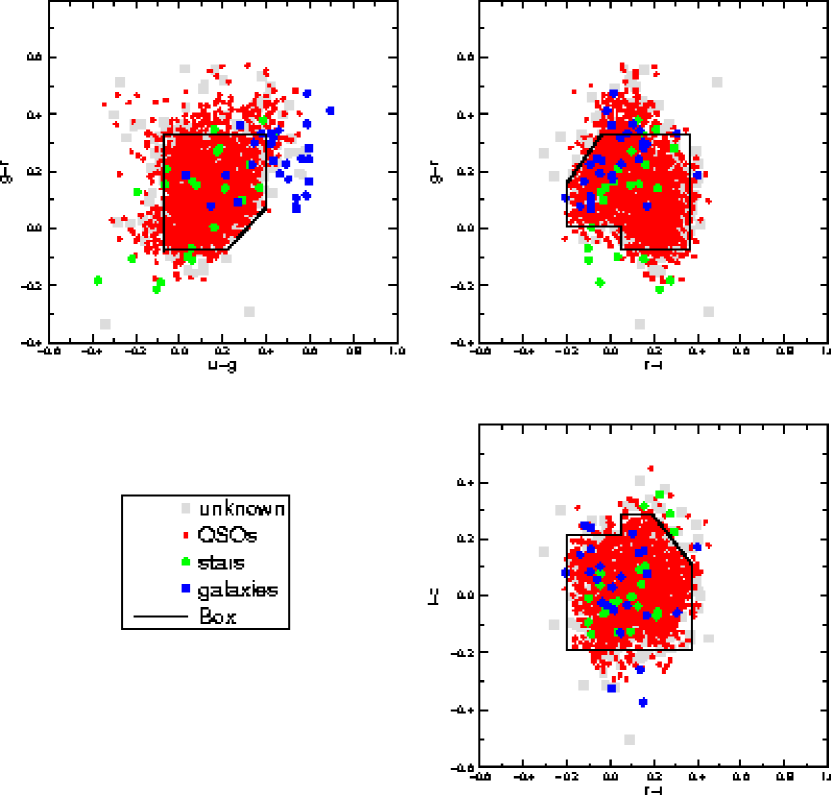
Figure 12: Two-dimensional projections of color-space, showing Box color-cuts (black lines), and the FEDR objects with $0.8<z_{\mathrm{phot}}<2.2$. Symbols are the same as in Figure 11.

Figure 12 shows a region of color-space which we call “the Box,” designed to include primarily Window objects. The Box is defined by the intersection of the following cuts in color-space:

$$\begin{array}[]{c}\begin{array}[]{rcccl}-0.07&<&u-g&<&0.40\\ \{0.01|-0.075\}&<&g-r&<&0.33\\ -0.20&<&r-i&<&0.37\\ -0.19&<&i-z&<&\{0.215|0.29\}\end{array}\\ \begin{array}[]{rcl}g-r&>&0.8333(u-g)-0.2583\\ g-r&<&1.0625(r-i)+0.3725\\ i-z&<&-0.9730(r-i)+0.4749\end{array}\end{array}$$

where $\{x|y\}$ is equal to $x$ if $r-i<0.05$ and $y$ if $r-i\geq 0.05$.

Of the 8740 objects in our sample, 1752 of them lie in the Box. 1578 of these are objects with $0.8<z_{\mathrm{phot}}<2.2$: 1256 confirmed quasars, 11 confirmed non-quasars, and 311 unknown objects. If we assume that the unknown objects contain the same fraction of quasars as the known ones, then 89.3% of the objects in the Box are quasars with $0.8<z_{\mathrm{phot}}<2.2$. Thus, the color-cuts we have chosen do succeed in selecting mostly Window quasars.

Of the 1256 Window quasars found in the Box, most have accurate photometric redshifts (as expected). There are 874 with $z_{\mathrm{phot}}$ accurate to within 0.1, 1086 to within 0.2, and 1159 to within 0.3. So if we apply the Box color-cuts to SDSS data, roughly 83% of them will be quasars with $z_{\mathrm{phot}}$ accurate to within 0.3. However, it must be kept in mind that although the Box is very efficient at picking out mostly Window quasars and little else, it by no means selects all of the Window quasars. Within our sample, there are 1902 confirmed quasars with $0.8<z_{\mathrm{phot}}<2.2$, whereas the Box contains only 1256, or 66%.

6 Summary

We have presented an updated version of the empirical quasar photo-$z$ algorithm originally presented by RW01. This improved version of the code yields redshifts for known quasars that are accurate to $\pm 0.3$ in redshift for 83% of quasars in the EDR quasar catalog. In addition, the algorithm returns accurate probabilities that these redshifts are within a given range — making it possible to better identify those 17% of quasars that have erroneous photo-$z$’s. We have further shown that it is possible to use the algorithm to identify non-quasars among quasar candidates and therefore to construct the most robust samples (in terms of quasar identification and photo-$z$ accuracy) among samples of unknown objects. Richards et al. (2004) discuss the application of this photo-$z$ algorithm to a sample of over 100,000 SDSS-DR1 quasar candidates. The efficiency of their selection algorithm combined with the accuracy of our photo-$z$ algorithm suggest that over 80,000 of these objects will be quasars with accurate photometric redshifts, demonstrating that it will be possible to construct a sample of hundreds of thousands of quasars by the end of the SDSS project. The C code for the algorithm described herein can be obtained by contacting either of the first two authors.

Figure 5: Distribution of $\Delta z=z_{\mathrm{spec}}-z_{\mathrm{phot}}$ for EDR quasars.

Figure 6: Distribution of photometric redshift range sizes for the EDR quasars.

Figure 7: Fraction of EDR quasars with confidence-level $P$ equal to prob for which $z_{\mathrm{spec}}$ is within the photo-$z$ range, where prob goes from 0 to 1 in bins of 0.05. Numbers denote total number of EDR quasars with confidence-level $P$.

References

- Abazajian, Adelman-McCarthy, Agüeros, Allam, Anderson, Annis, Bahcall, Baldry, Bastian, Berlind, Bernardi, Blanton, Blythe, Bochanski, Boroski, Brewington, Briggs, Brinkmann, Brunner, Budavári, Carey, Carr, Castander, Chiu, Collinge, Connolly, Covey, Csabai, Dalcanton, Dodelson, Doi, Dong, Eisenstein, Evans, Fan, Feldman, Finkbeiner, Friedman, Frieman, Fukugita, Gal, Gillespie, Glazebrook, Gonzalez, Gray, Grebel, Grodnicki, Gunn, Gurbani, Hall, Hao, Harbeck, Harris, Harris, Harvanek, Hawley, Heckman, Helmboldt, Hendry, Hennessy, Hindsley, Hogg, Holmgren, Holtzman, Homer, Hui, Ichikawa, Ichikawa, Inkmann, Ivezić, Jester, Johnston, Jordan, Jordan, Jorgensen, Jurić, Kauffmann, Kent, Kleinman, Knapp, Kniazev, Kron, Krzesiński, Kunszt, Kuropatkin, Lamb, Lampeitl, Laubscher, Lee, Leger, Li, Lidz, Lin, Loh, Long, Loveday, Lupton, Malik, Margon, McGehee, McKay, Meiksin, Miknaitis, Moorthy, Munn, Murphy, Nakajima, Narayanan, Nash, Neilsen, Newberg, Newman, Nichol, Nicinski, Nieto-Santisteban, Nitta, Odenkirchen, Okamura, Ostriker, Owen, Padmanabhan, Peoples, Pier, Pindor, Pope, Quinn, Rafikov, Raymond, Richards, Richmond, Rix, Rockosi, Schaye, Schlegel, Schneider, Schroeder, Scranton, Sekiguchi, Seljak, Sergey, Sesar, Sheldon, Shimasaku, Siegmund, Silvestri, Sinisgalli, Sirko, Smith, Smolčić, Snedden, Stebbins, Steinhardt, Stinson, Stoughton, Strateva, Strauss, SubbaRao, Szalay, Szapudi, Szkody, Tasca, Tegmark, Thakar, Tremonti, Tucker, Uomoto, Vanden Berk, Vandenberg, Vogeley, Voges, Vogt, Walkowicz, Weinberg, West, White, Wilhite, Willman, Xu, Yanny, Yarger, Yasuda, Yip, Yocum, York, Zakamska, Zehavi, Zheng, Zibetti, & Zucker (2003) Abazajian, K., Adelman-McCarthy, J. K., Agüeros, M. A., Allam, S. S., Anderson, S. F., Annis, J., Bahcall, N. A., Baldry, I. K., et al. 2003, AJ, 126, 2081
- Abazajian et al. (2004) Abazajian, K., Adelman-McCarthy, J. K., Agüeros, M. A., Allam, S. S., Anderson, K. S. J., Anderson, S. F., Annis, J., Bahcall, N. A., et al. 2004, AJ, 128, 502
- Benítez, Ford, Bouwens, Menanteau, Blakeslee, Gronwall, Illingworth, Meurer, Broadhurst, Clampin, Franx, Hartig, Magee, Sirianni, Ardila, Bartko, Brown, Burrows, Cheng, Cross, Feldman, Golimowski, Infante, Kimble, Krist, Lesser, Levay, Martel, Miley, Postman, Rosati, Sparks, Tran, Tsvetanov, White, & Zheng (2004) Benítez, N., Ford, H., Bouwens, R., Menanteau, F., Blakeslee, J., Gronwall, C., Illingworth, G., Meurer, G., et al. 2004, ApJS, 150, 1
- Blanton, Lin, Lupton, Maley, Young, Zehavi, & Loveday (2003) Blanton, M. R., Lin, H., Lupton, R. H., Maley, F. M., Young, N., Zehavi, I., & Loveday, J. 2003, AJ, 125, 2276
- Brunner, Connolly, Szalay, & Bershady (1997) Brunner, R. J., Connolly, A. J., Szalay, A. S., & Bershady, M. A. 1997, ApJ, 482, L21
- Budavári, Csabai, Szalay, Connolly, Szokoly, Vanden Berk, Richards, Weinstein, Schneider, Benítez, Brinkmann, Brunner, Hall, Hennessy, Ivezić, Kunszt, Munn, Nichol, Pier, & York (2001) Budavári, T., Csabai, I., Szalay, A. S., Connolly, A. J., Szokoly, G. P., Vanden Berk, D. E., Richards, G. T., Weinstein, M. A., et al. 2001, AJ, 122, 1163
- Connolly, Budavári, Szalay, Csabai, & Brunner (1999) Connolly, A. J., Budavári, T., Szalay, A. S., Csabai, I., & Brunner, R. J. 1999, in ASP Conf. Ser. 191: Photometric Redshifts and the Detection of High Redshift Galaxies, 13
- Cristiani, Alexander, Bauer, Brandt, Chatzichristou, Fontanot, Grazian, Koekemoer, Lucas, Monaco, Nonino, Padovani, Stern, Tozzi, Treister, Urry, & Vanzella (2004) Cristiani, S., Alexander, D. M., Bauer, F., Brandt, W. N., Chatzichristou, E. T., Fontanot, F., Grazian, A., Koekemoer, A., et al. 2004, ApJ, 600, L119
- Fukugita, Ichikawa, Gunn, Doi, Shimasaku, & Schneider (1996) Fukugita, M., Ichikawa, T., Gunn, J. E., Doi, M., Shimasaku, K., & Schneider, D. P. 1996, AJ, 111, 1748
- Gunn, Carr, Rockosi, Sekiguchi, Berry, Elms, de Haas, Ivezić , Knapp, Lupton, Pauls, Simcoe, Hirsch, Sanford, Wang, York, Harris, Annis, Bartozek, Boroski, Bakken, Haldeman, Kent, Holm, Holmgren, Petravick, Prosapio, Rechenmacher, Doi, Fukugita, Shimasaku, Okada, Hull, Siegmund, Mannery, Blouke, Heidtman, Schneider, Lucinio, & Brinkman (1998) Gunn, J. E., Carr, M., Rockosi, C., Sekiguchi, M., Berry, K., Elms, B., de Haas, E., Ivezić , Ž., et al. 1998, AJ, 116, 3040
- Hatziminaoglou, Mathez, & Pelló (2000) Hatziminaoglou, E., Mathez, G., & Pelló, R. 2000, A&A, 359, 9
- Hogg, Finkbeiner, Schlegel, & Gunn (2001) Hogg, D. W., Finkbeiner, D. P., Schlegel, D. J., & Gunn, J. E. 2001, AJ, 122, 2129
- Hopkins et al. (2004) Hopkins et al. 2004, AJ, accepted (astro-ph/0406293)
- Lupton, Gunn, Ivezić, Knapp, Kent, & Yasuda (2001) Lupton, R. H., Gunn, J. E., Ivezić, Z., Knapp, G. R., Kent, S., & Yasuda, N. 2001, in ASP Conf. Ser. 238: Astronomical Data Analysis Software and Systems X, Vol. 10, 269
- Lupton, Gunn, & Szalay (1999) Lupton, R. H., Gunn, J. E., & Szalay, A. S. 1999, AJ, 118, 1406
- Lynds (1971) Lynds, R. 1971, ApJ, 164, L73
- Mobasher, Idzi, Benítez, Cimatti, Cristiani, Daddi, Dahlen, Dickinson, Erben, Ferguson, Giavalisco, Grogin, Koekemoer, Mignoli, Moustakas, Nonino, Rosati, Schirmer, Stern, Vanzella, Wolf, & Zamorani (2004) Mobasher, B., Idzi, R., Benítez, N., Cimatti, A., Cristiani, S., Daddi, E., Dahlen, T., Dickinson, M., et al. 2004, ApJ, 600, L167
- Pier, Munn, Hindsley, Hennessy, Kent, Lupton, & Ivezić (2003) Pier, J. R., Munn, J. A., Hindsley, R. B., Hennessy, G. S., Kent, S. M., Lupton, R. H., & Ivezić, Ž. 2003, AJ, 125, 1559
- Richards, Fan, Newberg, Strauss, Vanden Berk, Schneider, Yanny, Boucher, Burles, Frieman, Gunn, Hall, Ivezić, Kent, Loveday, Lupton, Rockosi, Schlegel, Stoughton, SubbaRao, & York (2002) Richards, G. T., Fan, X., Newberg, H. J., Strauss, M. A., Vanden Berk, D. E., Schneider, D. P., Yanny, B., Boucher, A., et al. 2002, AJ, 123, 2945
- (20) Richards, G. T., Fan, X., Schneider, D. P., Vanden Berk, D. E., Strauss, M. A., York, D. G., Anderson, J. E., Anderson, S. F., et al. 2001a, AJ, 121, 2308
- Richards, Hall, Vanden Berk, Strauss, Schneider, Weinstein, Reichard, York, Knapp, Fan, Ivezić, Brinkmann, Budavári, Csabai, & Nichol (2003) Richards, G. T., Hall, P. B., Vanden Berk, D. E., Strauss, M. A., Schneider, D. P., Weinstein, M. A., Reichard, T. A., York, D. G., et al. 2003, AJ, 126, 1131
- (22) Richards, G. T., Weinstein, M. A., Schneider, D. P., Fan, X., Strauss, M. A., Vanden Berk, D. E., Annis, J., Burles, S., et al. 2001b, AJ, 122, 1151 (RW01)
- Richards et al. (2004) Richards et al. 2004, ApJS, submitted
- Schlegel, Finkbeiner, & Davis (1998) Schlegel, D. J., Finkbeiner, D. P., & Davis, M. 1998, ApJ, 500, 525
- Schneider, Fan, Hall, Jester, Richards, Stoughton, Strauss, SubbaRao, Vanden Berk, Anderson, Brandt, Gunn, Gray, Trump, Voges, Yanny, Bahcall, Blanton, Boroski, Brinkmann, Brunner, Burles, Castander, Doi, Eisenstein, Frieman, Fukugita, Heckman, Hennessy, Ivezić, Kent, Knapp, Lamb, Lee, Loveday, Lupton, Margon, Meiksin, Munn, Newberg, Nichol, Niederste-Ostholt, Pier, Richmond, Rockosi, Saxe, Schlegel, Szalay, Thakar, Uomoto, & York (2003) Schneider, D. P., Fan, X., Hall, P. B., Jester, S., Richards, G. T., Stoughton, C., Strauss, M. A., SubbaRao, M., et al. 2003, AJ, 126, 2579
- Schneider, Richards, Fan, Hall, Strauss, Vanden Berk, Gunn, Newberg, Reichard, Stoughton, Voges, Yanny, Anderson, Annis, Bahcall, Bauer, Bernardi, Blanton, Boroski, Brinkmann, Briggs, Brunner, Burles, Carey, Castander, Connolly, Csabai, Doi, Friedman, Frieman, Fukugita, Heckman, Hennessy, Hindsley, Hogg, Ivezić, Kent, Knapp, Kunzst, Lamb, Leger, Long, Loveday, Lupton, Margon, Meiksin, Merelli, Munn, Newcomb, Nichol, Owen, Pier, Pope, Rockosi, Saxe, Schlegel, Siegmund, Smee, Snir, SubbaRao, Szalay, Thakar, Uomoto, Waddell, & York (2002) Schneider, D. P., Richards, G. T., Fan, X., Hall, P. B., Strauss, M. A., Vanden Berk, D. E., Gunn, J. E., Newberg, H. J., et al. 2002, AJ, 123, 567
- Smith, Tucker, Kent, Richmond, Fukugita, Ichikawa, Ichikawa, Jorgensen, Uomoto, Gunn, Hamabe, Watanabe, Tolea, Henden, Annis, Pier, McKay, Brinkmann, Chen, Holtzman, Shimasaku, & York (2002) Smith, J. A., Tucker, D. L., Kent, S., Richmond, M. W., Fukugita, M., Ichikawa, T., Ichikawa, S., Jorgensen, A. M., et al. 2002, AJ, 123, 2121
- Stoughton, Lupton, Bernardi, Blanton, Burles, Castander, Connolly, Eisenstein, Frieman, Hennessy, Hindsley, Ivezić, Kent, Kunszt, Lee, Meiksin, Munn, Newberg, Nichol, Nicinski, Pier, Richards, Richmond, Schlegel, Smith, Strauss, SubbaRao, Szalay, Thakar, Tucker, Vanden Berk, Yanny, Adelman, Anderson, Anderson, Annis, Bahcall, Bakken, Bartelmann, Bastian, Bauer, Berman, Böhringer, Boroski, Bracker, Briegel, Briggs, Brinkmann, Brunner, Carey, Carr, Chen, Christian, Colestock, Crocker, Csabai, Czarapata, Dalcanton, Davidsen, Davis, Dehnen, Dodelson, Doi, Dombeck, Donahue, Ellman, Elms, Evans, Eyer, Fan, Federwitz, Friedman, Fukugita, Gal, Gillespie, Glazebrook, Gray, Grebel, Greenawalt, Greene, Gunn, de Haas, Haiman, Haldeman, Hall, Hamabe, Hansen, Harris, Harris, Harvanek, Hawley, Hayes, Heckman, Helmi, Henden, Hogan, Hogg, Holmgren, Holtzman, Huang, Hull, Ichikawa, Ichikawa, Johnston, Kauffmann, Kim, Kimball, Kinney, Klaene, Kleinman, Klypin, Knapp, Korienek, Krolik, Kron, Krzesiński, Lamb, Leger, Limmongkol, Lindenmeyer, Long, Loomis, Loveday, MacKinnon, Mannery, Mantsch, Margon, McGehee, McKay, McLean, Menou, Merelli, Mo, Monet, Nakamura, Narayanan, Nash, Neilsen, Newman, Nitta, Odenkirchen, Okada, Okamura, Ostriker, Owen, Pauls, Peoples, Peterson, Petravick, Pope, Pordes, Postman, Prosapio, Quinn, Rechenmacher, Rivetta, Rix, Rockosi, Rosner, Ruthmansdorfer, Sandford, Schneider, Scranton, Sekiguchi, Sergey, Sheth, Shimasaku, Smee, Snedden, Stebbins, Stubbs, Szapudi, Szkody, Szokoly, Tabachnik, Tsvetanov, Uomoto, Vogeley, Voges, Waddell, Walterbos, Wang, Watanabe, Weinberg, White, White, Wilhite, Wolfe, Yasuda, York, Zehavi, & Zheng (2002) Stoughton, C., Lupton, R. H., Bernardi, M., Blanton, M. R., Burles, S., Castander, F. J., Connolly, A. J., Eisenstein, D. J., et al. 2002, AJ, 123, 485
- Wolf, Meisenheimer, Röser, Beckwith, Chaffee, Fried, Hippelein, Huang, Kümmel, von Kuhlmann, Maier, Phleps, Rix, Thommes, & Thompson (2001) Wolf, C., Meisenheimer, K., Röser, H.-J., Beckwith, S. V. W., Chaffee, F. H., Fried, J., Hippelein, H., Huang, J.-S., et al. 2001, A&A, 365, 681
- Wolf, Wisotzki, Borch, Dye, Kleinheinrich, & Meisenheimer (2003) Wolf, C., Wisotzki, L., Borch, A., Dye, S., Kleinheinrich, M., & Meisenheimer, K. 2003, A&A, 408, 499
- York, Adelman, Anderson, Anderson, Annis, Bahcall, Bakken, Barkhouser, Bastian, Berman, Boroski, Bracker, Briegel, Briggs, Brinkmann, Brunner, Burles, Carey, Carr, Castander, Chen, Colestock, Connolly, Crocker, Csabai, Czarapata, Davis, Doi, Dombeck, Eisenstein, Ellman, Elms, Evans, Fan, Federwitz, Fiscelli, Friedman, Frieman, Fukugita, Gillespie, Gunn, Gurbani, de Haas, Haldeman, Harris, Hayes, Heckman, Hennessy, Hindsley, Holm, Holmgren, Huang, Hull, Husby, Ichikawa, Ichikawa, Ivezić, Kent, Kim, Kinney, Klaene, Kleinman, Kleinman, Knapp, Korienek, Kron, Kunszt, Lamb, Lee, Leger, Limmongkol, Lindenmeyer, Long, Loomis, Loveday, Lucinio, Lupton, MacKinnon, Mannery, Mantsch, Margon, McGehee, McKay, Meiksin, Merelli, Monet, Munn, Narayanan, Nash, Neilsen, Neswold, Newberg, Nichol, Nicinski, Nonino, Okada, Okamura, Ostriker, Owen, Pauls, Peoples, Peterson, Petravick, Pier, Pope, Pordes, Prosapio, Rechenmacher, Quinn, Richards, Richmond, Rivetta, Rockosi, Ruthmansdorfer, Sandford, Schlegel, Schneider, Sekiguchi, Sergey, Shimasaku, Siegmund, Smee, Smith, Snedden, Stone, Stoughton, Strauss, Stubbs, SubbaRao, Szalay, Szapudi, Szokoly, Thakar, Tremonti, Tucker, Uomoto, Vanden Berk, Vogeley, Waddell, Wang, Watanabe, Weinberg, Yanny, & Yasuda (2000) York, D. G., Adelman, J., Anderson, J. E., Anderson, S. F., Annis, J., Bahcall, N. A., Bakken, J. A., Barkhouser, R., et al. 2000, AJ, 120, 1579