Supersonic Motions of Galaxies in Clusters

Abstract

We study motions of galaxies in galaxy clusters formed in the concordance $\Lambda$CDM cosmology. We use high-resolution cosmological simulations that follow dynamics of dark matter and gas and include various physical processes critical for galaxy formation: gas cooling, heating and star formation. Analysing motions of galaxies and the properties of intracluster gas in the sample of eight simulated clusters at $z=0$, we study velocity dispersion profiles of the dark matter, gas, and galaxies. We measure the mean velocity of galaxy motions and gas sound speed as a function of radius and calculate the average Mach number of galaxy motions. The simulations show that galaxies, on average, move supersonically with the average Mach number of $\approx 1.4$, approximately independent of the cluster-centric radius. The supersonic motions of galaxies may potentially provide an important source of heating for the intracluster gas by driving weak shocks and via dynamical friction, although these heating processes appear to be inefficient in our simulations. We also find that galaxies move slightly faster than the dark matter particles. The magnitude of the velocity bias, $b_{v}\approx 1.1$, is, however, smaller than the bias estimated for subhalos in dissipationless simulations. Interestingly, we find velocity bias in the tangential component of the velocity dispersion, but not in the radial component. Finally, we find significant random bulk motions of gas. The typical gas velocities are of order $\approx 20-30\%$ of the gas sound speed. These random motions provide about $10\%$ of the total pressure support in our simulated clusters. The non-thermal pressure support, if neglected, will bias measurements of the total mass in the hydrostatic analyses of the X-ray cluster observations.

1 Introduction

Clusters of galaxies are powerful probes of both the overall cosmic evolution and evolution of galaxies in dense environments. Most of the cluster baryons are in the form of hot diffuse plasma and stars in galaxies, with a fraction of $\sim 10-50\%$ of stars in the intracluster medium. Interaction between galaxies and the hot intracluster gas is thought to be important in shaping properties of both components. The compression of the interstellar medium (ISM) of an accreted galaxy and cluster tidal forces can lead to a starformation burst (Dressler & Gunn, 1983; Gavazzi et al., 1995; Rose et al., 2001; Koopmann & Kenney, 2004; Sakai et al., 2002) or active galactic nuclei (AGN) activity (e.g., Miller & Owen, 2003) and morphological transformation (Moore et al., 1996; Koopmann & Kenney, 2004; Gnedin, 2003). The subsequent removal of the ISM by ram pressure stripping (Gunn & Gott, 1972) and other processes (e.g., Nulsen, 1982) can suppress starformation, dramatically affecting properties of cluster galaxy population (e.g., Quilis et al., 2000; Schulz & Struck, 2001; Vollmer et al., 2001; Vollmer, 2003). Galaxies, in turn, may heat the intracluster medium (ICM) via supernova or AGN feedback and enrich it with heavy elements (e.g., Kaiser, 1991; Metzler & Evrard, 1994; Valageas & Silk, 1999; Churazov et al., 2002; Fabian et al., 2002; Scannapieco & Oh, 2004; Voit & Ponman, 2003; Ruszkowski et al., 2004). Galaxies can stir the surrounding gas as they move through the ICM driving turbulent flows and mixing the gas. The kinetic energy of galaxy motions can also be an important source of the ICM heating (e.g., Miller, 1986; El-Zant, Kim & Kamionkowski, 2004).

In the currently favoured Cold Dark Matter (CDM) model of structure formation, galaxies form in the extended dark matter halos as gas cools and condenses in the centre. After a galaxy is accreted by a cluster, the tidal forces can quickly strip the outer loosely bound regions of DM halos and can lead to a total disruption of the halo and, possibly, the stellar system. The dynamical evolution of galaxy-size dark matter halos in groups and clusters (often called the subhalos) has been the subject of many recent studies, which used a new generation of high-resolution dissipationless simulations not affected by the “overmerging” problem (Ghigna et al., 1998; Tormen et al., 1998; Klypin et al., 1999; Colín et al., 1999; Okamoto & Habe, 1999; Colín et al., 2000; Ghigna et al., 2000; De Lucia et al., 2004; Kravtsov et al., 2004; Desai et al., 2004; Diemand et al., 2004; Gao et al., 2004; Reed et al., 2004).

These studies find that abundance of subhalos is in reasonable agreement with the observed abundance of cluster galaxies (Moore et al., 1999; Kravtsov et al., 2004; Desai et al., 2004, see, however, Diemand et al. 2004 and Gao et al. 2004), although there are suggestive differences in the radial distribution (Diemand et al., 2004; Gao et al., 2004; Nagai & Kravtsov, 2005) and circular velocity functions (Desai et al., 2004). Interestingly, velocity dispersion of subhalos is larger than that of dark matter by a factor up to $\approx 1.4$ in the inner regions of clusters (Colín et al., 2000; Ghigna et al., 2000; Diemand et al., 2004; Gao et al., 2004), implying that dynamical estimates of cluster masses using galaxy velocity dispersion may be biased. However, applying results of dissipationless simulations to the properties of cluster galaxies is subject to many caveats. Gas cooling during galaxy formation increases central density of DM halos (e.g., Blumenthal et al., 1986; Gnedin et al., 2004), making them more resistant to tidal disruption. In the inner regions of galaxies stellar density is typically considerably higher than that of DM and the luminous component can survive the tidal forces even if the surrounding DM halo is completely disrupted (e.g., Gao et al., 2004). It is therefore critical to study the properties of cluster galaxies forming in self-consistent cosmological simulations.

Although a number of studies during the last decade used gasdynamics cosmological simulations with cooling to study spatial distribution of galaxies (e.g., Katz et al., 1992; Pearce et al., 1999; Yoshikawa et al., 2001; Weinberg et al., 2004; Zheng et al., 2004), only a few analyses directly addressed the motions of galaxies in cluster halos. Frenk et al. (1996) used simulations with cooling and starformation to study distribution and dynamics of galaxies in clusters. They found that the velocity dispersion of massive galaxies in the simulations is lower than that of the DM by $\sim 20-30\%$, which they attributed to the orbital energy loss due to dynamical friction. More recently, Berlind et al. (2003) analysed mean motions of galaxies, identified as dense baryonic clumps, in halos of different masses in SPH simulations. These authors find that galaxies selected to have baryonic masses above a certain threshold move slower than DM in galaxy and group-size halos, the bias that disappears for more massive cluster-size halos.

In this paper we present analysis of a sample of eight galaxy clusters formed in high-resolution cosmological simulations of the $\Lambda$CDM model. The simulations follow dynamics of DM and gas and include relevant cooling and heating processes and star formation. We use a combined sample of cluster galaxies, constructed using the friends-of-friends (FoF) algorithm, to study the average statistical properties of galaxy motions and compare them to the corresponding statistics calculated for the DM and intracluster gas. A complementary study of the radial distribution of galaxies in these simulations is presented in Nagai & Kravtsov (2005).

The paper is organised as follows. In § 2 we introduce the simulation and describe the cluster sample which the subsequent analysis is based on. In § 3 we describe details of the galaxy finding algorithm and present analysis of the overall spatial and velocity distributions of galaxies. In § 4 we study the radial profiles of the velocity dispersion and velocity anisotropy for the DM, gas, and galaxies. The radial dependence of the average Mach number of galaxy motions in simulated clusters is presented in § 4.3. Finally, in § 5 we summarise our main results and conclusions.

2 Simulated cluster sample

2.1 Simulations

In this study, we analyse high-resolution cosmological simulations of eight group and cluster-size systems formed in the “concordance” flat $\Lambda$CDM model: $\Omega_{\rm m}=1-\Omega_{\Lambda}=0.3$, $\Omega_{\rm b}=0.021h^{-2}$, $h=0.7$ and $\sigma_{8}=0.9$, where the Hubble constant is defined as $100h{\ \rm km\ s^{-1}\ Mpc^{-1}}$, and $\sigma_{8}$ is the power spectrum normalisation on $8h^{-1}$ Mpc scale. The simulations were done with the Adaptive Refinement Tree (ART) $N$-body$+$gasdynamics code (Kravtsov, Klypin & Khokhlov, 1997; Kravtsov, 1999; Kravtsov, Klypin & Hoffman, 2002), a Eulerian code that uses the adaptive refinement in space and time and (non-adaptive) refinement in mass (Klypin et al., 2001) to reach the high dynamic range required to resolve cores of halos formed in self-consistent cosmological simulations.

To set up initial conditions we first ran a low resolution simulation of an $80h^{-1}$ Mpc box and selected eight clusters. The virial masses of clusters we selected range from $\approx 7\times 10^{13}$ to $3\times 10^{14}h^{-1}{\ \rm M_{\odot}}$. The perturbation modes in the lagrangian region corresponding to the sphere of five virial radii around each cluster at $z=0$ have then been re-sampled at the initial redshift, $z_{i}=49$, retaining the previous large-scale waves intact but including additional small-scale waves, as described by Klypin et al. (2001).

High-resolution simulations were run using 128³ uniform grid and 8 levels of mesh refinement in the computational box of $80h^{-1}$ Mpc, which corresponds to the dynamic range of $128\times 2^{8}=32768$ and peak formal resolution of $80/32,768\approx 2.44h^{-1}\ \rm kpc$, corresponding to the actual resolution of $\approx 2\times 2.44\approx 5h^{-1}\ \rm kpc$. Only the region of $\sim 10h^{-1}\ \rm Mpc$ around the cluster was adaptively refined, the rest of the volume was followed on the uniform $128^{3}$ grid. The dark matter particle mass in the region around the cluster was $2.7\times 10^{8}h^{-1}{\rm\ M_{\odot}}$, while other regions were simulated with lower mass resolution.

As the zeroth-level fixed grid consisted of only $128^{3}$ cells, we started the simulation already pre-refined to the 2nd level ($l=0,1,2$) in the high-resolution lagrangian regions of clusters. This is done to ensure that the cell size is equal to the mean interparticle separation and all fluctuations present in the initial conditions are evolved properly. During the simulation, the refinements were allowed to the maximum $l=8$ level and refinement criteria were based on the local mass of DM and gas in each cell. The logic is to keep the mass per cell approximately constant so that the refinements are introduced to follow the collapse of matter in a quasi-lagrangian fashion. For the DM, we refine the cell if it contains more than two dark matter particles of the highest mass resolution specie. For gas, we allow the mesh refinement, if the cell contains gas mass larger than four times the DM particle mass scaled by the baryon fraction. In other words, the mesh is refined if the cell contains the DM mass larger than $5.42\times 10^{8}h^{-1}\ {\rm M_{\odot}}$ $=2(1-f_{b})m_{p}$ or the gas mass larger than $1.81\times 10^{8}h^{-1}\ {\rm M_{\odot}}$ $=4f_{b}m_{p}$, where $m_{p}=3.16\times 10^{8}h^{-1}\ {\rm M_{\odot}}$ and $f_{b}=\Omega_{\rm b}/\Omega_{\rm m}$ = 0.1429. We analyse clusters at the present-day epoch as well as their progenitors at higher redshifts.

Simulations included gasdynamics and several physical processes critical to various aspects of galaxy formation: star formation, metal enrichment and thermal feedback due to the supernovae type II and type Ia, self-consistent advection of metals, metallicity-dependent radiative cooling and UV heating due to cosmological ionising background (Haardt & Madau, 1996). The cooling and heating rates take into account Compton heating/cooling of plasma, UV heating, atomic and molecular cooling and are tabulated for the temperature range $10^{2}<T<10^{9}$ K and a grid of metallicities, and UV intensities using the Cloudy code (ver. 96b4, Ferland et al., 1998). The Cloudy cooling and heating rates take into account metallicity of the gas, which is calculated self-consistently in the simulation, so that the local cooling rates depend on the local metallicity of the gas.

Star formation in these simulations was done using the observationally-motivated recipe (e.g., Kennicutt, 1998): $\dot{\rho}_{\ast}=\rho_{\rm gas}^{1.5}/t_{\ast}$, with $t_{\ast}=4\times 10^{9}$ yrs. Stars are allowed to form in regions with temperature $T<2\times 10^{4}$ K and gas density $n>0.1\ \rm cm^{-3}$. No other criteria (like the collapse condition $\nabla\cdot{\bf v}<0$) were used. Algorithmically, star formation events are assumed to occur once every global time step $\Delta t_{0}\sim 10^{7}$ yrs, the value close to the observed timescales (e.g., Hartmann, 2002). Collisionless stellar particles with mass $m_{\ast}=\dot{\rho}_{\ast}\Delta t_{0}$ are formed in every unrefined mesh cell that satisfies criteria for star formation during star formation events. The mass of stellar particles is restricted to be larger than $\min(5\times 10^{7}h^{-1}{\ \rm M_{\odot}},2/3\times m_{\rm gas})$, where $m_{\rm gas}$ is gas mass in the star forming cell. This is done in order to keep the number of stellar particles computationally tractable, while avoiding sudden dramatic decrease of the local gas density. In the simulations analysed here, the masses of stellar particles formed by this algorithm range from $\approx 10^{5}$ to $7\times 10^{8}h^{-1}{\ \rm M_{\odot}}$.

Once formed, each stellar particle is treated as a single-age stellar population and its feedback on the surrounding gas is implemented accordingly. The feedback here is meant in a broad sense and includes injection of energy and heavy elements (metals) via stellar winds and supernovae and secular mass loss. Specifically, in the simulations analysed here, we assumed that stellar initial mass function (IMF) is described by the Miller & Scalo (1979) functional form with stellar masses in the range $0.1-100\ \rm M_{\odot}$. All stars more massive than $M_{\ast}>8{\ \rm M_{\odot}}$ deposit $2\times 10^{51}$ ergs of thermal energy in their parent cell and fraction $f_{\rm Z}={\rm min}(0.2,0.01M_{\ast}-0.06)$ of their mass as metals, which crudely approximates the results of Woosley & Weaver (1995). In addition, the stellar particles return a fraction of their mass and metals to the surrounding gas at a secular rate $\dot{m}_{\rm loss}=m_{\ast}\,\,C_{0}(t-t_{\rm birth}+T_{0})^{-1}$ with $C_{0}=0.05$ and $T_{0}=5$ Myr (Jungwiert et al., 2001). The code also accounts for SNIa feedback assuming a rate that slowly increases with time and broadly peaks at the population age of 1 Gyr. We assume that a fraction of $1.5\times 10^{-2}$ of mass in stars between 3 and $8\ \rm M_{\odot}$ explodes as SNIa over the entire population history and each SNIa dumps $2\times 10^{51}$ ergs of thermal energy and ejects $1.3\ \rm M_{\odot}$ of metals into parent cell. For the assumed IMF, 75 SNII (instantly) and 11 SNIa (over several billion years) are produced by a $10^{4}\ \rm M_{\odot}$ stellar particle.

2.2 Cluster sample

Table 1 lists properties of the eight clusters used in this study. The mass of each cluster is defined within the radius enclosing the cumulative density of $500\rho_{crit}$, where $\rho_{crit}$ is the critical density of the universe. This choice of overdensity is motivated by the fact that clusters are on average more relaxed in their inner regions (Evrard, Metzler & Navarro, 1996). Additionally, most of the X-ray radiation comes from region within $r_{500}$ so this radius is preferred in X-ray observations. In the following we use the radius $r_{500}$, mass $M_{500}\equiv M(<r_{500})$, and circular velocity at $r_{500}$, $v_{500}\equiv\sqrt{GM_{500}/r_{500}}$, to normalise the physical cluster-centric radii, masses, and velocities. We will use the normalised quantities to obtain statistics averaged over all simulated clusters.

id	$r_{500}$	$v_{500}$	$m_{dark}$	$m_{gas}$	$m_{star}$
1	606	963	1.111	0.105	0.091
2	661	1047	1.431	0.137	0.115
3	621	988	1.202	0.120	0.085
4	520	830	0.706	0.074	0.054
5	486	771	0.570	0.043	0.059
6	535	851	0.763	0.078	0.061
7	506	806	0.648	0.061	0.055
8	465	743	0.509	0.044	0.045
mean	550	875	0.867	0.083	0.070

Table 1: Characteristic properties of the clusters. Column description: (1) the identification number of each cluster; (2) the radius $r_{500}$ enclosing overdensity of $500\times\rho_{crit}$ in ${\,h^{-1}\rm kpc}$; (3) circular velocity at $r_{500}$: $v_{500}\equiv\sqrt{GM_{500}/r_{500}}$ in ${\rm km/s}$; (4-6) the mass of dark matter, gas, and stars within $r_{500}$ in units of $10^{14}{\,h^{-1}\rm M}_{\odot}$. The last row shows the mean values averaged over all eight clusters.

3 Galaxy sample

3.1 Galaxy identification

We use the friends-of-friends (FoF) algorithm (e.g., Einasto et al., 1984) to identify galaxies in the simulations. The galaxies are defined as groups of stellar particles linked by the FoF with a certain linking length. We should note that the use of the FoF algorithm in dense environments can lead to misidentification of systems in two ways. First, distinct objects connected by an accidental bridge of small number of particles can be identified by the algorithm as a single object. Second, the algorithm can identify an unbound group of particles which does not correspond to a real physical system. To minimise such problems, we adopt a two-step clustering analysis.

In the first step, we identify groups with the FoF linking length of $ll=5{\,h^{-1}\rm kpc}$. This empirical value is similar to the typical sizes of galaxies and is well below the average distance between galaxies in a cluster. It is also close to the peak spatial resolution in the simulation. In the second step, we consider identified groups of more than $100$ stellar particles and apply the FoF analysis with a smaller linking length of $ll=2{\,h^{-1}\rm kpc}$ only to particles belonging to these groups. For our analysis, we then consider only identified stellar particle groups (galaxies) with more than $50$ particles linked with $ll=2{\,h^{-1}\rm kpc}$.

Figure 1: The data points represent the properties of all the galaxies found in the eight simulated clusters at z=0 using the approach described in section 3.1. The upper panel compares the stellar mass content within spheres of radius $50{\,h^{-1}\rm kpc}$ and $75{\,h^{-1}\rm kpc}$. The data points which coincide with the dashed diagonal belong to galaxies which contain all of their stellar mass within a radius of $50{\,h^{-1}\rm kpc}$. The middle panel shows a comparison between the masses ${\rm M}_{ll}$ obtained by FOF with $ll=5\rm{kpc}/h$ and the masses within a sphere of radius $50{\,h^{-1}\rm kpc}$. Points located on the dashed diagonal represent $100\%$ consistency of the masses obtained by the FoF approach and the masses gathered within a sphere of $50{\,h^{-1}\rm kpc}$. The lower panel depicts the relation between galaxy mass and distance to the cluster centre. Where the distance of each galaxy is scaled by $r_{500}$ (see Table 1) of the hosting cluster.

Figure 1 compares the stellar masses, $M_{50}$ and $M_{75}$, within the spheres of $r_{50}=50{\,h^{-1}\rm kpc}$ and $r_{75}=75{\,h^{-1}\rm kpc}$ radii around the identified stellar groups in all eight clusters. The upper panel of figure 1 shows that the dominant fraction of stellar mass resides within a radius of $50{\,h^{-1}\rm kpc}$. In a few cases the $M_{75}$ substantially exceeds $M_{50}$. These rare cases correspond to close encounters between galaxies resulting in a significant overlap of their stars. This occurs most often when a small galaxy passes near the central cluster galaxy. The comparison of the FOF masses $M_{ll}$ and $M_{50}$ shows that the FoF with $ll=5{\,h^{-1}\rm kpc}$ correctly links all of the stellar mass in galaxies. The small deviation from the $M_{ll}=M_{50}$ line at low masses is due to the contamination by the background particles. The background of intracluster stars and stars associated with the central galaxies at small masses provides a small contribution to the mass within $50{\,h^{-1}\rm kpc}$ for small sized objects. The contribution is evidently small however for our purposes and we did not attempt to correct for it.

The lower panel of figure 1 shows the cluster-centric distance of the individual galaxies (scaled by the $r_{500}$ of the corresponding cluster) versus ${\rm M}_{50}$. There is a small deficiency of low mass ($M_{50}\lesssim 5\times 10^{9}{\,h^{-1}\rm M}_{\odot}$) and high mass ($M_{50}\gtrsim 2\times 10^{11}{\,h^{-1}\rm M}_{\odot}$) galaxies at small distances. The small mass galaxies are likely affected by the limited numerical resolution and tidal force of the cluster which leads to the tidal mass and possibly complete disruption. The minimum particle number limit we imposed can then exclude such objects. At large masses, the deficiency is likely due to the efficient merging via dynamical friction.

3.2 Galaxy number density profile

In our analysis below we use the average number density profile of the compiled galaxy sample. The profile is shown in figure 2. For comparison we also show the average DM and gas density profiles. The profiles are calculated by averaging profiles of individual clusters with radii normalised to $r_{500}$ and densities normalised to the mean densities within $r_{500}$.

Figure 2: Average density profiles of galaxy number density (diamond symbols) and density of dark matter (solid line) and gas (dotted line). The error bars for galaxy number density indicate the $1\sigma$ confidence interval. The dashed line is a fit of the analytic NFW profile (eq. [1]). The relative normalisation of the DM, gas, and galaxy profiles is arbitrary.

We fit the galaxy number density profile with the analytic NFW profile (Navarro et al., 1996, 1997):

$$n_{\rm gal}(r)={n_{0}\over(r/r_{s})(1+r/r_{s})^{2}}\ .$$ (1)

The galaxy profile is well described by the NFW profile at $r/r_{500}\gtrsim 0.5$ but is flatter than the profile of DM at smaller radii. The difference may be caused by tidal mass loss and disruption experienced by galaxies in the core of the cluster. The difference is rather small, however. The overall galaxy distribution is rather similar to that of dark matter at the radii we reliably probe. The detailed analysis of the galaxy number density profiles in these simulations and comparisons with observations are presented in Nagai & Kravtsov (2005).

3.3 Velocity distribution

Before we proceed to the analysis of average galaxy motions, it is important to consider velocity distribution of cluster galaxies. If the velocity distribution follows the Maxwell-Boltzmann distribution both the velocity dispersion and the mean velocity are meaningful and are connected by the well-defined relation. Figure 3 shows the velocity distribution of the compiled galaxy sample and the Maxwell-Boltzmann distribution. The distribution was calculated using galaxy velocities normalised to the circular velocities, $v_{500}$, of their host clusters. The Maxwell-Boltzmann distribution shown in the figure is given by

$$f(v)=N\sqrt{{2\over\pi}}\left({3\over\sigma^{2}_{\rm 3D}}\right)^{3/2}v^{2}\exp\left(-{3v^{2}\over 2\sigma^{2}_{\rm 3D}}\right)\ ,$$ (2)

where $\sigma_{\rm 3D}$ is the three dimensional velocity dispersion. Here $\sigma_{\rm 3D}$ is calculated using normalised galaxy velocities, $v/v_{500}$. Note that the dashed line in the figure is not a fit: it is the distribution given above calculated with the galaxy velocity dispersion measured for the galaxies in our compiled sample.

Figure 3: The normalised velocity distribution of the compiled galaxy sample (diamonds) and the Maxwell-Boltzmann velocity distribution (dashed line for all galaxies within $r<5r_{500}$). The error bars for galaxy distribution indicate the $1\sigma$ confidence interval. Note that the Maxwell-Boltzmann distribution is not a fit. It is calculated using the measured velocity dispersion of the galaxy sample.

The figure shows that the velocity distribution of the galaxy sample is well described by the Maxwell-Boltzmann distribution. One can therefore derive the mean velocity of the galaxies from their three dimensional velocity dispersion. We will use this relation below to compute the mean velocity of galaxy motions.

4 Galaxy Motions

In this section, we analyse the motions of galaxies in the simulated clusters. The analysis consists of three parts. First, we measure the mean radial velocity, $v_{r}$, the three dimensional velocity dispersion, $\sigma_{\rm 3D}$, and its radial and tangential components, $\sigma_{r}$ and $\sigma_{t}$, of dark matter, gas and galaxies directly from the simulations. The errors for the galaxy measurements are computed using the $\sigma^{2}$ as the basic values, for the 3D distribution as well as for the radial and tangential components. Then the 67% confidence interval is computed and by means of error regression transformed to the actually shown error range of the various $\sigma$ distributions (compare to Colín et al. 2000). Using the radial profiles of $\sigma_{r}$ and $\sigma_{t}$ we can then compute the radial dependence of the velocity anisotropy parameter, $\beta$ (see eq. [3]). We also measure the sound speed $c_{s}$ of gas directly from the simulation. Second, we perform analyses using the equilibrium equations to model different components of galaxy clusters: the Jeans equation for galaxies and the hydrostatic equilibrium equation for the intracluster gas. Using the above measurements as inputs, we use the Jeans equations to solve for the radial velocity dispersion profile of galaxies. Similarly, we apply the hydrostatic equilibrium equation to solve for the sound speed of gas. These results are then compared to the direct measurements from the simulations to assess the validity of the equilibrium equations in modelling kinematics of galaxies and gas. Third, we study the average Mach number of galaxy motions as a function of cluster-centric radius. As we show below, we find that galaxies on average move supersonically with the average Mach number of $1.3-1.4$ throughout the cluster volume.

4.1 Velocity dispersion, anisotropy, and sound speed profiles

We measure the mean radial velocity, $v_{r}$, and the three dimensional velocity dispersion profile, $\sigma_{\rm 3D}(r)$ (and its radial and tangential components, $\sigma_{r}(r)$ and $\sigma_{t}(r)$) for dark matter, gas and galaxies in radial bins centered on the minimum of cluster potential after subtracting the peculiar velocity of the cluster. The peculiar velocity of the cluster is calculated as the mass-weighted bulk velocity of dark matter enclosed within $r_{500}$. We scale these measurements by the circular velocity $v_{500}$ measured at $r_{500}$ of each cluster. After re-scaling, we compute the average profiles for the sample of eight simulated clusters at $z=0$.

The upper four panels of figure 5 show the profiles measured in the simulations. The net radial velocity is small throughout the cluster for both the dark matter and gas, except in the cluster core where there is a small net inward motion. Galaxies, on the other hand, show some net radial velocity in some radial bins. However, the magnitude of the velocity, $\sim 0.2v_{500}$, is small compared to the velocity dispersion of the galaxies. Note that we find considerably smaller net radial velocity if we analyse each cluster at an epoch near $z=0$, when it appears to be most relaxed. This indicates that the net radial velocity seen in the $z=0$ sample is likely due to incompletely erased galaxy groups within the clusters.

We find that the three dimensional velocity dispersion of galaxies is biased with respect to that of dark matter. In other words, galaxies, on average, move faster than the average speed of dark matter particles in clusters. The velocity bias, $b_{v}=\sigma_{\rm gal}/\sigma_{\rm dm}$, is $b_{v}\approx 1.1$ within the virial radius and disappears outside the virial radius of the cluster. Note that the velocity bias we find for the stellar systems is smaller than the velocity bias found for subhalos in dissipationless simulations, $b_{v}\sim 1.2-1.4$ (Colín et al., 2000; Ghigna et al., 2000; Diemand et al., 2004; Gao et al., 2004). Interestingly, we find that the velocity bias comes entirely from the tangential component of the velocity dispersion. As can be seen in figure 5, the radial velocity dispersion of galaxies and dark matter match well.

Figure 5 also shows that gas within the virial radius is not at rest but has non-zero velocity dispersion. We find that the 3D velocity dispersion of gas is approximately constant at $\sigma_{\rm gas}\approx 0.4-0.5v_{500}$. In the inner regions of clusters gas moves with typical velocity of $\sigma_{\rm gas}/\sqrt{3}\sim 0.2-0.3c_{s}$, but gas velocity dispersion becomes $\sim 0.5c_{s}$ outside the virial radius reflecting the increasing strength of the infall motions and lesser degree of relaxation (see also Nagai, Kravtsov & Kosowsky, 2003; Sunyaev, Norman & Bryan, 2003). Note that these random velocities of gas contribute to the pressure support within clusters, in addition to the support from thermal pressure.

The bottom-left panel of the figure 5 shows the radial profile of the velocity anisotropy parameter,

$$\beta(r)=1-{\sigma^{2}_{t}(r)\over 2\sigma^{2}_{r}(r)}$$ (3)

(see, e.g., Binney & Tremaine 1987). The figure shows that both the dark matter and gas tend to have a slight radial anisotropy. The anisotropy is nearly constant in magnitude: $\beta\approx 0.2$ for dark matter (cp. Hoeft et al. 2004) and $\beta\approx 0.4$ for gas. Note, however, the velocity anisotropy of gas drops within $\beta\approx 0.2$ in the centre. For galaxies, we find similar values of $\beta$ on the outskirts of clusters. However, the value of $\beta$ decreases gradually and reaches zero at $r\lesssim 0.5r_{500}$. A fit to the actual measurements in simulations using the fitting formula of Colín et al. (2000),

$$\beta=\beta_{m}{4r\over r^{2}+4}+\beta_{0}\ ,$$ (4)

gives best fit parameters of $(\beta_{m},\beta_{0})=(0.76,-0.39)$. This fit is shown as a dashed line in figure 5. It describes the values measured in simulations quite well. Our best fit value of $\beta_{0}$ is systematically smaller than the value found by Colín et al. (2000) in dissipationless simulations. This indicates that velocities of galaxies in our simulations have more enhanced tangential velocity dispersion compared to the subhalos in dissipationless simulations.

The bottom-right panel in the figure 5 shows the average sound speed of intracluster gas. We compute this quantity in two ways. First, we measure the average sound speed of gas in the vicinity of galaxies, as sketched in the figure 4, and average over the measurements of all galaxies in each radial bin. Alternatively, we measure the average sound speed of gas by simply computing the average of the sound speeds measured in individual mesh cells in each bin. The figure shows that the average sound speeds calculated in these two ways agree well. Note that the sound speed of gas is not constant but increases monotonically toward the cluster centre.

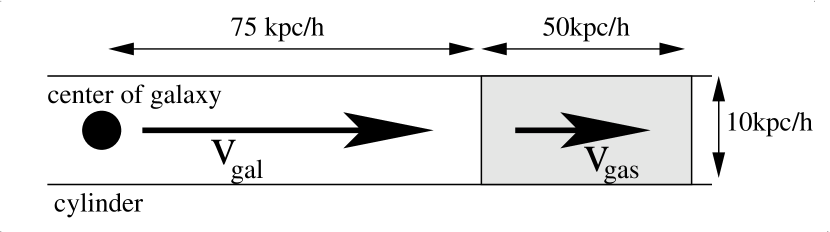
Figure 4: The sketch illustrates the measurements of the sound speed of gas in the vicinity of galaxies. We first identify the centre of the galaxy (marked as the solid circle) and draw a cylinder with the diameter of $10h^{-1}{\rm kpc}$ aligned parallel to the direction of galaxy motion. We then measure the average sound speed of gas in a segment of the cylinder with the size of $50h^{-1}{\rm kpc}$ located $75h^{-1}{\rm kpc}$ ahead of the galaxy centre. To estimate the Mach number for a galaxy, we use the relative velocity of the galaxy centre and the intracluster gas, ${\rm v_{gal}-v_{gas}}$, as a measure of the galaxy speed.

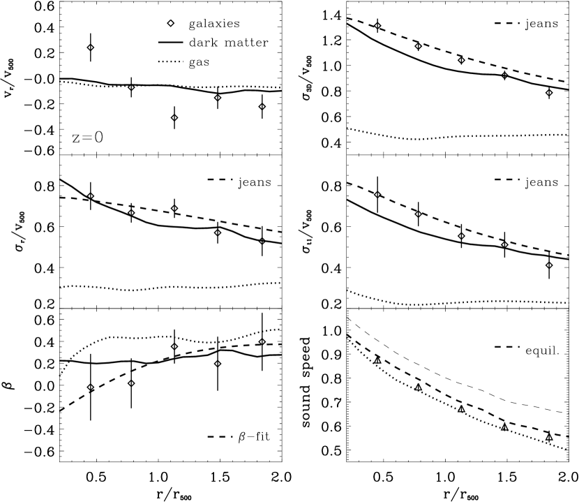
Figure 5: The radial profiles of kinematic properties of dark matter (solid), gas (dotted) and galaxies (diamonds), averaged over the sample of eight simulated clusters at $z=0$. Errorbars show 1 $\sigma$ errors of the mean. Upper-four panels: the mean radial velocity $v_{r}$ (top-left), the three dimensional velocity dispersion $\sigma_{\rm 3D}$ (top-right), and its radial and tangential components, $\sigma_{r}$ (middle-left) and $\sigma_{t}$ (middle-right). The dashed lines in these panels are the results derived using the Jeans equation. Bottom-left: the anisotropy parameter $\beta$. The dashed line is the best-fit $\beta$ profile of galaxies based on the formula (4). Bottom-right: the average sound speed of intracluster gas $c_{s}$. The triangles are the measurements of sound speed of gas ahead of galaxies, as sketched in Fig. 4. The dotted line is an average of the sound speeds in individual mesh cells. The two dashed lines show the solutions of the hydrostatic equilibrium equation, where we assumed $\sigma_{\rm turb}=0$ (thin dashed line) and $\sigma_{\rm turb}=\sigma_{\rm 3D}$[gas] (thick dashed line).

4.2 The equilibrium analysis

In this section, we apply the two equilibrium equations, the Jeans equation for galaxies and the hydrostatic equilibrium equation for intracluster gas to calculate velocity dispersion profiles under the assumptions that clusters are spherically symmetric and are in equilibrium. We then compare the results to the direct measurements of the velocity dispersion from the simulations to assess the validity of the equilibrium assumption.

4.2.1 The Jeans equation

We apply the Jeans equation to derive the average velocity dispersion of galaxies in galaxy clusters. For the relaxed systems with no rotational support ($\bar{v}_{r}=\bar{v}_{\theta}=0$), the Jeans equation is

$${1\over n_{\rm gal}}{\frac{d}{{d}r}}\left(n_{\rm gal}\sigma^{2}_{r}\right)+2\beta{\sigma^{2}_{r}\over r}=-{{d}\Phi\over{d}r}$$ (5)

where $\beta$ is the velocity anisotropy parameter in Eq. (3), $n_{\rm gal}$ denotes the number density of galaxies and $\Phi(r)={\rm G}M_{\rm tot}(r)/r$ is the gravitational potential of the cluster. Integration of the Jeans equation requires knowledge of (1) the total mass profile, $M_{\rm tot}$, (2) the number density profile of galaxies, $n_{\rm gal}$ and (3) the radial profile of the velocity anisotropy, $\beta(r)$. In order to solve the equation for the sample of clusters using the average profiles, it is convenient to work with the dimensionless variables. We, therefore, scale each variable using their values at $r_{500}$ and then construct an average profile for all eight clusters. For the number density of galaxies, we use the best-fit NFW profile discussed in § 3.2 (see also Fig. 2). For the velocity anisotropy profile, we use the fit to the actual measurements in simulations using the fitting formula of Colín et al. (2000, see eq. (4) above).

Using the derived values of $\sigma_{r}(r)$ and the best-fit $\beta(r)$ profile, we compute the tangential and total velocity dispersion profiles, $\sigma_{t}(r)$ and $\sigma_{\rm 3D}(r)$. These profiles are shown by the dashed lines in the corresponding panels of figure 5. All equilibrium solutions agree well with the values directly measured in simulations.

4.2.2 Hydrostatic equation

For a system in equilibrium, the hydrostatic equation

$${1\over\rho_{\rm gas}}{dp_{\rm gas}\over dr}=-{d\Phi\over dr}\$$ (6)

relates the gas density $\rho_{\rm gas}$ and gas pressure $p_{\rm gas}$, to the gravitational potential of the cluster, $\Phi(r)$. The gas sound speed is given by

$$c_{s}=\sqrt{\gamma\left({p_{gas}\over\rho}-{\sigma^{2}_{\rm turb}\over 3}\right)}\ .$$ (7)

Note that this expression takes into account the additional contribution to the pressure due to turbulent gas motions, where $\sigma_{\rm turb}$ denotes the three dimensional velocity dispersion of turbulent gas motions.

Using the hydrodynamical variables and the total mass profile $M_{\rm tot}(r)$ measured directly from the simulations, we solve for the sound speed of gas using the Eq. (6) and (7). To solve these equations, we perform similar scaling and interpolation discussed in the previous section on the measured quantities. The dashed lines in the bottom-right panel of the figure 5 show the results of the calculation. The thin and thick dashed lines show the sound speed calculated assuming $\sigma_{\rm turb}=0$ and $\sigma_{\rm turb}=\sigma_{\rm 3D}$[gas] respectively, where $\sigma_{\rm 3D}$[gas] is the velocity dispersion of the gas shown by the dotted line in the top-right panel. The figure shows that if random motions of gas are ignored, the sound speed is overestimated by $\approx 10\%$. This indicates that random motions contribute $\gtrsim 10\%$ to the total pressure support in simulated clusters, which is in agreement with recent observations (Schuecker et al., 2004). If we assume $\sigma_{\rm turb}=\sigma_{\rm 3D}$, the estimated sound speed of gas is in good agreement with the values measured directly from the gas density and thermal pressure.

4.3 The average Mach number of galaxy motions

To estimate the Mach number of galaxies, $M\equiv\bar{v}/c_{s}$ , we need to measure the average velocity of galaxy motions, $\bar{v}$, and the average sound speed of the intracluster gas, $c_{s}$. Below, we compute the Mach number of galaxies in two different ways. First, we measure the average Mach number of galaxies directly from the simulation by measuring the velocity of each galaxy and sound speed of gas immediately ahead of the galaxy in the direction of its motion, as sketched in figure 4. Once the Mach number is measured for all galaxies, we compute the average Mach number in the spherical bins and average over all clusters in the sample.

Alternatively, we can measure the average Mach number of galaxies using the results of the Jeans and hydrostatic equilibrium equations in the previous section. As we discussed in § 3.3 (see Fig. 3), the velocity distribution of galaxies is well-described by the Maxwell-Boltzmann distribution. This means that the mean velocity of galaxies can be calculated using their three dimensional velocity dispersion as

$$\bar{v}=0.92\sigma_{\rm 3D}.$$ (8)

We thus compute $\bar{v}$ from $\sigma_{\rm 3D}$ obtained by solving the Jeans equation. Similarly, we use the sound speed of gas, $c_{s}$, obtained from the hydrostatic equation. Note that estimating the sound speed of gas requires the knowledge of turbulent gas motions $\sigma_{\rm turb}$. Since characterising the nature of the turbulent gas motions is beyond the scope of the paper, we simply assume $\sigma_{\rm turb}=\sigma_{\rm 3D}$[gas], which has been shown to result in good agreement between the calculated and measured values of the sound speed in Fig. 5.

Figure 6 shows the average Mach number of galaxies in the simulated clusters. The diamonds are the direct measurement from the simulation, and the dashed line is calculated using solutions of the equilibrium equations. The figure shows that on average galaxies move supersonically with the average Mach number of $\sim 1.3-1.4$ throughout the cluster volume.

Figure 6: The Mach number of galaxies orbiting in the cluster environment. The diamonds show the direct measurements from the simulations, averaged over the sample of eight simulated clusters at $z=0$, and the error bars indicate the $1\sigma$ confidence interval. The dashed line is the result of the equilibrium equations, where we assumed that $\sigma_{\rm turb}=\sigma_{\rm 3D}$[gas] to account for the turbulent gas motions in the estimate of the sound speed of intracluster gas. The figure shows that galaxies move supersonically with the Mach number of $1.3-1.4$ throughout the cluster environment.

In the first approximation, the slightly supersonic motions of galaxies can be explained by the following simple argument. The mean velocity of galaxies is given by eq. (8), while the sound speed is $v_{s}=\left(\gamma P_{\rm gas}/\rho\right)^{1/2}$ $=\left(\gamma\sigma_{\rm gas}^{2}/3\right)^{1/2}$, where $\sigma_{\rm gas}^{2}$ is the velocity dispersion of the microscopic thermal motions of gas particles. If the three-dimensional velocity dispersions of gas particles and galaxies are approximately equal, as is expected in equilibrium, we have:

$$\langle M\rangle=\bar{v}/c_{s}\approx 0.92\sqrt{3/\gamma}\approx 1.23,$$ (9)

for $\gamma=5/3$. As was shown in the previous section, turbulent pressure contributes $>10\%$ to the total pressure and the sound speed is actually $\approx 10\%$ lower than what it would be without the turbulence. This can explain the average Mach number that we measure $\langle M\rangle\approx 1.23/0.9\approx 1.37$.

5 Discussion and Conclusions

We presented analysis of the galaxy motions in clusters using high-resolution cosmological simulations of the concordance flat $\Lambda$CDM model. The simulations follow dynamics of dark matter and gas and include various physical processes critical for galaxy formation: gas cooling, heating and star formation. These simulations, therefore, follow the formation of galaxies and their evolution in the dense cluster environment in a realistic cosmological context. Analysing motions of galaxies and the properties of intracluster gas in the sample of eight simulated clusters at $z=0$, we study velocity dispersion profiles of the dark matter, gas, and galaxies. We measure the mean velocity of galaxy motions and gas sound speed as a function of radius and calculate the average Mach number of galaxy motions.

Our simulations show that galaxies, on average, move supersonically throughout the cluster volume. The average Mach number is $\langle M\rangle\approx 1.4$, approximately independent of cluster-centric radius. The value of $\langle M\rangle$ can be attributed to the difference between the three-dimensional velocity of galaxies and one-dimensional sound speed and to the existence of the turbulent motions of gas (see eq. 9). The thermal pressure and, hence, the sound speed are smaller than would be required if all of the gas pressure support was due to thermal pressure. Also, gas and galaxies have somewhat different radial density and velocity anisotropy profiles. The motions of galaxies and gas particles are governed by the same potential, but non-zero velocity anisotropy and differences in the radial distribution can lead to different velocity dispersion and sound speed profiles.

We also find that galaxies move slightly faster than the dark matter particles in clusters, although the magnitude of the velocity bias, $b_{v}\approx 1.1$, is considerably smaller than the bias estimated for subhalos in dissipationless simulations (Colín et al., 2000; Ghigna et al., 2000; Diemand et al., 2004; Gao et al., 2004). Interestingly, we find velocity bias in the tangential component of the velocity dispersion, but not in the radial component. Despite the small sample size used in this analysis, we find that these results are robust and statistically significant. Namely, the results do not change if we analyse clusters by removing two of the least relaxed clusters at $z=0$ or using clusters at the epoch when they appear most relaxed. Nevertheless, it would be good to verify these results with higher resolution simulations and better statistics.

Our simulations show that the difference between the dark matter and galaxy velocity dispersions is significant only in the inner regions of clusters ($r/r_{500}\lesssim 0.7$). This is also where we find a corresponding difference in the velocity anisotropies. With these results in mind, we conjecture that the bias is likely caused by the preferential disruption of objects on highly radial orbits. In other words, galaxies on radial orbits are prone to more efficient tidal disruption than those on circular orbits with the same orbital energy, since galaxies on radial orbits pass closer to the dense central regions during their peri-centric passages. If the effect is significant, we expect the fraction of galaxies with the small (large) tangential (radial) velocity component to decrease in the inner regions of clusters. The distributions of $v_{r}$ ($v_{t}$), therefore, become progressively skewed towards smaller (larger) values with decreasing radius.

Our simulations show that this is indeed the case. Specifically, we find that the distributions of $v_{r}$ and $v_{t}$ become increasingly non-gaussian, and $v_{t}/v_{r}$ ratio increases monotonically at the smaller cluster-centric distances within $r<r_{500}$. Furthermore, if galaxies accrete onto clusters with the positive orbital velocity anisotropy, $\beta(r)>0$ (i.e., preference for the radial orbits), similar to dark matter particles, the tidal disruption would also drive the system toward more isotropic orbits. We indeed find that galaxy motions in the central regions of the clusters are nearly isotropic ($\beta\approx 0-0.1$), while the DM particles have the radial anisotropy of $\beta\approx 0.2-0.3$ (see Figure 5).

We also find considerable random bulk motions of gas. The 3D velocity dispersion is approximately constant as a function of radius: $\sigma_{\rm gas}\approx 0.4-0.5v_{500}$. In terms of the sound speed, the gas moves with the typical velocity of $\sigma_{\rm gas}/\sqrt{3}\sim 0.2-0.3c_{s}$ in the inner regions of clusters (see also Nagai et al., 2003; Sunyaev et al., 2003). Outside $r_{500}$, the typical velocities are $\sim 0.5c_{s}$, which reflects the increasing strength of the infall motions and lesser degree of relaxation. The random motions of gas contribute to the pressure support of galaxy clusters, in addition to the support from thermal pressure. We show that in our simulations, random motions contribute $\approx 10\%$ of the total pressure support. Recent X-ray observations of the Coma cluster also show evidence of random motions of gas of a similar magnitude (Schuecker et al., 2004). The non-thermal pressure support, if neglected, will bias measurement of the total mass in the hydrostatic analyses of the X-ray cluster observations by $\sim 10-20\%$.

The supersonic motions of cluster galaxies may be an important source of heating of the intracluster gas. Supersonically moving galaxies and groups can drive weak bow shocks and shock-heat the ICM (e.g. Markevitch et al., 2004; Finoguenov et al., 2004) or deposit energy via viscous dissipation of soundwaves (Ruszkowski et al., 2004). It is likely, however, that a more efficient heating mechanism is the transfer of the orbital energy of galaxy motions to the internal energy of gas via dynamical friction. Dynamical friction in the gaseous medium is efficient only if the perturber moves supersonically (Ruderman & Spiegel, 1971; Rephaeli & Salpeter, 1980; Just et al., 1990; Ostriker, 1999). Our results therefore confirm that this is a potentially viable heating mechanism. El-Zant et al. (2004) have recently argued that the dynamical friction heating is sufficiently efficient to prevent formation of the cooling flows in cluster cores. Their estimates show that in the Perseus cluster galaxies do move supersonically with the average Mach number of $M\sim 1.5-2$. For reasonable choices of the galaxy mass-to-light ratios the rate of energy loss to dynamical friction is sufficient to offset a cooling of gas in this cluster. El-Zant et al. (2004) also emphasise that this mechanism is self-regulating: as gas is heated, the galaxy motions become subsonic and heating becomes inefficient.

In principle, dynamical friction heating should be modelled self-consistently in cosmological simulations. Our simulations, however, do suffer from the well-known “overcooling problem:” the fraction of baryons in stars and cold gas is at least a factor of two higher than observed for the systems of the mass range we consider. For example, the typical star formation rate in the cool cores in the central galaxy in our clusters is $\gtrsim 1000\ {\rm M}_{\odot}{\rm yr}^{-1}$, which is much larger than is allowed by the observed values of the mass accretion rates (see e.g., Kaastra et al., 2004; Peterson et al., 2001, 2003; Tamura et al., 2001). This indicates that the dynamical friction heating is not efficient in our simulations. This could be due to their limited spatial resolution (a few kpc). It is possible, that to resolve the dynamical friction wakes properly a sub-kiloparsec resolution is needed. However, it is also possible that the wake formation is prevented by the random motions of the gas that we find in our simulations. These motions are much stronger than the gravitational pull of any individual galaxy and it is likely that galaxies simply cannot form wakes in such highly chaotic velocity field.

Given that dynamical friction can provide an attractive source of the ICM heating, it will be important to pursue this subject further. The progress can come both from the higher resolution cosmological simulations and from controlled gasdynamics experiments of a gravitating body moving in a gas flow. It would be interesting, for example, to test whether dynamical friction is equally efficient for a perturber moving in laminar and strongly turbulent flows.

References

- Berlind et al. (2003) Berlind A. A., Weinberg D. W., Benson A. J., Baugh C. M., Cole S., Davé R., Frenk C. S., Jenkins A., Katz N., Lacey C. G., 2003, ApJ, 593
- Binney & Tremaine (1987) Binney J., Tremaine S., 1987, Galactic dynamics. Princeton, NJ, Princeton University Press, 1987
- Blumenthal et al. (1986) Blumenthal G. R., Faber S. M., Flores R., Primack J. R., 1986, ApJ, 301, 27
- Churazov et al. (2002) Churazov E., Sunyaev R., Forman W., Böhringer H., 2002, MNRAS, 332, 729
- Colín et al. (2000) Colín P., Klypin A. A., Kravtsov A. V., 2000, ApJ, 539, 561
- Colín et al. (1999) Colín P., Klypin A. A., Kravtsov A. V., Khokhlov A. M., 1999, ApJ, 523, 32
- De Lucia et al. (2004) De Lucia G., Kauffmann G., Springel V., White S. D. M., Lanzoni B., Stoehr F., Tormen G., Yoshida N., 2004, MNRAS, 348, 333
- Desai et al. (2004) Desai V., Dalcanton J. J., Mayer L., Reed D., Quinn T., Governato F., 2004, MNRAS, 351, 265
- Diemand et al. (2004) Diemand J., Moore B., Stadel J., 2004, MNRAS submitted (astro-ph/0402160)
- Dressler & Gunn (1983) Dressler A., Gunn J. E., 1983, ApJ, 270, 7
- Einasto et al. (1984) Einasto J., Klypin A. A., Saar E., Shandarin S. F., 1984, MNRAS, 206, 529
- El-Zant et al. (2004) El-Zant A., Kim W., Kamionkowski M., 2004, MNRASsubmitted (astro-ph/0403696)
- Evrard et al. (1996) Evrard A. E., Metzler C. A., Navarro J. F., 1996, ApJ, 469, 494
- Fabian et al. (2002) Fabian A. C., Celotti A., Blundell K. M., Kassim N. E., Perley R. A., 2002, MNRAS, 331, 369
- Ferland et al. (1998) Ferland G. J., Korista K. T., Verner D. A., Ferguson J. W., Kingdon J. B., Verner E. M., 1998, PASP, 110, 761
- Finoguenov et al. (2004) Finoguenov A., Pietsch W., Aschenbach B., Miniati F., 2004, A&A, 415, 415
- Frenk et al. (1996) Frenk C. S., Evrard A. E., White S. D. M., Summers F. J., 1996, ApJ, 472, 460
- Gao et al. (2004) Gao L., De Lucia G., White S. D. M., Jenkins A., 2004, MNRASsubmitted (astro-ph/0405010)
- Gao et al. (2004) Gao L., White S. D. M., Jenkins A., Stoehr F., Springel V., 2004, MNRASsubmitted (astro-ph/0404589)
- Gavazzi et al. (1995) Gavazzi G., Contursi A., Carrasco L., Boselli A., Kennicutt R., Scodeggio M., Jaffe W., 1995, A&A, 304, 325
- Ghigna et al. (1998) Ghigna S., Moore B., Governato F., Lake G., Quinn T., Stadel J., 1998, MNRAS, 300, 146
- Ghigna et al. (2000) Ghigna S., Moore B., Governato F., Lake G., Quinn T., Stadel J., 2000, ApJ, 544, 616
- Gnedin (2003) Gnedin O. Y., 2003, ApJ, 589, 752
- Gnedin et al. (2004) Gnedin O. Y., Kravtsov A. V., Klypin A. A., Nagai D., 2004, ApJ, accepted (astro-ph/0406247)
- Gunn & Gott (1972) Gunn J. E., Gott J. R. I., 1972, ApJ, 176, 1
- Haardt & Madau (1996) Haardt F., Madau P., 1996, ApJ, 461, 20
- Hartmann (2002) Hartmann L., 2002, ApJ, 578, 914
- Hoeft et al. (2004) Hoeft M., Mücket J. P., Gottlöber S., 2004, ApJ, 602, 162
- Jungwiert et al. (2001) Jungwiert B., Combes F., Palouš J., 2001, A&A, 376, 85
- Just et al. (1990) Just A., Deiss B. M., Kegel W. H., Boehringer H., Morfill G. E., 1990, ApJ, 354, 400
- Kaastra et al. (2004) Kaastra J. S., Tamura T., Peterson J. R., Bleeker J. A. M., Ferrigno C., Kahn S. M., Paerels F. B. S., Piffaretti R., Branduardi-Raymont G., Böhringer H., 2004, A&A, 413, 415
- Kaiser (1991) Kaiser N., 1991, ApJ, 383, 104
- Katz et al. (1992) Katz N., Hernquist L., Weinberg D. H., 1992, ApJ, 399, L109
- Kennicutt (1998) Kennicutt R. C., 1998, ApJ, 498, 541
- Klypin et al. (1999) Klypin A., Gottlöber S., Kravtsov A. V., Khokhlov A. M., 1999, ApJ, 516, 530
- Klypin et al. (2001) Klypin A., Kravtsov A. V., Bullock J. S., Primack J. R., 2001, ApJ, 554, 903
- Koopmann & Kenney (2004) Koopmann R. A., Kenney J. D. P., 2004, ApJ, 613, 866
- Kravtsov (1999) Kravtsov A. V., 1999, PhD thesis, New Mexico State University
- Kravtsov et al. (2004) Kravtsov A. V., Berlind A. A., Wechsler R. H., Klypin A. A., Gottlöber S., Allgood B., Primack J. R., 2004, ApJ, 609, 35
- Kravtsov et al. (2002) Kravtsov A. V., Klypin A., Hoffman Y., 2002, ApJ, 571, 563
- Kravtsov et al. (1997) Kravtsov A. V., Klypin A. A., Khokhlov A. M., 1997, ApJS, 111, 73
- Markevitch et al. (2004) Markevitch M., Gonzalez A. H., Clowe D., Vikhlinin A., Forman W., Jones C., Murray S., Tucker W., 2004, ApJ, 606, 819
- Metzler & Evrard (1994) Metzler C. A., Evrard A. E., 1994, ApJ, 437, 564
- Miller & Scalo (1979) Miller G. E., Scalo J. M., 1979, ApJS, 41, 513
- Miller (1986) Miller L., 1986, MNRAS, 220, 713
- Miller & Owen (2003) Miller N. A., Owen F. N., 2003, AJ, 125, 2427
- Moore et al. (1999) Moore B., Ghigna S., Governato F., Lake G., Quinn T., Stadel J., Tozzi P., 1999, ApJ, 524, L19
- Moore et al. (1996) Moore B., Katz N., Lake G., Dressler A., Oemler A., 1996, Nature, 379, 613
- Nagai & Kravtsov (2005) Nagai D., Kravtsov A. V., 2005, ApJ, in press (astro-ph/0408273)
- Nagai et al. (2003) Nagai D., Kravtsov A. V., Kosowsky A., 2003, ApJ, 587, 524
- Navarro et al. (1996) Navarro J. F., Frenk C. S., White S. D. M., 1996, ApJ, 462, 563
- Navarro et al. (1997) Navarro J. F., Frenk C. S., White S. D. M., 1997, ApJ, 490, 493
- Nulsen (1982) Nulsen P. E. J., 1982, MNRAS, 198, 1007
- Okamoto & Habe (1999) Okamoto T., Habe A., 1999, ApJ, 516, 591
- Ostriker (1999) Ostriker E. C., 1999, ApJ, 513, 252
- Pearce et al. (1999) Pearce F. R., Jenkins A., Frenk C. S., Colberg J. M., White S. D. M., Thomas P. A., Couchman H. M. P., Peacock J. A., Efstathiou G., The Virgo Consortium 1999, ApJ, 521, L99
- Peterson et al. (2003) Peterson J. R., Kahn S. M., Paerels F. B. S., Kaastra J. S., Tamura T., Bleeker J. A. M., Ferrigno C., Jernigan J. G., 2003, ApJ, 590, 207
- Peterson et al. (2001) Peterson J. R., Paerels F. B. S., Kaastra J. S., Arnaud M., Reiprich T. H., Fabian A. C., Mushotzky R. F., Jernigan J. G., Sakelliou I., 2001, A&A, 365, L104
- Quilis et al. (2000) Quilis V., Moore B., Bower R., 2000, Science, 288, 1617
- Reed et al. (2004) Reed D., Governato F., Quinn T., Gardner J., Stadel J., Lake G., 2004, MNRASsubmitted (astro-ph/0406034)
- Rephaeli & Salpeter (1980) Rephaeli Y., Salpeter E. E., 1980, ApJ, 240, 20
- Rose et al. (2001) Rose J. A., Gaba A. E., Caldwell N., Chaboyer B., 2001, AJ, 121, 793
- Ruderman & Spiegel (1971) Ruderman M. A., Spiegel E. A., 1971, ApJ, 165, 1
- Ruszkowski et al. (2004) Ruszkowski M., Brüggen M., Begelman M. C., 2004, ApJ, 611, 158
- Sakai et al. (2002) Sakai S., Kennicutt R. C., van der Hulst J. M., Moss C., 2002, ApJ, 578, 842
- Scannapieco & Oh (2004) Scannapieco E., Oh S. P., 2004, ApJ, 608, 62
- Schuecker et al. (2004) Schuecker P., Finoguenov A., Miniati F., Boehringer H., Briel U. G., 2004, A&Asubmitted (astro-ph/0404132)
- Schulz & Struck (2001) Schulz S., Struck C., 2001, MNRAS, 328, 185
- Sunyaev et al. (2003) Sunyaev R. A., Norman M. L., Bryan G. L., 2003, Astronomy Letters, 29, 783
- Tamura et al. (2001) Tamura T., Kaastra J. S., Peterson J. R., Paerels F. B. S., Mittaz J. P. D., Trudolyubov S. P., Stewart G., Fabian A. C., Mushotzky R. F., Lumb D. H., Ikebe Y., 2001, A&A, 365, L87
- Tormen et al. (1998) Tormen G., Diaferio A., Syer D., 1998, MNRAS, 299, 728
- Valageas & Silk (1999) Valageas P., Silk J., 1999, A&A, 350, 725
- Voit & Ponman (2003) Voit G. M., Ponman T. J., 2003, ApJ, 594, L75
- Vollmer (2003) Vollmer B., 2003, A&A, 398, 525
- Vollmer et al. (2001) Vollmer B., Cayatte V., Balkowski C., Duschl W. J., 2001, ApJ, 561, 708
- Weinberg et al. (2004) Weinberg D. H., Davé R., Katz N., Hernquist L., 2004, ApJ, 601, 1
- Woosley & Weaver (1995) Woosley S. E., Weaver T. A., 1995, ApJS, 101, 181
- Yoshikawa et al. (2001) Yoshikawa K., Taruya A., Jing Y. P., Suto Y., 2001, ApJ, 558, 520
- Zheng et al. (2004) Zheng Z., Berlind A. A., Weinberg D. H., Benson A. J., Baugh C. M., Cole S., Davé R., Frenk C. S., Jenkins A., Katz N., Lacey C. G., 2004, ApJsubmitted