The Cosmic Ray Muon Flux at WIPP

Abstract

In this work a measurement of the muon intensity at the Waste Isolation Pilot Plant (WIPP) near Carlsbad, NM, USA is presented. WIPP is a salt mine with a depth of 655 m. The vertical muon flux was measured with a two panels scintillator coincidence setup to $\Phi_{vert}~{}=~{}(3.10^{+0.05}_{-0.07})~{}10^{-7}$ s^-1cm^-2sr^-1.

1 Introduction

The cosmic ray background consists of several different particles such as pions, electrons, protons, etc. They are coming either from space or are generated in the high atmosphere. The most numerous generated underground are muons that are created when protons and secondary particles interact with atoms in the atmosphere. Experiments can be shielded from this cosmic activity by going deep underground. In this paper we describe a measurement of the cosmic ray muon flux at the Waste Isolation Pilot Plant (WIPP) with an overburden of 655 m of rock and salt and located 30 miles east of Carlsbad, New Mexico DOE (01). Such measurements are useful in assessing the appropriateness of WIPP as a site for underground experiments that require shielding from cosmic radiation. The depth requirements and adequacy of a particular site vary depending on the nature and goals of a particular experiment. This paper does not attempt to address the appropriateness of the WIPP site as a general purpose underground laboratory, an exercise of intense activity within the scientific community at present. Such a task is beyond the scope of this paper. The paper focuses on the measurements of the muon flux at WIPP, which serves as an important input in evaluating the impact on specific experiments.

2 Experimental Setup

The experiment to measure the muon flux in the underground of WIPP was conducted 655 meters below the surface in the experimental Q-Area. The detector consisted of two plastic scintillator panels each 305 cm long, 76.2 cm wide and 2.54 cm thick. Each panel had two light-guides mounted on the two narrow ends. A 12.7 cm diameter photo-tube with an operating voltage of 800 volts was mounted on each light-guide enabling a double ended readout. The muon detection efficiency as a function of position for each panel was measured by placing two small scintillators above and below. If the small detectors triggered coincident, a muon must have passed through the large panel. The number of events in the panel over the total number of triggers gives therefore the muon detection efficiency. Each position was tested with 10,000 coincidence events. High energy, minimum ionizing muons would deposit about 5 MeV when traversing a scintillator paddle at normal incidence. The actual energy spectrum deposited in the Patel exhibits a broad tail around this pronounced peak due to muons traversing at angles other than normal, straggling effects, and the finite energy resolution of the scintillator. Nonetheless, by summing the signal heights from the PMT’s of each panel with a threshold of 3 MeV, a clean muon signal can be obtained well above the electronic noise and low energy gamma background associated with a single PMT channel. The detector efficiency for muons was found to be 100$\pm 1$% for all positions.

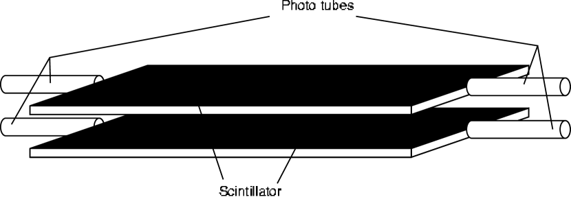
Figure 1: Setup of the scintillator panels. They were placed on top of each other with a distance of 30.5 cm.

For the actual experiment panel 1 was mounted on top of panel 2 in a distance of 30.5 cm (see Fig. 1). A fourfold coincidence from the photo-tubes was required to record an event. The high voltage on each photo-multiplier tube (PMT) was adjusted by demanding an equal pulse height for a ⁹⁰Sr calibration source place in the center of each panel. The decay product of ⁹⁰Sr is ⁹⁰Y which decays emitting high energy electrons, which were detected in the panel. Fig. 2 shows the electronic diagram. The pre-amplifier signal had a rise time of 10 ns to 20 ns. It was split up and one signal was fed through a spectroscopic amplifier with a shaping time of 0.25 $\mu$s and connected to an LeCroy AD811 ADC. The other signal was put into a discriminator with a 175 mV threshold which was equivalent to an energy of 1.1 MeV. The steep NIM pulses from the discriminators were used as input for a coincidence unit. Fig. 3 illustrates the timing for the different components during an event. The coincidence window had a width of 100 ns. The output of the coincidence was then processed by a gate/delay generator and used as strobe for the ADC. The strobe window was chosen to be 0.5 $\mu$s wide. This ensured that the peak from the spectroscopic amplifier was inside the ADC strobe window.

3 Data Analysis

The experiment was conducted during a run-time of 6.17 days. Panel one had a slightly better resolution than panel two. This was due to an increased noise in photo tube 3. The total charge in a panel was calculated as the sum of the outputs of its two PMTs.

To determine the energy calibration of the detectors Monte-Carlo simulations were carried out with Geant 4. The initial energy distribution of the muons simulated was derived from the following empirical formula corrected for the energy losses in 655 m of rock and salt MIY (73):

$$N(P)dP = AP^{-\alpha}\,dP\mbox{ with}$$ (1)

$$\alpha = 0.5483+0.3977\ln P\mbox{ and}$$

$$A = 3.09\times 10^{-3}\mbox{cm}^{-2}\mbox{s}^{-1}\mbox{sr}^{-1}(\mbox{GeV}/c)^{-1},$$

$P$ being in GeV/c. The intensity distribution of the polar angle $\theta$ was taken from MIY (73). A simplified angular distribution for medium depth can be written as MIY (73)

$$\Phi(h,\theta) = \Phi(h,0)\cos^{1.53}\theta e^{-8.0\times 10^{-4}h(\sec\theta-1)}.$$ (2)

with $\Phi(h,\theta)$ as the flux for a specific angle in cm^-2s^-1sr^-1. Figure 4 shows this spectrum at sea level. The energy calibration was done by fitting the maximum intensity of the muon peak to the maximum intensity of the Monte-Carlo for the detector. A comparison of measured and simulated data is shown in Fig. 5 for both panels.

The total muon spectrum for each panel was achieved by adding the ADC values of both photo tubes up on an event-by-event base. The different energy resolutions of the PMT’s were taken into account during the Geant 4 simulations (see difference between upper and lower panel in Fig. 5). For more details see ESC (01). The shape of the measured spectrum could be reproduced within statistical uncertainties. The muon peak with its maximum intensity around 4.8 MeV is clearly visible.

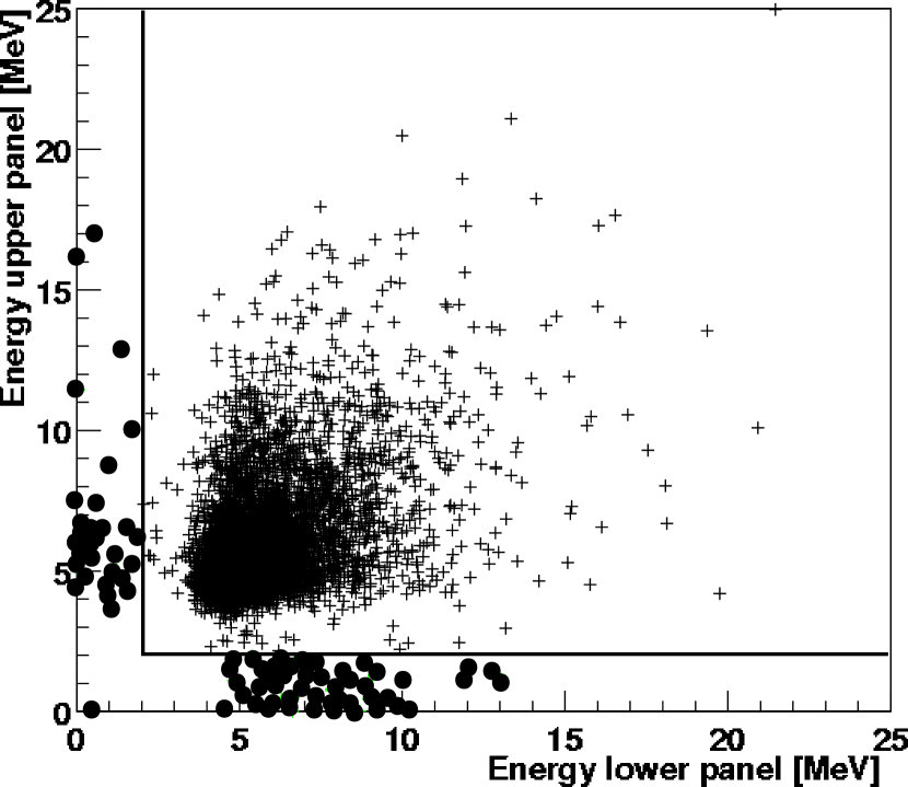
Figure 7: Two dimensional spectrum for the cuts applied to the muon Monte-Carlo simulation. The spectrum shows on the x-axis the deposited energy in MeV for the lower panel, on the y-axis the deposited energy for the upper panel. The black line displays the cut chosen for the muon number. The events marked by a cross represent the muon peak, the events marked by a dot represent muons outside the cut region. The ratio of these muons in the simulation is $1.24\pm 0.01\%$.

Fig. 6 shows a two dimensional plot of an event by event energy distribution for the two panels. The x-axis shows the energy deposition in the lower panel the y-axis the energy deposition in the upper panel. Among the events marked with a cross, the muon peak is clearly visible at approximately 5 MeV energy deposition in each panel. A cut above 2 MeV energy deposition for each panel was chosen to determine the number of muons. The black line represents the cutting border. Fig. 7 shows the same cut applied to the Monte-Carlo simulations. According to the Monte-Carlo simulations $1.24\pm 0.01\%$ of the muon events are cut out. The low energy events in Fig 6 are due to PMT noise, which are therefore absent in Fig. 7. Table 1 contains the integral information of the different regions in the spectrum shown in Fig 6. The errors quoted are purely statistical errors. The final muon peak cut is shown by cut 6 and the muon number derived from the cut is

$$N_{\mu} = 5202\pm 72,$$ (3)

where the uncertainty is statistical only.

The next step is to determine how many counts of the background contributed into the signal and how many counts from the signal were lost into the low energy background due to the cut. The trigger rate coming from two photo tubes in one panel in coincidence was 220$\pm$10 Hz. As described above, during the experiment the data were taken demanding a quadruple coincidence, which basically means a coincidence between the two panels. The random coincidence rate can therefore be calculated with

$$\nu_{r} = 2\nu_{1}\nu_{2}\tau,$$ (4)

where $\nu_{r}$ is the random coincidence frequency, $\nu_{1}$ and $\nu_{2}$ the two frequencies and $\tau$ the coincidence window. With a coincidence window of $100\pm 5$ ns the rate can be calculated to$\nu_{r}=9.68\pm 0.79\times 10^{-3}\mbox{ Hz}$ or 5158 $\pm 43$ counts. The main part of the background can be attributed to random coincidences (see first cut 0 of Table 1) the tail of the background was assumed to be exponential and extrapolated into the region of interest. The results are listed in Table 2. The number of muon induced events outside the region of interest was estimated using the result of the Monte-Carlo simulations (see Fig. 7 and Table 1).

The muon flux can be calculated as follows.

$$\Phi_{total} = \frac{N_{0}}{\epsilon\cdot a\cdot t_{rt}},$$ (5)

where $\Phi_{total}$ is the total flux of muons through the panel, $N_{0}$ the measured number of muons, $\epsilon$ the efficiency of the detector which includes both the physical efficiency of the scintillator and the geometrical efficiency due to the setup of the detector and the angular distribution of the muons, $a$ the area covered by the detector (2.33 m²) and $t_{rt}$ the run-time of the experiment which was 532800 seconds.

The deviation of the geometrical efficiency from 100% results from the fact that not all muons pass the upper plate vertically. By requiring a coincidence between the upper and the lower panel, the measured number of muons will therefore be less than the number of muons passing through the upper panel. The deviation of the geometrical efficiency was determined by simulating two surfaces with size of the scintillator panels with a separation of 30.5 cm. The start positions for the muons were randomly chosen on the upper panel. The azimuthal direction was sampled randomly in an interval between 0 and 2$\pi$. The simulations were carried out with a lateral distribution according to equation 2. The depth parameter h was varied over a range of $\pm$10%. With a measured density of (2.3$\pm$0.2) g/cm³ LAB (95) an efficiency of (88.5$\pm 0.2$)% was obtained. The vertical flux can be calculated using the approximating formula from MIY (73)

$$\Phi(h,\theta) = \Phi(h,0)\cos^{1.53}\theta,$$ (6)

for a depth of 1526 m.w.e. the vertical flux is $\Phi_{vert}=\left(0.65\pm 0.04\right)\times\Phi_{tot}$.

3.1 Backgrounds

In the following section other sources of background than discussed in previous sections are estimated. In order to generate a coincidence pulse with an energy deposition of more than the threshold of 2.0 MeV one has to look at particles with higher energy.

3.1.1 Neutrons from Muons

Neutrons generated from muons traversing through the rock and salt are one candidate for the expected background in the WIPP. In his paper Bezrukov BEZ (73) estimates the amount of neutrons per muon generated at a depth of 1500 meter water equivalent (m.w.e.) in hg/cm² to

$$N_{n(\mu)} = 7~{}10^{-4}\frac{\mbox{cm}^{2}}{\mbox{g}}.$$ (7)

With equation the empirical equation from MIY (73)

$$\Phi(h,0) = \frac{174}{h+400}\left(h+10\right)^{-1.53}\mbox{e}^{-8.0\times 10^{-4}h},$$ (8)

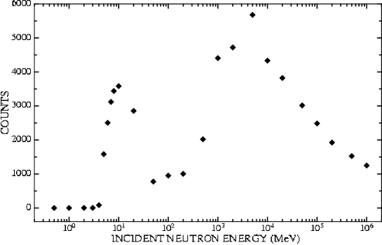
Figure 8: Neutron efficiency of the two panels as a function of primary neutron energy.

where $\Phi$ has the units of (cm s sr )^-1 and h represents the depth in $hg/cm^{2}$, this calculates to a neutron flux of $3.36$ $10^{-7}~{}\mbox{kg}^{-1}\mbox{s}^{-1}$. With an assumed average cross section of 1 barn the attenuation length in salt is 21 cm. This calculates to a neutron flux of $1.6$ $10^{-8}~{}{\mbox{cm}^{-2}\mbox{s}^{-1}}$, or $8.6$ $10^{-3}~{}\mbox{cm}^{-2}$ during the entire length of experiment of 6.17 days. Several Monte-Carlo simulations have been carried out to estimate the detection efficiency for neutrons in the existing detector geometry. The neutrons were randomly started from a sphere of 2 m radius surrounding the two panels into the whole solid angle. Several simulations with neutron energies ranging from 500 keV to 1 TeV were performed (see Fig. 8). According to the experimental settings, only such events were counted, where both panels had an energy deposition between 2 and 20 MeV. The most important interaction mechanism is inelastic scattering on hydrogen and carbon in the scintillator material. Therefore the number of events depositing at least 2 MeV in each of the panels is reduced by at least 3 orders of magnitude, if the incident neutron energy falls below 4 MeV. Only neutron captures and other nuclear channels can than produce the required energy. The number of simulated events in Fig. 8 corresponds to 20 neutrons/cm². Scaling this number to the expected number of neutrons during the experiment and assuming the highest efficiency, gives an upper limit for the number of neutron induced events of $N_{neutron}~{}=~{}2.6$. Most of the neutrons will be moderated by the time they reach the detector. The assumption made above is, therefore, very conservative.

3.1.2 Neutrons from U and Th

Natural radioactivity is present in every geological layer of the earth. An abundance of uranium and thorium in the salt is able to generate neutrons via ($\alpha,n$)-reactions and through spontaneous fission. The U and Th contents at WIPP have been measured WEB (98) and are displayed in Table 3. With the numbers from FLO (88) for neutron production via ($\alpha,n)$-reactions of U and Th in salt, who lists U_(α,n)=5.07 10^-8 s^-1g^-1 for an uranium abundance of 0.3 ppm and Th_(α,n)=1.51 10^-7 s^-1g^-1 for a thorium abundance of 2.06 ppm in salt, one can estimate the neutron production rate to U_(α,n)=8.11 10^-9 s^-1g^-1 for an uranium abundance of 0.048 ppm and Th_(α,n)=1.83 10^-8 s^-1g^-1 for a thorium abundance of 0.25 ppm in salt (according to column ”Used Values” in Table 3). Assuming again an attenuation length of 21 cm leads to an upper neutron flux of 1.28 10^-6 s^-1g^-1. Since the highest alpha generated in the U/Th decay chain has ca. 8 MeV and the Q-values of the (n,$\alpha$) reactions at Na or Cl is at most -3 MeV, a maximum neutron energy of 5 MeV can be assumed. With the simulation results from Fig. 8 this leads to a neutron number in the panels of $N_{U,Th}=54$ during the measurement.

3.1.3 Gamma Background

There are two main sources of gamma background, first the decay of U/Th, and second the decay of ⁴⁰K. The highest level of gamma background comes from the decay of ⁴⁰K, which is abundant in the surrounding salt. The abundance of potassium in salt is 784 $\mu$g/g (see Table 3) and corresponds to $1.5~{}10^{15}$ ⁴⁰K/g. A 1.46 MeV $\gamma$-ray will be emitted during the decay, with a probability of 10.7%. With an half-life of $t_{1/2}=1.28~{}10^{9}$ y this results in a decay rate of approximately 2.7 10^-3 s^-1g^-1. With the macroscopic scattering cross section from BER (01) of $\sigma$=$5.02~{}10^{-2}$ b in NaCl and the assumption of an exponential attenuation law, an attenuation length of 8.4 cm is computed. The attenuation length is defined as the length after which the intensity drops by a factor e. With a salt density of 2.3 g/cm³ the amount of salt contributing $\gamma$-rays can then be estimated to 19.3 g/cm², which results in a $\gamma$-flux of $\Phi_{\gamma}$ = 5.22 10^-2 s^-1cm^-2. Since each gamma can deposit at most 1.46 MeV, a triple coincidence during the coincidence window of 100 ns in the detector is required to generate a signal inside the muon-cut region. According to the GEANT simulations, a $\gamma$-ray between 1 and 2 MeV emitted from a sphere of 2 m radius around the panels deposits energy with a probability less than 1% in one of the detectors, resulting in a rate of 262 s^-1 energy-depositing events. The resulting rate of triple coincidences ($\tau^{2}\nu^{3}$ with $\tau$ = 100 ns and $\nu$ = 262 s^-1) is 1.80 10^-7 s^-1, or 0.1 events during the experiment, hence negligible.

The number of gammas originating from $(n,\alpha)$ and $(n,\gamma)$ reactions can be estimated using the above calculated neutron flux. Assuming that only one $\gamma$-ray above 5 MeV is produced per neutron, the flux is 1.28 10^-6 s^-1g^-1. Gamma rays with energies up to 10 MeV have been simulated in order to estimate the efficiency of the muon panels including the coincidence requirement of at least 2 MeV energy deposition per panel. The geometry and number of particles were the same as described above for the neutrons (see Table 4). Assuming that the detection efficiency was on average below the simulated efficiency for a 10 MeV $\gamma$-ray, at most of 32 counts are expected during the entire run of the experiment.

3.2 The Muon-Flux

The raw data have (5202$\pm$72) counts in the region of interest. After the correction for electronic noise inside the region of interest (40$\pm$4) events and muon-induced events outside this region (62$\pm$6) events one obtains (5224$\pm 72\pm 7$) counts. A conservative 10% uncertainty was assumed for each of the corrections, which were then quadratically combined (see Table 5). Only upper limits for the contribution from neutrons (55) and $\gamma$-rays (32) have been performed. The uncertainty due to the detection efficiency is ($\pm$55) events. Since all the uncertainties are independent from each other, a quadratical addition of the different components can be performed. The final number of muon induced events in the muon panels is therefore ($5224^{+89}_{-108}$). As discussed above, the geometrical efficiency, resulting from the fact that not all muons are vertically, has to be taken into account. The number of muons passing through the detector area is ($5902^{+102}_{-123}$) events. The uncertainties of both, the surface area of the detector and the running time is well below the 1% level and can therefore be neglected.

Now the muon flux can be calculated:

$$\Phi_{tot} = \frac{5902^{+102}_{-123}}{532800\,s\times 23225\,\mbox{cm}^{2}}$$ (9)

$$= (4.77^{+0.08}_{-0.10})\times 10^{-7}\,\,\frac{\mbox{Hz}}{\mbox{cm}^{2}}$$

This flux can now be converted to a vertical flux of

$$\Phi_{vert} = (3.10^{+0.05}_{-0.07})\times 10^{-7}\,\,\frac{\mbox{Hz}}{\mbox{cm}^{2}\,\mbox{sr}},$$ (10)

converting to a meter water equivalence of ($1585^{+11}_{-6}$) m. Measurements made in the past in different underground laboratories in the world CRO (87), AMB (95) and AND (87) show similar results for this depth. The shallow depth agrees within its error bar with a fit through the previous experiments. Fig. 9 shows WIPP in comparison to other underground laboratories. With its average density of (2.3$\pm$0.2) g/cm³ and a depth of 655 m our measurement fits very well with the predicted data.

4 Conclusion

The work described here has determined the vertical muon flux at the WIPP mine to $\Phi_{vert}~{}=~{}(3.10^{+0.05}_{-0.07})$ $10^{-7}$ s^-1cm^-2sr^-1. This result agrees well with measurements at other underground laboratories and can now serve as an experimental basis for low-background experiments.

5 Acknowledgments

We would like to thank the WIPP staff, especially Roger Nelson, Dennis Hoffer and Dale Parish for their excellent support and generous help. We also want to acknowledge the help of M. Anaya and W. Teasdale for their technical support. This work was partially funded by LDRD funds from LANL and DOE.

Table 1: Cuts applied to determine event numbers in muon peak.

Cut	Cut	Cut	Events	Count rate
Number	Upper	Lower		[$Hz$]
	Panel	Panel
0	E$<$2 MeV	E$<$2 MeV	5207$\pm$ 72	9.8$\pm$0.14 $\times 10^{-3}$
1	—	—	11226$\pm$ 106	2.11$\pm$0.02 $\times 10^{-2}$
2	E$<$2 MeV	—	5881$\pm$77	1.10$\pm$0.014 $\times 10^{-2}$
3	—	E$<$2 MeV	5350$\pm$73	1.00$\pm$0.014 $\times 10^{-2}$
4	E$>$2 MeV	—	5345$\pm$73	9.7$\pm$0.14 $\times 10^{-3}$
5	—	E$>$2 MeV	5876$\pm$77	9.8$\pm$0.14 $\times 10^{-3}$
6	E$>$2 MeV	E$>$2 MeV	5202$\pm$72	9.9$\pm$0.14 $\times 10^{-3}$

Table 2: Tail fits of the background and muon signal.

Tail Name	Fit Interval		counts
Monte-Carlo cut off	0–	2.0 MeV	62
background upper panel	1.2–	2.1 MeV	20
background lower panel	1.0–	2.4 MeV	40

Table 3: Natural radioactivity at the WIPP-underground. The abundance of the elements was measured with mass spectrometry and gamma spectrometry by WEB (98). The Averages for the measurements are shown in the first two columns. The column labeled Used Value displays the value recommended by WEB (98). The values for the columns in soil were typical measurement of regular ground dirt gathered in southern New Mexico. The las column displays the ratio of the typical soil value over the corresponding WIPP number.

	at WIPP			Range in Soil			Ratio
	Mass	Gamma	Used	low	high	typical	Soil
	Spec.	Spec.	Value				vs.
Element	$\left[\frac{\mu g}{g}\right]$	$\left[\frac{\mu g}{g}\right]$	$\left[\frac{\mu g}{g}\right]$	$\left[\frac{\mu g}{g}\right]$	$\left[\frac{\mu g}{g}\right]$	$\left[\frac{\mu g}{g}\right]$	WIPP
Uranium	0.048	$<$0.37	0.048	0.5	2.5	1.5	30
Thorium	0.08	0.25	0.25	1.2	3.7	2.4	10
Potassium	784	182	480	500	900	700	1.5

Table 4: Number of events fulfilling the requirement of at least 2 MeV energy deposition per panel. 10⁷ gammas and neutrons were started from a sphere of 2 m radius around the muon panels.

Energy	Events
0.5 MeV	0
1 MeV	0
2 MeV	0
3 MeV	0
4 MeV	1
5 MeV	306
6 MeV	621
7 MeV	814
8 MeV	916
10 MeV	947

Table 5: The contributing parameter for the muon flux.

Name of parameter	Contribution
Runtime of the experiment	532800 seconds
Events in muon peak	5224$\pm$72 Events
Contribution background to signal	-40$\pm$4 Events
Muon induced events below threshold	+62$\pm$6 Events
Neutrons from U and Th	-54 Events
Neutrons from muons in rock	-2 Events
Gamma rays	-32 Events
Detector Efficiency	100 $\pm$ 1%
Detector Efficiency (geometric)	84.25% $\pm$ 0.4%
Conversion factor to vertical flux	0.65 $\pm$ 0.04

Figure 2: Setup of the scintillator-electronics. The electronics was setup in a quad coincidence mode. The signal coming from the photo-multiplier-tube (PMT) was amplified by a Phillips Scientific fast amplifier (777) with a gain of 20. This output signal was split. One signal was used as input for a discriminator attached to a coincidence unit to form the strobe for the LeCroy AD811 ADC. The other output was run through a shaping amplifier (S. A.) into the input channels of the ADC.

Figure 3: Timing of the scintillator Coincidence.

Figure 4: Differential muon intensity versus muon momentum.The spectrum is an empirical fit of the momentum distribution of vertical muons at sea level. The spectrum has a flat maximum at about 0.5 GeV/c.

Figure 5: Spectrum for the raw energy in the two scintillator panels. The energy is plotted into a histogram in units of  MeV, the Monte-Carlo simulation is shown as dotted line.

Figure 6: Two dimensional spectrum for the cuts applied to the muons. The spectrum shows on the x-axis the deposited energy in MeV for the lower panel, on the y-axis the deposited energy for the upper panel. The black line displays the cut chosen for the muon number. The events marked by a cross represent the muon peak, the events marked by a dot are dominated by the random coincidence of the PMTs.

Figure 9: Vertical muon flux for different underground experiments. The errors are smaller than the data marker.

References

- AMB (95) M. Ambrosio et al., (MACRO Colaboration), Phys. Ref. D Vol.52 3793 (1995).
- AND (87) Y.M. Andreev, V.I. Gurenzov and I.M. Koagi, Proc. 20th Int. Cosmic Ray Conf. (Moscow) Vol.6 200 (1987).
- BER (01) M.J. Berger, J.H. Hubbell, and S.M. Seltzer, http://physics.nist.gov/PhysRefData/Xcom/Text/XCOM.html.
- BEZ (73) Bezrukov, L.B., Beresnev, V.I., Zatsepin, G.T., Ryazhskaya, O.G., Stepanets, L.N., Yadernaya Fizika, Vol. 17, No.1, 98 (1973).
- CRO (87) M. Crouch, Proc. 20th Int. Cosmic Ray Conf. (Moscow) Vol.6 165 (1987).
- DOE (01) Department of Energy Carlsbad Field Office, Environmental Assesment, DOE/EA-1340 http://www.wipp.ws/library/ea/ea.htm (2001).
-
ESC (01)
E.-I. Esch, Thesis,
http://bibd.uni-giessen.de/gdoc/2001/uni/d010105.pdf (2001). - FLO (88) T. Forkowski, L. Morawska and K. Rozanski, Nucl. Geophys., 2, 1 (1988).
- LAB (95) M.A. Labreche, M.A. Beikmann, J.D. Osnes, B.M. Butcher, Sandia-Report SAND94-0890 UC-721.
- MIY (73) S. Miyake, 13th int. cosmic ray conf. Denver, CO Vol. 5 3638 (1973).
- WEB (98) J. Web, personal conversation at Carlsbad Environmental Monitoring and Research Center (1998).