The star formation history of Seyfert 2 nuclei

Abstract

We present a study of the stellar populations in the central $\sim 200$ pc of a large and homogeneous sample comprising 79 nearby galaxies, most of which are type 2 Seyferts. The star-formation history of these nuclei is reconstructed by means of state-of-the art population synthesis modeling of their spectra in the 3500–5200 Å interval. A QSO-like featureless continuum (FC) is added to the models to account for possible scattered light from a hidden AGN.

We find that: (1) The star-formation history of Seyfert 2 nuclei is remarkably heterogeneous: young starbursts, intermediate age, and old stellar populations all appear in significant and widely varying proportions. (2) A significant fraction of the nuclei show a strong FC component, but this FC is not always an indication of a hidden AGN: it can also betray the presence of a young, dusty starburst. (3) We detect weak broad H$\beta$ emission in several Seyfert 2s after cleaning the observed spectrum by subtracting the synthesis model. These are most likely the weak scattered lines from the hidden Broad Line Region envisaged in the unified model, given that in most of these cases independent spectropolarimetry data finds a hidden Seyfert 1. (4) The FC strengths obtained by the spectral decomposition are substantially larger for the Seyfert 2s which present evidence of broad lines, implying that the scattered non-stellar continuum is also detected. (5) There is no correlation between the star-formation in the nucleus and either the central or overall morphology of the parent galaxies.

1 Introduction

Our understanding of how galaxies form and evolve has changed in a rather unexpected way in recent years. On the one hand, massive black-holes now appear to populate the nuclei of virtually every (massive enough) galaxy. On the other, the nuclei of active galaxies (AGN), previously thought to be the only galaxies that harbored massive black-holes, are now known to be the hosts of massive star-forming regions. Hence, black-holes and starburst clusters coexist and are ubiquitous in the nuclear regions of galaxies.

The observational evidence for this scenario is abundant. The presence of strong CaII triplet absorptions in a large sample of Seyfert 2s and some Seyfert 1s provided the first direct evidence for a population of red super-giant stars in their nuclear regions (Terlevich, Díaz & Terlevich 1990). The absence of signs of a Broad Line Region (BLR) in the direct optical spectra of Seyfert 2 nuclei which show broad lines in polarized light can only be understood if there is an additional central source of blue/UV continuum associated with the obscuring torus (Cid Fernandes & Terlevich 1995). This conclusion is further supported by observations that polarization is lower in the continuum than in the scattered broad lines (Miller & Goodrich, 1990; Tran 1995a,b)

Most of the UV to near-IR continuum light in a number of Seyfert 2s, in particular all those so far observed with HST, is due to nuclear starbursts that are resolved in HST images. In some of these galaxies, the starburst luminosities are comparable to those of their ionizing engines. Thus, an observer situated along the axis of the torus will detect comparable contributions to the optical continuum coming from the starburst and from the broad line region components (Heckman et al. 1995, 1997). Massive star forming regions are even found in the nuclei of powerful radio galaxies through the detection of Balmer absorption lines or strong CaII triplet lines (Melnick et al. 1997; Aretxaga et al. 2001; Wills et al. 2002), showing that the intimate link between nuclear activity and star-formation exists not only in spiral galaxies, but also in massive ellipticals.

We have been engaged in a large spectroscopic survey of the nearest Seyfert galaxies in the southern hemisphere aimed at characterizing the properties of nuclear star-forming regions as a first step to understand the link between nuclear starbursts and massive black holes. The first results of this project were reported in Joguet et al. (2001, hereafter J01), where high S/N observations of about 80 Seyfert 2 galaxies were presented. This first inspection of the data revealed that about 50% of Seyfert 2s exihibit clear spectral signatures of star-formation in the recent past ($\la 100$ Myr), most notably high-order Balmer lines in absorption. The other half of the sample is equally split between nuclei with strong emission lines but weak absorption lines and nuclei with a rich absorption line spectrum and reddish continuum, characteristic of old stellar populations. These results are in line with those obtained with smaller samples (Schmitt, Storchi-Bergmann & Cid Fernandes 1999; González-Delgado, Heckman & Leitherer 2001; Cid Fernandes et al. 2001a, hereafter CF01), and highlight the high frequency of star-formation in Seyfert 2s.

Recently we have also started to detect high order Balmer lines in Seyfert 1s which may indicate the presence of extremely compact and luminous starbursts. The fraction of Seyfert 1 nuclei with Balmer absorption is understandingly lower than in Seyfert 2s given the additional difficulty of disentangling the stellar absorption features from the broad emission lines in Seyfert 1s (Torres-Papaqui et al. 2004, in preparation).

This paper is the first of a series devoted to a quantitative analysis of the stellar populations in the nuclei of nearby Seyfert galaxies. We present detailed population synthesis models for a sample of 79 galaxies studied by J01. For each galaxy we derive the nuclear star-formation history (SFH), and correlate the nuclear stellar populations with other properties such as the emission line spectra and the (central) morphology of the parent galaxy. The models are also used to produce continuum-subtracted “pure emission line” spectra which will be used in subsequent papers to study other properties of the nuclei including emission-line profiles, the relation between stellar and nebular kinematics, etc. The ultimate aim of this study is to have at least a first glimpse at the coveted evolutionary connection between monsters and starbursts.

This first paper concentrates on the presentation of our synthesis method and the results of its application to the J01 sample. Section 2 reviews the data set used in this study. A spectral synthesis method which combines tools from empirical population synthesis with the new Bruzual & Charlot (2003, hereafter BC03) models is described in Section 3 and its application to 65 Seyfert 2s and 14 other galaxies is presented in Section 4. The model subtracted spectra are used to search for weak broad emission features in Section 5. Section 6 presents an empirical characterization of the stellar populations in the sample based on a set of spectral indices. The statistics of star-formation in Seyfert 2s and relations to host morphology are discussed in Section 7. Finally, Section 8 summarizes our conclusions.

2 The data set

Highly efficient blue spectroscopic observations of nearby Seyfert 2 galaxies were carried out in four observing runs between May 1998 and August 2000, with the 1.5m ESO telescope at La Silla (Chile). The spectra cover a wavelength range from 3470 to 5450 Å, with a spatial sampling of $0.82^{\prime\prime}$ per pixel. A detailed description of the acquisition and reduction of the data, as well as of the selection of the sample has been published in J01.

For this work, 1D spectra have been extracted afresh restricting ourselves to the central pixel, which, at the redshifts of the galaxy sample and adopting $H_{0}=75$ km s^-1Mpc^-1, represents the central 59 to 439 pc for the Seyfert 2 galaxies (median = 174 pc), and 45 to 596 pc for the Seyfert 1, LINER, starburst and normal ones (median = 121 pc). Table 1 lists some properties of the galaxies in the sample, including morphology, far-infrared properties and the linear scale.

J01 listed 15 galaxies of the sample with dubious (or wrong) Seyfert 2 classification. After inspection of the spectra and a revision of literature data, six extra objects were reclassified. NGC 1097 (Storchi-Bergmann et al. 2003), NGC 4303 (Colina et al. 2003; Jiménez-Bailón et al. 2003) and NGC 4602 were classified as LINERs. NGC 2935 and the mergers NGC 1487 and NGC 3256 were reclassified as Starbursts (Dessauges-Zavadsky et al. 2000; Lira et al. 2002). After these minor revisions, the final sample has 65 Seyfert 2s, 1 Seyfert 1, 4 LINERs, 4 Starburst/HII nuclei and 5 normal galaxies. Note that our list of Seyfert 2s includes some mixed cases, such as NGC 6221 (Levenson et al. 2001), NGC 7496 (J01) and 7679 (Gu et al. 2001; Della Ceca et al. 2001). Except for subtle details like high-excitation components in the wings of the [OIII] and H$\beta$ profiles, these nuclei look like starbursts in the optical but have X-ray properties of AGN (see also Maiolino et al. 2003; Gonçalves, Véron-Cetty & Véron 1999).

Sample Properties
Name	Type	Hubble	I-type	pc/′′	$\alpha$(25,60)	$\alpha$(60,100)	$\log L_{FIR}$
ESO 103-G35	Sy2	S0	E	257	0.02	1.54	9.87
ESO 104-G11	Sy2	SBb		293	-2.00	-1.22	10.43
ESO 137-G34	Sy2	SAB0/a	S0	178	-1.29	-4.31	10.12
ESO 138-G01	Sy2	E	L	177	-0.47	0.20	9.66
ESO 269-G12	Sy2	S0		320
ESO 323-G32	Sy2	SAB0		310	-1.35	-1.11	9.81
ESO 362-G08	Sy2	S0	Sa	309	-1.45	-1.67	9.68
ESO 373-G29	Sy2	SBab	Sb	181
ESO 381-G08	Sy2	SBbc	SBb	212	-1.30	-0.85	10.33
ESO 383-G18	Sy2	S0/aa		240	-0.60	-0.81	9.40
ESO 428-G14	Sy2	S0/a		105	-1.04	-0.62	9.49
ESO 434-G40	Sy2	S0/a		160
Fair 0334	Sy2	SB	SBb	359	-1.15	-1.46	9.84
Fair 0341	Sy2	S0/a	Sa?	312	-1.05	-0.69	9.75
IC 1657	Sy2	SBbc		232	-2.66	-1.94	10.10
IC 2560	Sy2	SBb		189	-1.41	-1.24	9.92
IC 5063	Sy2	S0		220	-0.36	0.48	10.14
IC 5135	Sy2	Sa		313	-2.34	-0.86	11.03
IRAS 11215-2806	Sy2	S0a	S0	262	-0.59	-0.76	9.40
MCG +01-27-020	Sy2	?		227	-0.51	-2.07	9.24
MCG -03-34-064	Sy2	SB		321	-0.83	0.14	10.53
Mrk 0897	Sy2	Scd		510	-1.95	-1.00	10.69
Mrk 1210	Sy2	Saa	Sa	261	0.11	0.73	9.83
Mrk 1370	Sy2	Saa	Sa	476
NGC 0424	Sy2	SB0/a	Sb	226	-0.04	-0.02	9.72
NGC 0788	Sy2	S0/a	S0	264	0.00	-0.29	9.32
NGC 1068	Sy2	Sb		73	-0.83	-0.47	10.77
NGC 1125	Sy2	SB0/a	Sb/c	212	-1.58	-0.34	9.95
NGC 1667	Sy2	SABc	Sc	294	-2.48	-1.77	10.62
NGC 1672	Sy2	SBb		87	-2.40	-1.47	10.28
NGC 2110	Sy2	SAB0	Sa	151	-1.82	-0.62	9.77
NGC 2979	Sy2	Sa		176	-2.05	-1.77	9.56
NGC 2992	Sy2	Sa		149	-2.18	-2.43	10.26
NGC 3035	Sy2	SBbc		281	-1.47	-1.78	9.62
NGC 3081	Sy2	SAB0/a	SB0/a	154
NGC 3281	Sy2	Sab		207	-1.10	-0.18	10.24
NGC 3362	Sy2	SABc	Sb	536
NGC 3393	Sy2	SBa	Sa	242	-1.25	-1.06	9.96
NGC 3660	Sy2	SBbc		238	-2.44	-1.74	9.93
NGC 4388	Sy2	Sb		163	-1.23	-1.12	10.28
NGC 4507	Sy2	SABb	SBa/b	229	-1.29	-0.44	10.14
NGC 4903	Sy2	SBc		319	-1.12	-2.23	9.85
NGC 4939	Sy2	Sbc	Sa	201	-1.91	-2.61	9.92
NGC 4941	Sy2	SABab		72	-1.09	-2.17	8.80
NGC 4968	Sy2	SAB0/a	Sa	191	-0.93	-0.41	9.72
NGC 5135	Sy2	SBab	Sc	266	-2.23	-1.03	10.91
NGC 5252	Sy2	S0	S0	447
NGC 5427	Sy2	Sc	Sc	169	-2.55	-2.90	10.24
NGC 5506	Sy2	Sa		120	-0.96	-0.11	9.85
NGC 5643	Sy2	SABc		77	-1.91	-1.32	9.93
NGC 5674	Sy2	SABc	SBc	483	-1.87	-1.86	10.44
NGC 5728	Sy2	SABa		180	-2.54	-1.15	10.27
NGC 5953	Sy2	Sa	Sc	127	-2.46	-1.26	10.06
NGC 6221	Sy2	SBc	Sd	96	-2.20	-1.65	10.42
NGC 6300	Sy2	SBb	Sd	72	-2.13	-1.77	9.78
NGC 6890	Sy2	Sb		156	-2.03	-1.46	9.85
NGC 7172	Sy2	Sa	?	168	-2.30	-1.50	10.09
NGC 7212	Sy2	S?	Irr?	516	-1.51	-1.04	10.72
NGC 7314	Sy2	SABbc	Sd	92	-2.13	-2.60	9.51
NGC 7496	Sy2	SBb		107	-1.90	-1.20	9.83
NGC 7582	Sy2	SBab	?	102	-2.32	-0.77	10.52
NGC 7590	Sy2	Sbc	Sd	103	-2.42	-2.41	9.85
NGC 7679	Sy2	SB0		332	-2.13	-0.56	10.71
NGC 7682	Sy2	SBab	SB0	332
NGC 7743	Sy2	SB0	S0	110	-1.57	-2.28	8.95
Mrk 0883	Sy1	?		727	-1.75	-0.22	10.50
NGC 1097	LINER	E		82	-2.39	-1.27	10.34
NGC 4303	LINER	SABbc		101	-3.23	-1.97	10.31
NGC 4602	LINER	SABbc		164	-2.47	-1.86	10.03
NGC 7410	LINER	SBa	E/S0	113	-2.49	-2.80	8.99
ESO 108-G17	STB	I0a		142	-2.20	-0.90	9.26
NGC 1487	STB	P		55	-2.89	-1.32	8.85
NGC 2935	STB	SABb		147	-2.55	-2.18	9.85
NGC 3256	STB	SBm		177	-1.95	-0.52	11.23
NGC 2811	Normal	SBa		153	-1.51	-2.67	9.04
NGC 3223	Normal	Sb		187	-2.49	-2.67	10.14
NGC 3358	Normal	SAB0/a		193
NGC 3379	Normal	E		59
NGC 4365	Normal	E		80

Table 1: Column (2): Spectral class. Column (3): Hubble type, taken from RC3 except for objects marked with ^a, whose morphology was taken from NED. Column (4): Inner Hubble type, taken from Malkan, Gorjian & Tam (1998). Column (5): Linear scale. Columns (6) and (7): IRAS colours between 25, 60 and 100 $\mu$m. Column (8): Far infrared luminosity, in L_⊙.

3 Spectral Synthesis

3.1 The method

The modeling of stellar populations in galaxies has recently undergone a major improvement with the publication of high spectral resolution evolutionary synthesis models by BC03. We have incorporated this new library into a modified version of the population synthesis code described by Cid Fernandes et al. (2001b). The code searches for the linear combination of $N_{\star}$ Simple Stellar Populations (SSP), ie, populations of same age ($t$) and metallicity ($Z$), which best matches a given observed spectrum $O_{\lambda}$. The equation for a model spectrum $M_{\lambda}$ is:

$$M_{\lambda}(\vec{x},M_{\lambda_{0}},A_{V},v_{\star},\sigma_{\star})=M_{\lambda_{0}}\left[\sum_{j=1}^{N_{\star}}x_{j}b_{j,\lambda}r_{\lambda}\right]\otimes G(v_{\star},\sigma_{\star})$$ (1)

where

• $b_{j,\lambda}\equiv L_{\lambda}^{SSP}(t_{j},Z_{j})/L_{\lambda_{0}}^{SSP}(t_{j},Z_{j})$ is the spectrum of the $j^{\rm th}$ SSP normalized at $\lambda_{0}$. The $L_{\lambda}^{SSP}(t_{j},Z_{j})$ spectra are taken from BC03 models computed with the STELIB library (Le Borgne et al. 2003), Padova tracks, and Chabrier (2003) mass function.

• $r_{\lambda}\equiv 10^{-0.4(A_{\lambda}-A_{\lambda_{0}})}$ is the reddening term, with $A_{\lambda}$ as the extinction at wavelength $\lambda$. Extinction is modeled as due to an uniform dust screen, parametrized by the V-band extinction $A_{V}$. The Cardelli, Clayton & Mathis (1989) extinction law with $R_{V}=3.1$ is adopted.

• $\vec{x}$ is the population vector, whose components $x_{j}$ ($j=1\ldots N_{\star}$) represent the fractional contribution of each SSP in the base to the total synthetic flux at $\lambda_{0}$. These flux fractions can be converted to a mass fractions vector $\vec{\mu}$ using the model light-to-mass ratios at $\lambda_{0}$.

• $M_{\lambda_{0}}$, the synthetic flux at the normalization wavelength, plays the role of a scaling parameter.

• $G(v_{\star},\sigma_{\star})$ is the line-of-sight stellar velocity distribution, modeled as a Gaussian centered at velocity $v_{\star}$ and broadened by $\sigma_{\star}$.

The match between model and observed spectra is evaluated by

$$\chi^{2}(\vec{x},M_{\lambda_{0}},A_{V},v_{\star},\sigma_{\star})=\sum_{\lambda=1}^{N_{\lambda}}\left[\left(O_{\lambda}-M_{\lambda}\right)w_{\lambda}\right]^{2}$$ (2)

where the weight spectrum $w_{\lambda}$ is defined as the inverse of the noise in $O_{\lambda}$. Regions containing emission lines or spurious features (bad pixels or sky residuals) are masked out by assigning $w_{\lambda}=0$.

We normalize $O_{\lambda}$ by its median value ($O_{N}$) in a window containing $\lambda_{0}$ instead of normalizing it by $O_{\lambda_{0}}$, which is obviously more sensitive to noise than the median flux. The synthetic spectrum is thus modeled in units of $O_{N}$, and we expect to obtain $M_{\lambda_{0}}\sim 1$ in these units.

The search for the best parameters is carried out with a simulated annealing method, which consists of a series of $N_{M}$ likelihood-guided Metropolis tours through the parameter space (see Cid Fernandes et al. 2001b for an illustrated discussion of the Metropolis method applied to the population synthesis problem). In each iteration, the weights $w_{\lambda}$ are increased by a factor $f_{w}$, thus narrowing the peaks in the $\chi^{2}(\vec{x},M_{\lambda_{0}},A_{V},v_{\star},\sigma_{\star})$ hyper-surface. The step-size ($\epsilon$) in each parameter is concomitantly decreased and the number of steps ($N_{s}$) is increased to insure that each parameter can in principle random-walk through all its allowed range of values (eg, $x_{j}=0\rightarrow 1$ for the $\vec{x}$ components). To speed up computations, the kinematical parameters $v_{\star}$ and $\sigma_{\star}$ are kept fixed within the Metropolis loops, and re-fit at the end of each loop by a simpler minimization algorithm.

The output population vector usually contains many $x_{j}=0$ components. The code offers the possibility of re-fitting the data excluding these components, which in principle allows a finer search for a best fit. In practice, however, this turns out to have little effect upon the results reported here. We have also implemented a conjugate-gradients routine which runs after each Metropolis loop, in order to refine the search for a minimum $\chi^{2}$, but this feature too turns out to be largely irrelevant. The code “clips” deviant points, assigning zero weight to pixels which are more than 3 sigma away from the rms $O_{\lambda}-M_{\lambda}$ residual flux. This feature, which obviously requires an initial estimate of $M_{\lambda}$, is useful to mask weak emission lines or defects in $O_{\lambda}$ not eliminated by the original $w_{\lambda}=0$ mask.

This same general method, with variations on numerical schemes, spectral base, extinction laws and other details has been used in several recent investigations (eg, Kauffmann et al. 2003; Tremonti 2003; Mayya et al. 2004; BC03).

3.2 The spectral base and tests

A key ingredient in the synthesis of stellar populations is the spectral base $b_{j,\lambda}$. Ideally, the elements of the base should span the range of spectral properties observed in the sample galaxies and provide enough resolution in age and metallicity to address the desired scientific questions.

We used as a starting base the 30 SSPs used by Tremonti (2003) in her study of SDSS galaxies. These SSPs cover 10 ages, $t=5\times 10^{6}$, $2.5\times 10^{7}$, $10^{8}$, $2.9\times 10^{8}$, $6.4\times 10^{8}$, $9\times 10^{8}$, $1.4\times 10^{9}$, $2.5\times 10^{9}$, $5\times 10^{9}$ and $1.1\times 10^{10}$ yr, and 3 metallicities, $Z=0.2$, 1 and $2.5Z_{\odot}$. Tremonti also included 9 other spectra in her base, corresponding to continuous star formation models of different ages, e-folding times and metallicities. Not surprisingly, we found that these spectra are very well modeled by combinations of the SSPs in the base. Their inclusion in the base therefore introduces unnecessary redundancies, so we opted not to include these components. Smaller bases, with these same ages but only one or two metallicities, were also explored.

Extensive simulations were performed to evaluate the code’s ability to recover input parameters, to calibrate its technical parameters (number of steps, step-size, etc.) and to investigate the effects of noise in the data. To emulate the modeling of real galaxy spectra discussed in §4, the simulations were restricted to the 3500–5200 Å interval, with masks around the wavelengths of strong emission lines.

Tests with fake galaxies generated out of the base show that in the absence of noise the code is able to recover the input parameters to a high degree of accuracy. This is illustrated in figures 1a–c, where we plot input against output $x_{j}$ fractions for 3 selected ages and all 3 metallicities. The rms difference between input and output $x_{j}$ in these simulations is typically $\sim 0.02$.

This good agreement goes away when noise is added to the spectra. As found in other population synthesis methods (eg., Mayya et al. 2004), noise has the effect of inducing substantial rearrangements among $\vec{x}$ components corresponding to spectrally similar populations. The reason for this is that noise washes away the differences between $b_{j,\lambda}$ spectra which are similar due to intrinsic degeneracies of stellar populations (like the age-metallicity degeneracy; Worthey 1994). The net effect is that, for practical purposes, the base becomes linearly dependent, such that a given component is well reproduced by linear combinations of others, as extensively discussed by Cid Fernandes et al. (2001b). For realistic $S/N$ ratios these rearrangements have disastrous effects upon the individual $x_{j}$ fractions, as illustrated in figures 1d–f. The test galaxies in these plots are the same ones used in the noise-free simulations (panels a–c), but with Gaussian noise of amplitude $S/N=20$ added to their spectra. Each galaxy was modeled 50 times for different realizations of the noise, and we plot the mean output $x_{j}$ with an error bar to indicate the rms dispersion among these set of perturbed spectra. Clearly, the individual $x_{j}$ fractions are not well recovered at all. Hence, while in principle it is desirable to use a large, fine graded base, the resulting SFH expressed in $\vec{x}$ cannot be trusted to the same level of detail.

A strategy to circumvent this problem is to group the $x_{j}$ fractions corresponding to spectrally similar components, which yields much more reliable results at the expense of a coarser description of the stellar population mixture. This reduction can be done in a number of ways (Pelat 1997; Moultaka & Pelat 2000; Chan, Mitchell, & Cram 2003). Here we use our simulations to define combinations of $\vec{x}$ components which are relatively immune to degeneracy effects. We define a reduced population vector with three age ranges: $t\leq 25$ Myr; 100 Myr $\leq t\leq 1.4$ Gyr and $t\geq 2.5$ Gyr. The resulting population vector is denoted by ($x_{Y},x_{I},x_{O}$), where $Y$, $I$ and $O$ correspond to Young, Intermediate and Old respectively. Note that the metallicity information is binned-over in this description. Figures 1g–i show the input against output ($x_{Y},x_{I},x_{O}$) components for the same $S/N=20$ simulations described above. The deviations observed in the individual $x_{j}$ fractions are negligible in this condensed description. Finally, we note that extinction does not suffer from the degeneracies which plague the population vector. For $S/N=20$ the output $A_{V}$ matches the input value to within 0.04 mag rms.

Figure 1: Tests of the spectral synthesis method. Panels a–c compare input against output $x_{j}$ fractions for fake galaxies generated out of the base and with no noise. Each panel contains individual $x_{j}$ components corresponding to 3 different metallicities but same age. Panels d–f are equivalent to panels a–c, but for simulations with noise of amplitude $S/N=20$ added to each spectrum. The output fractions are now represented by the mean $x_{j}$, and the error bars correspond to the dispersion among 50 different realizations of the noise for each galaxy. The bottom panels (g–i) present the population vector condensed into just three age groups, $x_{Y}$, $x_{I}$, and $x_{O}$, binned-over all metallicities.

4 Application to Seyfert 2s

The synthesis method described above was applied to the spectra presented in §2 in order to estimate the star formation history in the central regions of Seyfert 2s.

4.1 Setup

For the application described in this paper we have used the following set-up: $N_{M}=10$ Metropolis loops, with weights increasing geometrically from $f_{w}=0.1$ to 10 times their nominal values while the step sizes decrease from $\epsilon=0.1$ to 0.005 for both the $\vec{x}$ components, $M_{\lambda_{0}}$ and $A_{V}$. The number of steps in each Metropolis run is computed as a function of the number of parameters being changed and by the step-size: $N_{s}=(N_{\star}+1)\epsilon^{-2}$. Since we are modeling galactic nuclei, it is reasonable to neglect the contribution of metal poor populations. We thus opted to use a base of $N_{\star}=20$ components with the same 10 ages described above but reduced to $Z=Z_{\odot}$ and $2.5Z_{\odot}$. This setup gives a total of $\sim 3\times 10^{6}$ steps in the search for a best model.

4.2 Pre-processing

Prior to the synthesis all spectra were corrected for Galactic extinction using the law of Cardelli et al. (1989) and the $A_{B}$ values from Schlegel, Finkbeiner & Davis (1998) as listed in NED. The spectra were also re-binned to 1 Å sampling and shifted to the rest-frame. The fitted values of $v_{\star}$ should therefore be close to zero.

We chose to normalize the base at $\lambda_{0}=4020$ Å, while the observed spectra are normalized to the median flux between 4010 and 4060 Å. This facilitates comparison with previous studies which used a similar normalization (eg., González Delgado et al. 2004). A flat error spectrum is assumed. We estimate the error in $O_{\lambda}$ from the rms flux in the relatively clean window between 4760 and 4810 Å. The signal-to-noise ratio varies between $S/N\sim 12$ and 67, with a median of 27 in this interval, and about half these values in the 4010–4060 Å range.

Masks of 20–30 Å around obvious emission lines were constructed for each object individually. In sources like NGC 3256 and ESO 323-G32, these $w_{\lambda}=0$ masks remove relatively small portions of the original spectra. In several cases, however, the emission line spectrum is so rich that the unmasked spectrum contains relatively few stellar features apart from the continuum shape (eg, Mrk 1210, NGC 4507). It some cases it was also necessary to mask the $\lambda<3650$ Å region because of strong nebular emission in the Balmer continuum (eg, NGC 7212). The strongest stellar features which are less affected by emission are Ca II K and the G-band. We have increased the weight of these two features by multiplying $w_{\lambda}$ by 2 in windows of $\sim 40$ Å around their central wavelengths, although this is of little consequence for the results reported in this paper.

4.3 Featureless Continuum component

A non-stellar component, represented by a $F_{\nu}\propto\nu^{-1.5}$ power-law, was added to the stellar base to represent the contribution of an AGN featureless continuum, a traditional ingredient in the spectral modeling of Seyfert galaxies since Koski (1978). The fractional contribution of this component to the flux at $\lambda_{0}$ is denoted by $x_{FC}$.

In the framework of the unified model (eg, Antonucci 1993), in Seyfert 2s this FC, if present, must be scattered radiation from the hidden Seyfert 1 nucleus. Nevertheless, one must bear in mind that young starbursts can easily appear disguised as an AGN-looking continuum in optical spectra, a common problem faced in spectral synthesis of Seyfert 2s (Cid Fernandes & Terlevich 1995; Storchi-Bergmann et al. 2000). The interpretation of $x_{FC}$ thus demands care. This issue is further discussed in §5.3.

4.4 Spectral Synthesis Results

Synthesis Results
Galaxy	$x_{FC}$	$x_{Y}$	$x_{I}$	$x_{O}$	$\mu_{Y}$	$\mu_{I}$	$\mu_{O}$	$A_{V}$	$\sigma_{\star}$	$\chi^{2}_{\lambda}$	$\Delta_{\lambda}$	Notes
ESO 103-G35	3	4	0	93	0.00	0.00	100.00	0.36	114	0.9	4.3
ESO 104-G11	3	35	32	30	0.07	8.25	91.68	1.30	130	1.5	12.7
ESO 137-G34	15	0	0	85	0.00	0.00	100.00	0.18	133	1.6	4.1
ESO 138-G01	4	49	35	12	0.32	48.74	50.95	0.00	80	2.6	2.8	WR?
ESO 269-G12	0	1	11	88	0.00	0.52	99.48	0.00	161	1.4	6.5
ESO 323-G32	0	0	29	71	0.00	1.48	98.52	0.37	131	0.5	4.1
ESO 362-G08	0	0	96	4	0.00	30.38	69.62	0.36	154	1.4	3.0
ESO 373-G29	27	22	29	21	0.06	6.97	92.97	0.03	92	1.6	3.3
ESO 381-G08	24	3	67	6	0.01	30.08	69.91	0.00	100	0.7	2.1	BLR?, HBLR
ESO 383-G18	31	24	0	45	0.06	0.00	99.94	0.00	92	1.5	5.0	BLR
ESO 428G14	0	20	47	33	0.03	13.23	86.75	0.53	120	0.6	3.7	n-HBLR
ESO 434G40	0	10	11	79	0.00	0.62	99.38	0.39	145	0.3	3.9	HBLR
Fai 0334	0	22	47	31	0.03	14.72	85.25	0.31	104	1.1	7.8
Fai 0341	13	0	1	86	0.00	0.23	99.77	0.26	122	1.7	8.4
IC 1657	0	6	33	61	0.01	4.98	95.01	0.51	143	1.1	8.4
IC 2560	0	33	0	67	0.02	0.00	99.98	0.47	144	1.4	4.1
IC 5063	6	16	0	78	0.01	0.00	99.99	0.57	182	1.2	5.5	HBLR
IC 5135	35	34	31	0	0.74	99.26	0.00	0.00	143	2.6	2.0
IRAS 11215-2806	2	8	33	56	0.02	9.54	90.45	0.55	98	1.7	5.9
MCG +01-27-020	0	20	64	15	0.06	16.55	83.39	0.70	94	1.1	5.3
MCG -03-34-064	5	26	0	69	0.02	0.00	99.98	0.38	155	1.5	3.8	BLR, HBLR, WR
MRK 0897	18	19	60	3	0.20	60.56	39.24	0.00	133	1.8	2.1
MRK 1210	3	53	5	39	0.07	0.89	99.05	1.03	114	4.1	5.9	HBLR, WR
MRK 1370	0	0	73	27	0.00	13.17	86.83	0.47	86	1.6	4.7
NGC 0424	36	13	0	52	0.02	0.00	99.98	0.62	143	1.8	4.2	BLR, HBLR, WR
NGC 0788	0	13	0	87	0.01	0.00	99.99	0.00	163	1.3	6.0	HBLR
NGC 1068	23	24	0	54	0.04	0.00	99.96	0.00	144	1.1	3.1	BLR, HBLR
NGC 1125	10	0	64	26	0.00	48.92	51.08	0.04	105	1.6	5.8
NGC 1667	0	8	26	66	0.01	2.54	97.45	0.58	149	1.6	8.9	n-HBLR
NGC 1672	9	12	68	11	0.03	24.55	75.42	0.24	97	0.7	2.7
NGC 2110	0	26	7	67	0.01	0.05	99.93	0.38	242	2.8	9.2
NGC 2979	0	1	78	21	0.00	15.70	84.30	0.70	112	1.4	5.5
NGC 2992	0	6	35	59	0.00	2.60	97.40	1.24	172	0.9	6.3	HBLR
NGC 3035	9	5	18	69	0.00	0.18	99.81	0.08	161	0.8	4.6	BLR
NGC 3081	21	5	0	74	0.00	0.00	100.00	0.06	134	0.5	3.0	HBLR
NGC 3281	2	16	0	82	0.01	0.00	99.99	0.67	160	0.8	5.6	n-HBLR
NGC 3362	12	0	30	58	0.00	10.39	89.61	0.21	104	1.2	5.7	n-HBLR
NGC 3393	14	4	0	83	0.00	0.00	100.00	0.06	157	0.4	2.7
NGC 3660	45	0	28	26	0.00	3.98	96.02	0.06	95	1.0	2.9	BLR, n-HBLR
NGC 4388	16	13	0	70	0.02	0.00	99.98	0.73	111	1.5	4.3	HBLR
NGC 4507	24	19	0	57	0.02	0.00	99.98	0.00	144	0.6	2.2	BLR?, HBLR, WR?
NGC 4903	0	6	11	83	0.00	0.50	99.50	0.55	200	1.0	6.8
NGC 4939	0	15	0	85	0.01	0.00	99.99	0.18	155	0.7	3.7
NGC 4941	2	1	11	86	0.00	0.35	99.65	0.16	98	0.1	2.9	n-HBLR
NGC 4968	1	20	58	22	0.04	15.17	84.79	1.04	121	1.5	7.9
NGC 5135	12	57	24	6	0.17	6.27	93.56	0.38	143	2.8	2.8	n-HBLR
NGC 5252	0	14	0	86	0.01	0.00	99.99	0.57	209	0.9	3.8	HBLR
NGC 5427	0	16	12	72	0.01	1.63	98.35	0.45	100	1.5	6.9
NGC 5506	63	0	5	33	0.00	4.75	95.25	0.76	98	1.9	3.9	BLR, HBLR
NGC 5643	6	0	88	6	0.00	43.15	56.85	0.30	93	0.7	2.1	n-HBLR
NGC 5674	2	0	36	63	0.00	0.71	99.29	0.64	129	1.1	10.0
NGC 5728	0	20	51	28	0.02	6.99	92.99	0.25	155	0.5	2.0	n-HBLR
NGC 5953	18	1	74	7	0.00	57.94	42.06	0.67	93	0.9	2.7
NGC 6221	32	28	32	8	0.14	14.43	85.43	0.49	111	1.7	3.3
NGC 6300	0	0	75	25	0.00	16.03	83.97	0.92	100	0.5	4.2	n-HBLR
NGC 6890	13	6	9	72	0.01	2.27	97.72	0.45	109	0.7	3.9	n-HBLR
NGC 7172	0	11	13	76	0.01	0.95	99.05	0.80	190	1.7	11.5	n-HBLR
NGC 7212	35	0	0	65	0.00	0.00	100.00	0.36	168	1.5	3.2	BLR, HBLR
NGC 7314	27	5	0	68	0.00	0.00	100.00	0.83	60	2.0	16.6	HBLR
NGC 7496	27	23	44	6	0.07	9.11	90.82	0.00	101	1.9	2.3	n-HBLR
NGC 7582	31	0	69	0	0.00	100.00	0.00	1.23	132	1.9	2.1	n-HBLR
NGC 7590	1	0	49	50	0.00	7.63	92.38	0.70	99	0.4	3.0	n-HBLR
NGC 7679	9	0	91	0	0.00	81.81	18.19	0.42	96	2.7	2.6
NGC 7682	6	8	0	86	0.00	0.00	100.00	0.00	152	0.9	4.2	HBLR
NGC 7743	0	1	77	21	0.00	23.10	76.89	0.48	95	0.6	3.4
MRK 0883	48	16	31	5	0.14	74.38	25.47	0.69	202	0.7	3.6
NGC 1097	19	31	37	12	0.05	4.10	95.85	0.24	150	2.2	3.9
NGC 4303	11	4	59	26	0.00	12.69	87.30	0.10	82	0.3	2.8
NGC 4602	0	25	49	25	0.04	8.10	91.87	0.36	94	1.1	5.3
NGC 7410	12	57	24	6	0.17	6.33	93.50	0.54	140	2.7	2.8
ESO 108-G17	13	72	15	0	4.70	95.30	0.00	0.00	108	10.6	2.1	WR
NGC 1487	0	96	0	4	0.75	0.00	99.25	0.00	145	6.0	5.4
NGC 2935	0	12	38	50	0.01	1.93	98.07	0.37	143	0.5	3.2
NGC 3256	24	45	30	0	1.00	47.94	51.07	0.45	128	4.7	2.5
NGC 2811	0	0	13	87	0.00	0.08	99.92	0.28	246	0.6	4.2
NGC 3223	0	0	12	88	0.00	0.15	99.85	0.18	170	0.7	5.7
NGC 3358	0	0	18	82	0.00	0.56	99.44	0.21	194	0.7	5.0
NGC 3379	0	0	14	86	0.00	0.27	99.73	0.00	217	0.7	3.8
NGC 4365	0	0	17	83	0.00	0.13	99.87	0.29	257	0.7	4.6

Table 2: Columns 2–5: Population vector in the $(x_{FC},x_{Y},x_{I},x_{O})$ description, in percentage of the flux at 4020 Å. Columns 6–8: percentage mass fractions associated to $Y$, $I$ and $O$ components. Column 9: Extinction (in V-band magnitudes). Column 10: Velocity dispersion, in km s^-1. Column 11: $\chi^{2}$ per synthesized $\lambda$. Column 12: Average absolute difference between model and observed spectra, in percentage. Column 13: BLR = weak broad H$\beta$; HBLR = hidden broad line region detected through spectropolarimetry; n-HBLR = hidden broad line region not detected in spectropolarimetry; WR = Wolf-Rayet features. Question marks indicate dubious detections.

Figures 2–10 illustrate some of the spectral fits. The examples were chosen to represent the variety of spectra and star-formation histories found in the sample. The figures show the observed and synthetic spectra, as well as the $O_{\lambda}-M_{\lambda}$ “pure emission” residual spectrum. Emission lines, particularly weak ones, appear much more clearly in the residual spectrum. The starlight subtraction also enhances the Balmer lines, particularly in nuclei with a significant intermediate age stellar population (eg, ESO362-G08). A detailed analysis of the emission lines is postponed to a future communication.

The SFH plots (right panels in figures 2–10) show flux ($x_{j}$) and mass ($\mu_{j}$) fractions for all 10 ages spanned by the base, plus the FC component. Note that by concentrating on the age distribution we are ignoring the metallicity information in $\vec{x}$. Even binning over $Z$, a description of the SFH in terms of 10 age bins is too detailed given the effects of noise, intrinsic degeneracies of the synthesis process, and limited spectral coverage of the data which is even further limited by the masks around emission lines. Rearrangements of the $x_{j}$ strengths among adjacent age bins in these figures would produce fits of comparable quality, as found in independent population synthesis studies (eg, Mayya et al. 2004).

As discussed in §3.2, a coarser but more robust description of the SFH requires further binning of the age distributions in figures 2–8. In Table 2 we condense the population vector $\vec{x}$ onto just four components: an FC ($x_{FC}$) and three stellar components representing young ($t\leq 2.5\times 10^{7}$ yr), intermediate age ($10^{8}\leq t\leq 1.4\times 10^{9}$ yr), and old ($t\geq 2.5\times 10^{9}$ yr) populations, denoted by $x_{Y}$, $x_{I}$ and $x_{O}$ respectively. We note that the 25 Myr component is zero or close to it in practically all galaxies, so that $x_{Y}$ is virtually identical to the 5 Myr component. Mass fractions are described into just three components: $\mu_{Y}$, $\mu_{I}$ and $\mu_{O}$, since we do not associate a mass to the FC.

The values of $A_{V}$ and $\sigma_{\star}$ produced by the synthesis are also listed in Table 2. The velocity dispersion was corrected by the instrumental resolutions of both the J01 spectra ($\sigma_{inst}=62$ km s^-1) and the STELIB library ($\sim 86$ km s^-1). Figure 11 compares our estimates of $\sigma_{\star}$ with values compiled from the literature (mostly Nelson & Whittle 1995). The agreement is good, with a mean and rms difference of $3\pm 21$ km s^-1. In the median, our values are 12 km s^-1 larger than those in the literature, possibly due to filling of stellar absorptions by weak emission lines not masked out in the fits. On the whole, however, this is a minor effect given that the uncertainty in $\sigma_{\star}$ is typically 20 km s^-1 both for our and the literature values.

The quality of the fits can be measured by $\chi^{2}_{\lambda}$, which is the $\chi^{2}$ of equation (2) divided by the effective number of wavelengths used in the synthesis (ie, discounting the masked points). In most cases we obtain $\chi^{2}_{\lambda}\sim 1$, indicative of a good fit. However, the value of $\chi^{2}_{\lambda}$ depends on the assumed noise amplitude and spectrum, as well as on extra weights given to special windows, so standard $\chi^{2}$ statistical goodness-of-fit diagnostics do not apply. An alternative, albeit rather informal, measure of the quality of the fits is given by the mean absolute percentage deviation between $O_{\lambda}$ and $M_{\lambda}$ for unmasked points, which we denote by $\Delta_{\lambda}$. Qualitatively, one expects this ratio to be of order of the noise-to-signal ratio. This expectation was confirmed by the simulations, which yield $\Delta_{\lambda}=10.9\pm 4.8\%$ for $S/N=10$ and $4.6\pm 0.4\%$ for $S/N=20$. In the data fits we typically obtain values of 2–5% for this figure of merit (Table 2), which is indeed of order of $(S/N)^{-1}$.

The random uncertainties in the model parameters were estimated by means of Monte Carlo simulations, adding Gaussian noise with amplitude equal to the rms in the 4760–4810 Å range and repeating the fits 100 times for each galaxy. The resulting dispersions in the individual $x_{j}$ components range from 2 to 8%, with an average $\sigma(x_{j})$ of 4%. As expected, the binned proportions are better determined than the individual ones, with typical one sigma uncertainties of 2, 2, 4, and 4% for $x_{FC}$, $x_{Y}$, $x_{I}$ and $x_{O}$ respectively. These values should be regarded as order of magnitude estimates of the errors in synthesis. The detailed mapping of the error domain in parameter space requires a thorough investigation of the full covariance matrix, a complex calculation given the high-dimensionality of the problem.

4.5 The diversity of stellar populations in Seyfert 2s

The spectral synthesis analysis shows that Seyfert 2 nuclei are surrounded by virtually every type of stellar population, as can be seen by the substantial variations in the derived SFHs (figures 2–10 and Table 2).

Some nuclei, like ESO 103-G35 (Fig 2), NGC 4903, and NGC 4941 are dominated by old stars, with populations older than 2 Gyr accounting for over 80% of the light at 4020 Å, while ESO 362-G08 (Fig 8), Mrk 1370, NGC 2979 and others have very strong intermediate age populations, with $x_{I}>70\%$. Young starbursts are also ubiquitous. In Mrk 1210, NGC 5135 and NGC 7410 they account for more than half of the $\lambda$4020 flux, and in several other Seyfert 2s their contribution exceeds 20%. Strong FC components are also detected in several cases (eg, NGC 5506 and Mrk 883). In general, at least three of these four components are present with significant strengths ($x\ga 10\%$) in any one galaxy.

This diversity is further illustrated in Fig 12, where we present a face-on projection of the $x_{Y/FC}+x_{I}+x_{O}=1$ plane, with $x_{Y/FC}\equiv x_{Y}+x_{FC}$. This heterogeneity contrasts with the results for our small sample of normal galaxies, all five of which are dominated by old stars ($x_{O}\sim 85\%$), with a minor contribution from intermediate age populations.

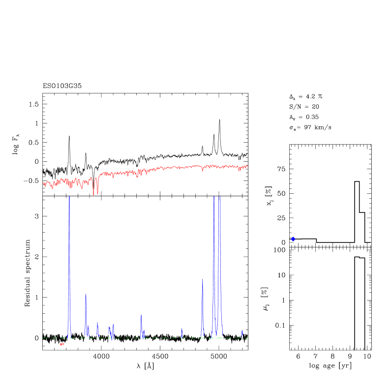
Figure 2: Results of the spectral fits for ESO 103-G35. The top left panel shows the logarithm of the observed and the synthetic spectra (shifted down for clarity). The $O_{\lambda}-M_{\lambda}$ residual spectrum is shown in the bottom left panel. Spectral regions actually used in the synthesis are plotted with a thick line, while masked regions are plotted with a thin line. Crosses indicate points excluded from the synthesis by a 3 sigma clipping algorithm. All spectra are shown in units of the normalization flux $O_{N}$. Panels on the right show the population vector binned in the 10 ages of the base. The top panel corresponds to the population vector in flux fraction ($\vec{x}$), normalized to $\lambda_{0}=4020$ Å, while the corresponding mass fractions vector $\vec{\mu}$ is shown in the bottom. The power-law component $x_{FC}$ is plotted with an (arbitrary) age of $10^{5.5}$ yr and marked by a diamond. No mass is associated to this component (ie, $\mu_{FC}=0$ in the bottom-right panel).

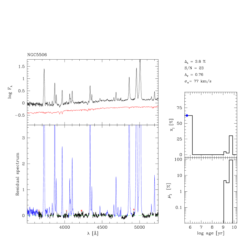
Figure 3: As figure 2, but for NGC 5506

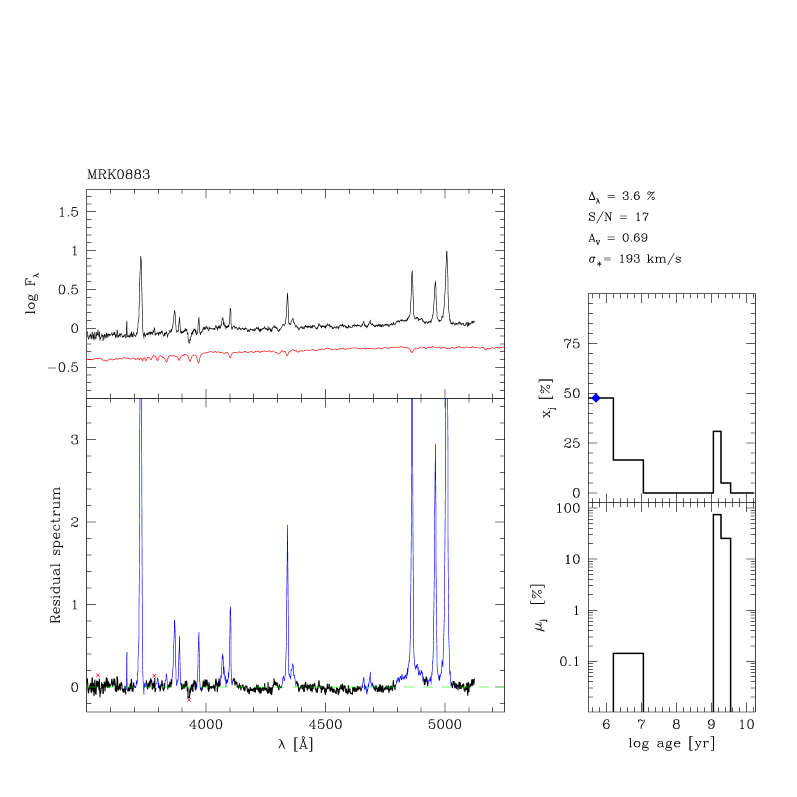
Figure 4: As figure 2, but for Mrk 883.

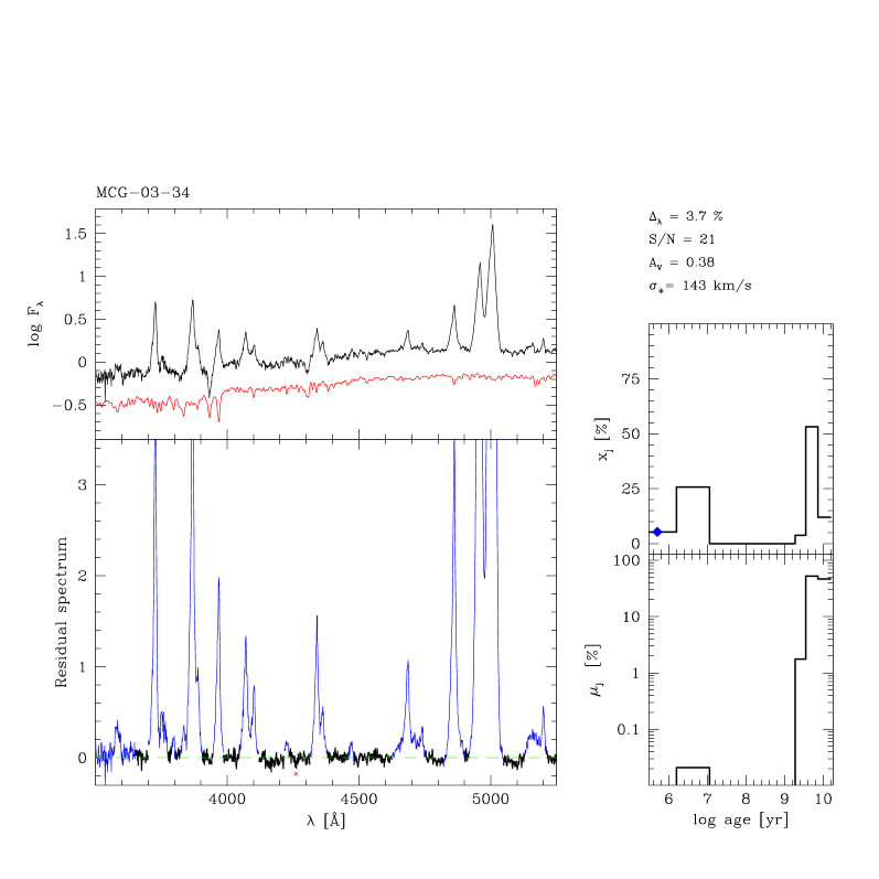
Figure 5: As figure 2, but for MGC -03-034.

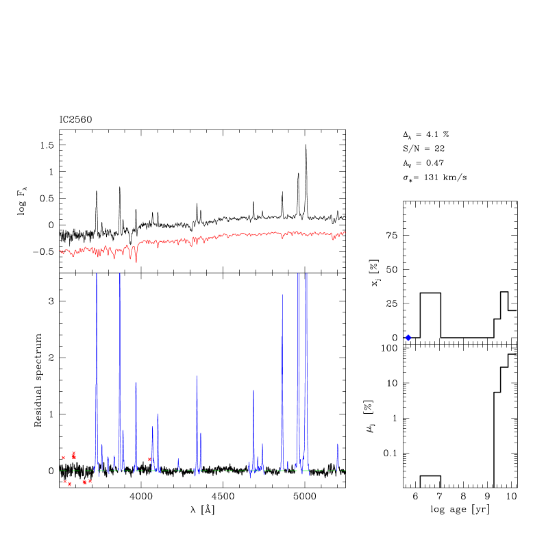
Figure 6: As figure 2, but for IC 2560.

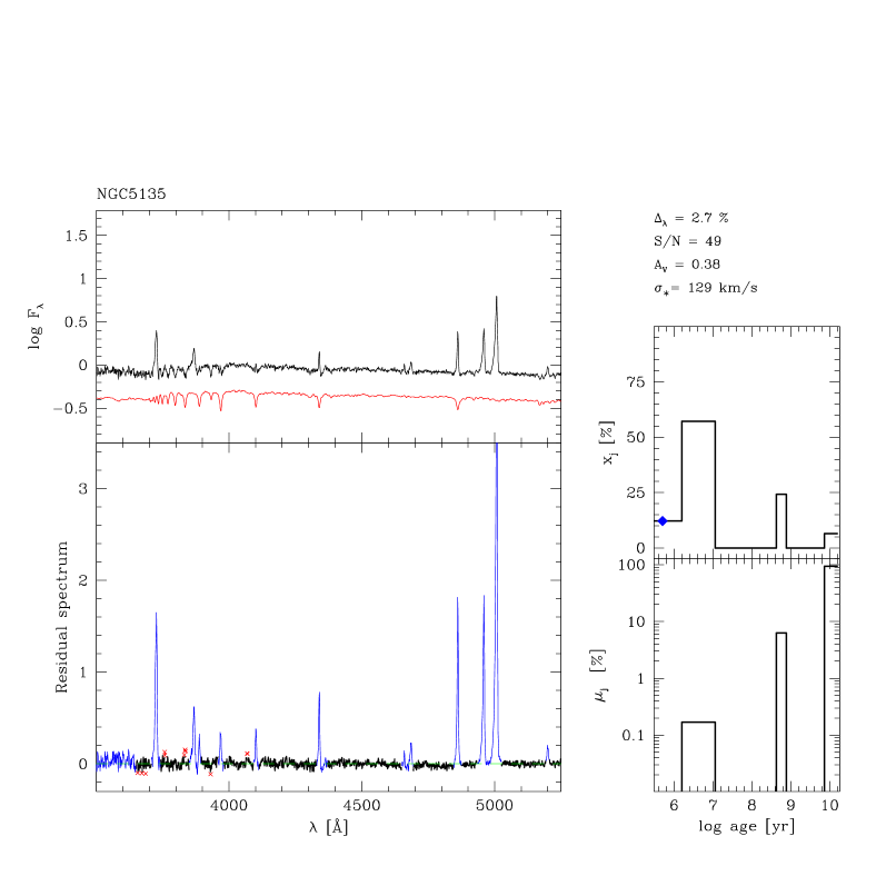
Figure 7: As figure 2, but for NGC 5135.

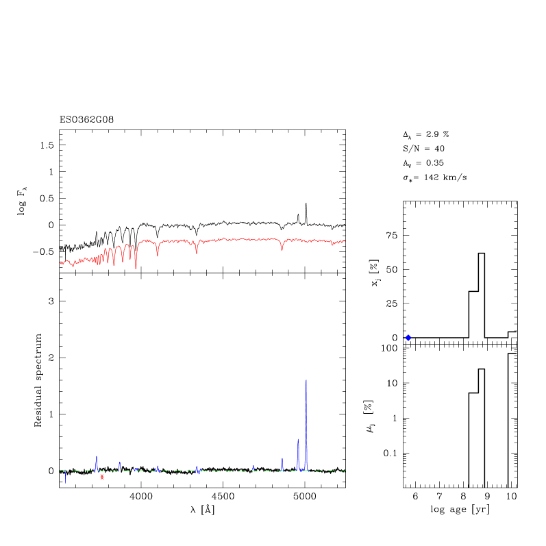
Figure 8: As figure 2, but for ESO 362-G08.

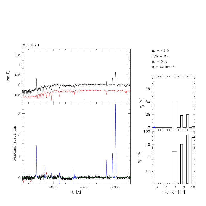
Figure 9: As figure 2, but for Mrk 1370.

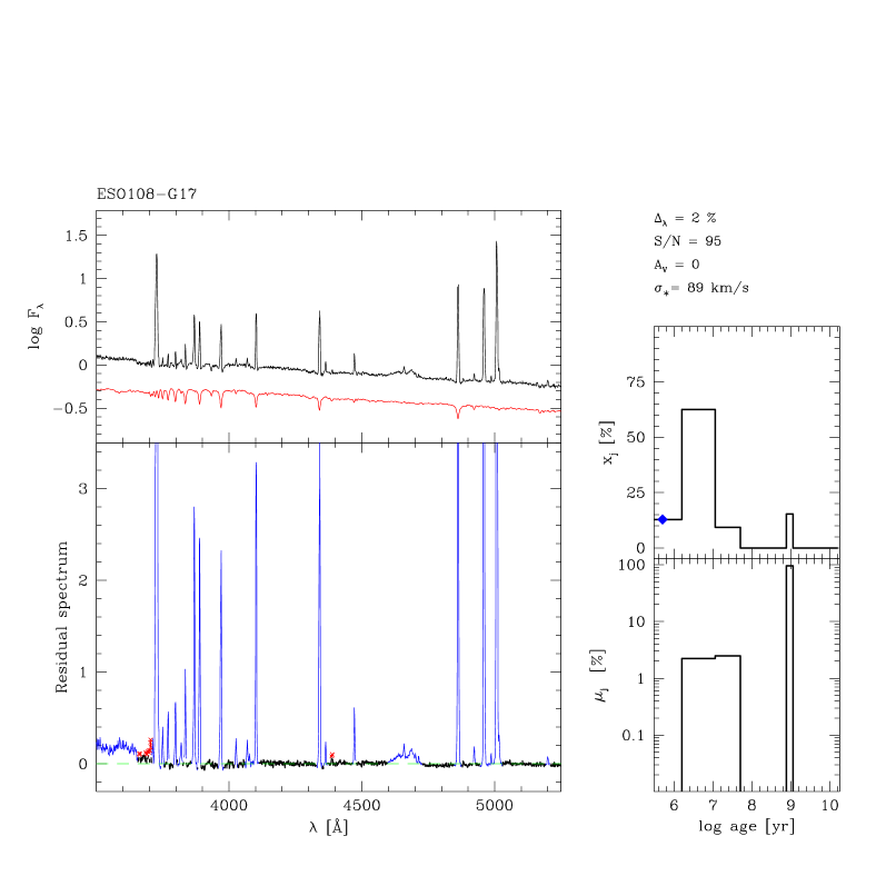
Figure 10: As figure 2, but for the WR galaxy ESO 108-G17.

Figure 11: Comparison of the stellar velocity dispersions estimated by our synthesis method and values compiled from the literature. The identity line is traced by the dashed line, while dotted lines indicate the $\pm 1$ sigma dispersion.

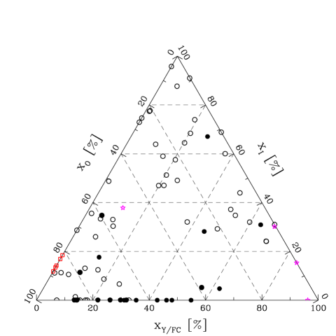
Figure 12: Results of the spectral synthesis condensed on a ($x_{Y/FC},x_{I},x_{O}$) description and plotted in a face on projection of the $x_{Y/FC}+x_{I}+x_{O}=1$ plane. Squares denote normal galaxies and the stars mark starburst galaxies. AGN (mostly Seyfert 2s) are plotted with circles. Filled circles indicate objects in which broad lines have been identified either in direct or polarized light.

4.6 Comparison with previous results

Several galaxies in our sample had their stellar populations studied before. In this section we compare our results with those reported by CF01, who combines observations of Seyfert 2s from several other papers (Heckman et al. 1997; Storchi-Bergmann et al. 1998; Schmitt et al. 1999; González Delgado et al. 1998; 2001). There are 13 galaxies in common with CF01. Their data are similar in wavelength range and quality to those in this paper. Furthermore (not coincidentally, of course), they follow a description of stellar population plus FC components based on three broad groups, similar to those defined in §3.2 and 4.4, which facilitates comparison with our results. The main differences between these two studies resides in the method to analyze the stellar population mixture. Whereas we make use of the full spectrum, the population synthesis performed by CF01 is based in a handful of spectral indices (those listed in Table 3). Also, the stellar population base used by CF01 is that of Schmidt et al. (1991), built upon integrated spectra of star clusters whose age and metallicity were determined by Bica & Alloin (1986), whereas here we use the BC03 models. Notwithstanding the different methodologies, as well as differences in the spectra themselves (eg, due to the larger apertures in CF01), one expects to find a reasonable agreement between these two studies.

Figure 13 summarizes the results of this comparison. Stars are used to plot the $x_{Y/FC}$ fraction of CF01 (called just “$x_{FC}$” in that paper) against our estimate, after re-scaling it to $\lambda_{0}=4861$ Å to match the normalization in CF01. The agreement is very good, with a mean offset of 4% and rms of 6% between the two studies. Crosses and circles are used for the $x_{INT}$ and $x_{OLD}$ components of CF01, which represent $\sim 100$ Myr and $\ga 1$ Gyr age bins. While qualitatively similar, these two components do not compare well with our definitions of $x_{I}$ and $x_{O}$, which are systematically larger and smaller than $x_{INT}$ and $x_{OLD}$ respectively. This is essentially due to the different age-grouping schemes employed. Binning our 100 and 290 Myr base components into $x_{I}^{\prime}$ and all $t\geq 640$ Myr components into $x_{O}^{\prime}$ yields a good correspondence with the $x_{INT}$ and $x_{OLD}$ of CF01, with residuals similar to those obtained for $x_{Y/FC}$, as shown in figure 13.

The two discrepant crosses in the bottom of figure 13 are IC 5135 (= NGC 7130) and NGC 5135. Again, the disagreement is only apparent. Our spectral synthesis find null contributions of the 100 and 290 Myr components, but for NGC 5135 it fits 27% of the continuum at 4861 Å as due to the 640 Myr component, while for IC 5135 18 and 21% are associated with 640 and 900 Myr-old bursts respectively. In our discrete base these components are adjacent in age to the 290 Myr one used as the upper limit for $x_{I}^{\prime}$ in the plot, and hence could well be regrouped within an intermediate age component by a slight modification of the age range associated with $x_{I}^{\prime}$, removing the discrepancy. In short, these ambiguities arise primarily because of the different age resolutions employed in the two studies. Finally, we note that our results for these two galaxies compare well with those of González Delgado et al. (2001), who performed a detailed spectral fit of the Balmer absorption lines characteristic of intermediate age populations using their own models (González Delgado, Leitherer & Heckman 1999). For both IC 5135 and NGC 5135 they find $\sim 50$, 40 and 10% contributions (at 4800 Å) of young, intermediate age and old populations respectively, where the intermediate age component is modeled as a combination of 200, 500 and 1000 Myr bursts. Our condensed population vector (at 4861 Å) for these galaxies are $(x_{Y/FC},x_{I},x_{O})=$ (60,40,0) and (56,27,17) respectively.

We thus conclude that the population synthesis results reported here are consistent to within $\Delta x\sim 10\%$ with previous results, which is quite remarkable given differences in data and analysis methods. A clear advantage of our approach with respect to methods like those in CF01 is that we model the full spectrum, which, besides providing more constraints, yields a more detailed understanding of the different components which make up a Seyfert 2 spectrum. This advantage is explored next.

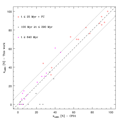
Figure 13: Comparison of the population vector obtained in this work with those in Cid Fernandes et al. (2001a) for 13 Seyfert 2s in common. Different symbols indicate different age ranges. The identity line is traced by the dashed line, while dotted lines indicate the $\pm 10\%$ range.

5 Analysis of the Starlight-subtracted spectra

The excellent fits of the starlight in our spectra provide a unique opportunity to investigate the presence of weak emission features in the $O_{\lambda}-M_{\lambda}$ residual spectra. In this section we explore this opportunity and examine the consequences for the interpretation of the synthesis results.

5.1 Wolf Rayet stars

The presence of WR starts, which produce the so called WR bump at $\sim 4680$ Å, provides a clear indication of starburst activity which is complementary to the population synthesis. We have used the starlight subtracted spectra to investigate the presence of the WR bump in our sample galaxies.

WR stars were detected in the Starburst/WR galaxy ESO108-G17 and in the Seyfert 2s MCG-03-34, Mrk 1210 and NGC 424. Hints of a WR bump are also present in ESO 138-G01 and NGC 4507, but these cases require confirmation either from deeper observations or detection of the 5812 Å feature (Schaerer, Contini & Kunth 1999). These results are presented as notes in Table 2, which summarizes the results of the spectral synthesis models. Galaxies that show WR signatures present important young stellar components (average $x_{Y}$ of 30%), thus validating the results of the synthesis. Given the severe blending with nebular lines of HeII, ArIV, NeIV and FeIII in Seyfert 2s, it is probably futile to attempt any detailed modeling of the WR population.

5.2 Broad emission lines

A close inspection of the starlight subtracted spectra reveals a weak broad H$\beta$ in several of our Seyfert 2s. This is the case of NGC 3035, classified as a Seyfert 1 in NED but reclassified as a Seyfert 2 by J01 on the basis of the absence of broad lines. The top spectrum in figure 14a is the same one used by J01. When we subtract our starlight model, however, a weak but clear broad component emerges in H$\beta$ (bottom spectrum in figure 14a).

Figure 14: (a) Top: Total spectrum of NGC 3035. Bottom: Starlight subtracted spectrum of the same galaxy, showing a broad H$\beta$ component not evident in the total spectrum. The dashed line marks the zero flux level for the bottom spectrum. (b) As the top panel, but for NGC 3660.

At least seven other objects exhibit a similar weak broad component under H$\beta$: ESO 383-G18, MCG-03-34-064, NGC 424, NGC 1068, NGC 3660 (figure 14b), NGC 5506 and NGC 7212, and 2 other objects present marginal evidence for a broad H$\beta$. In principle, these nuclei could be reclassified as Seyfert 1.5 or 1.8, following the notation of Osterbrock (1984). However, the detection of weak broad lines is not per se reason enough to classify a nucleus as of type 1. This violation of the historical definition of Seyfert types by Kachikian & Weedman (1974) is allowed in the context of the unified model, which predicts that a weak BLR should be detected in Seyfert 2s (at least those with a scattering region). We have thus opted not to reclassify these objects, with the understanding that these weak features are probably scattered lines.

The detection of a BLR provides a useful constraint for the interpretation of the spectral synthesis results. Broad emission lines in AGN always come with an associated non-stellar FC, presumably from the nuclear accretion disk. This is true regardless of whether the nucleus and BLR are seen directly, as in bona fide Seyfert 1s, or via scattering, as in NGC 1068, the prototypical Seyfert 2 (Antonucci & Miller 1985). Hence, when the BLR is detected we can be sure that an FC component is also present.

Column 13 of Table 2 lists the spectropolarimetry information available for galaxies in our sample (from the compilation by Gu & Huang 2002 plus new data from Lumsden, Alexander & Hough 2004). The existence of an AGN FC can also be established a priori in Seyfert 2s where spectropolarimetry reveals a type 1 spectrum, ie, those with a “Hidden BLR”. This is the case of 17 objects in our sample. In 7 of these we were able to identify a weak broad H$\beta$ in our direct spectra, while in the remaining cases the BLR detected with the aid of polarimetry is just too faint to be discerned in our data. In these cases, we expect a correspondingly weak FC component. Spectropolarimetry data are available for other fourteen galaxies in our list, but no hidden Seyfert 1 was detected, either because of the absence of an effective mirror or observational limitations. A further alternative is that these are “genuine Seyfert 2s”, ie, AGN with no BLR (Tran 2001, but see Lumsden et al. 2004).

Intriguingly, Tran (2001) reports no BLR detection from his spectropolarimetry data on NGC 3660, while figure 14b leaves no doubt as to the existence of this component in direct light. Variability could be the cause for this discrepancy, in which case this galaxy should be classified as a type 1 Seyfert, because the BLR is seen directly. A type transition of this sort has happened in NGC 7582 (Aretxaga et al. 1999), which suddenly changed spectrum from that of a Seyfert 2 to one with broad emission lines sometime in mid 1998.

Table 2 lists the galaxies for which we have evidence for the presence of weak broad emission lines, either from spectropolarimetry data in the literature (HBLR) or from the present study (BLR). There is a clear tendency for these “broad line Seyfert 2s” (BLS2s) to also show an important FC component in the synthetic spectra. We thus conclude that the synthesis is able to identify a bona fide non-stellar continuum when one is present. Further confirmation of this fact comes from the synthesis of the Seyfert 1 nucleus Mrk 883, which yields $x_{FC}=48\%$. As shown in Paper II (Gu et al. , in preparation), there is also a tendency for BLS2s to have larger [OIII] luminosities. This is consistent with them having more powerful AGN, which, for a fixed scattering efficiency, implies a brighter, easier to detect scattered FC, in agreement with the results reported above.

5.3 FC versus Young Stars

The synthesis also reveals a strong FC component in several objects for which there is no evidence of a BLR. The question then arises of whether $x_{FC}$ corresponds truly to an AGN continuum or to a dusty starburst.

It is hard to distinguish a $F_{\nu}\propto\nu^{-1.5}$ power-law from the spectrum of a reddened young starburst over the wavelength range spanned by our data. The main differences between the spectrum of a 5 Myr SSP seen through $A_{V}\sim 2$–3 mag of dust and this power-law lie in the Balmer absorption lines and in the blue side of the Balmer jump. Since these features are masked in the synthesis, the $x_{FC}$ strength can be attributed to either a dusty-starburst, a true AGN FC, or to a combination of these. This confusion is likely to occur in our synthesis models given that we impose a common $A_{V}$ for all base components while young starbursts are intrinsically rather dusty (Selman et al. 1999).

To illustrate this issue, we note that we obtain $x_{FC}=13\%$ for the WR galaxy ESO 108-G17 (Fig 10). Given that there is no indication of an AGN in this irregular galaxy, it is very likely that this FC component is actually associated with a dusty starburst. The same applies to the starbursting merger NGC 3256, for which we derive $x_{FC}=24\%$. Note, however, that in both cases the synthesis identifies a dominant young population, with $x_{Y}=72$ and 45% respectively.

Not surprisingly, the starburst-FC degeneracy is more pronounced in galaxies known to harbour an active nucleus. For NGC 6221, for instance, we find $x_{FC}=32\%$, $x_{Y}=28\%$ and $A_{V}=0.5$, while from the detailed imaging analysis and modeling of the full spectral energy distribution carried out by Levenson et al. (2001) we know that this nucleus is dominated by heavily extincted ($A_{V}\sim 3$) young star clusters within $<1^{\prime\prime}$ of the AGN, with just a few percent of the optical light originating in the AGN responsible for its Seyfert-like X-ray properties. Most of the large $x_{FC}$ obtained by the synthesis is thus associated with this reddened starburst. Another emblematic example is IC 5135 (NGC 7130), whose UV spectrum shows wind lines of massive stars and a logarithmic slope typical of dusty starbursts, with little or no sign of a power-law (González Delgado et al. 1998), while our synthesis yields $x_{FC}=35\%$, $x_{Y}=34\%$ and $A_{V}=0$. Similar comments can be made about other galaxies in the sample (eg, NGC 5135 and NGC 7582).

These examples show that dusty starbursts, when present, are detected as an FC component by our synthesis method. The fraction $x_{FC}$ should thus be regarded as an upper limit to the contribution of a true FC, while the light fraction associated with very recent star-formation is bracketed between $x_{Y}$ and $x_{Y/FC}$. While there is no way to break this spectral degeneracy without broader spectral coverage, the information on the presence of weak broad lines, collected in Table 2, helps tackling this issue. As discussed in §5.2, whenever a BLR component is detected either in direct or polarized light we can be sure that a true FC is present. One thus expects BLS2s to have larger $x_{FC}$ values than Seyfert 2s for which we have no such independent evidence for the presence of an AGN continuum.

This expectation is confirmed by the synthesis. The four largest values of $x_{FC}$ among Seyfert 2s, for instance, are all found in systems which show weak broad H$\beta$. The link between large $x_{FC}$ and the presence of broad lines is illustrated in figure 15, which shows that the fraction of BLS2s increases systematically with increasing $x_{FC}$. This effect is also clear in the statistics of $x_{FC}$, which assumes a median (mean) value of 21% (19%) among BLS2s but just 2% (7%) among the rest of the Seyfert 2s. As predicted in §5.2, selecting only the galaxies where we see the BLR in our direct spectra increases the median (mean) $x_{FC}$ to 31% (29%), while the ten nuclei where a hidden BLR appears in polarized spectra but not in our data have weaker FCs: 5% (8%).

Overall, these results confirm the prediction of Cid Fernandes & Terlevich (1995), who estimated that a broad component in H$\beta$ should become discernible whenever the scattered FC contributes with $\ga 20$% of the optical continuum. Whenever $x_{FC}$ exceeds $\sim 20\%$ but no BLR is seen, this component most likely originates in a dusty starburst rather than in a non-stellar source.

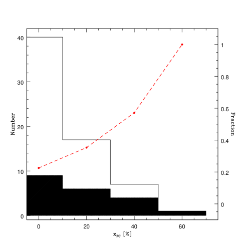
Figure 15: Histogram of the FC fraction in Seyfert 2s. Filled areas correspond to galaxies where a true FC is known to exist from the detection of a BLR in either direct or polarized light. The fraction of these latter galaxies with respect to the whole sample increases with increasing $x_{FC}$, as shown by the dashed line and right-hand scale.

6 Stellar Indices

In order to facilitate the comparison of some relevant aspects of our population synthesis models and published work, we have found it convenient to express our results in terms of specific indices (lines and colours). In this section we present a simple characterization of the stellar populations in Seyfert 2s on the basis of a set of indices commonly used in the literature.

6.1 Direct measurements

In order to provide an empirical characterization of stellar populations in our sample galaxies, we have measured a set of stellar indices directly from the observed spectra. To facilitate the comparison with previous studies, we have employed the index definitions used by Cid Fernandes et al. (2004), which are ultimately based on the studies by Bica & Alloin (1986a,b) and Bica (1988) of star cluster and galaxy spectra.

We have measured the equivalent widths of the Ca II K ($W_{K}$), CN ($W_{CN}$) and G bands ($W_{G}$), as well as the colours $C_{3660}$ and $C_{4510}$, defined as ratios between the continuum at 3660 and 4510 Å to the continuum at 4020 Å, respectively. All these indices are measured with respect to a pseudo continuum, which we define automatically following the recipe in Cid Fernandes et al. (2004), after verifying that it works well for the present sample. Table 3 lists the resulting stellar indices. In this paper we give particular emphasis to the K line. Previous studies have shown that $W_{K}$, which essentially measures the contrast between old and young populations, provides a useful mono-parametric description of stellar populations in galaxies. For instance, Seyfert 2s with unambiguous signatures of recent star-formation (such as UV wind lines, the WR bump, or high order Balmer absorption lines) all have K lines diluted to $W_{K}\la 10$ Å (CF01).

Figure 16a shows the $W_{K}$ versus $C_{3660}$ diagram. This plot has the advantage of involving only direct measurements, which, in the case of the JO1 spectra, is not possible for more popular indices. The solid and dotted curves show the evolution of instantaneous burst BC03 models for solar (solid, green line) and 2.5 solar metallicity (dotted, red). The region occupied by pure stellar populations in this diagram is delimited by these tracks and a mixing line joining the youngest and oldest models. Points located below the BC03 models in the bottom-right of the plot are explained as a combination of observational errors and intrinsic reddening, both of which affect more the $C_{3660}$ colour than $W_{K}$.

The dashed line in figure 16 represents a mixing line, where a canonical AGN $F_{\nu}\propto\nu^{-1.5}$ power-law is added to an old stellar population in different proportions, from a pure power-law at $(W_{K},C_{3660})=(0,1.05)$ to a pure $10^{10}$ yr population at $\sim(20,0.7)$. The fact that few galaxies line up along this mixing line shows that a simple “elliptical galaxy” plus power-law model, adopted in many early AGN studies, does not apply to the bulk of Seyfert 2s. On the contrary, the spread of points in this diagram implies a substantial diversity in the central stellar populations of Seyfert 2s, in agreement with our synthesis results (eg, figure 12) as well as with previous studies (Cid Fernandes, Storchi-Bergmann & Schmitt 1998; J01; Serote Roos et al. 1998; Boisson et al. 2000).

Stellar Indices
Galaxy	$W_{K}$ [Å]	$W_{CN}$ [Å]	$W_{G}$ [Å]	$C_{3660}$	$C_{4510}$
ESO 103G35	16.6$\pm$0.7	10.5$\pm$0.9	10.1$\pm$0.4	0.61$\pm$0.03	1.47$\pm$0.04
ESO 104G11	10.9$\pm$1.3	5.4$\pm$1.7	7.8$\pm$0.7	0.57$\pm$0.05	1.21$\pm$0.06
ESO 137-G34	16.8$\pm$0.7	11.4$\pm$0.9	10.8$\pm$0.4	0.75$\pm$0.04	1.45$\pm$0.04
ESO 138-G01	7.7$\pm$0.5	5.0$\pm$0.7	4.6$\pm$0.4	0.83$\pm$0.02	0.93$\pm$0.02
ESO 269-G12	17.5$\pm$0.9	14.0$\pm$1.0	11.1$\pm$0.5	0.66$\pm$0.04	1.42$\pm$0.04
ESO 323G32	16.3$\pm$0.8	13.8$\pm$0.9	10.7$\pm$0.4	0.55$\pm$0.03	1.39$\pm$0.04
ESO 362G08	8.0$\pm$0.5	8.0$\pm$0.6	7.4$\pm$0.3	0.43$\pm$0.02	1.10$\pm$0.02
ESO 373G29	5.9$\pm$0.5	6.4$\pm$0.7	6.4$\pm$0.4	0.76$\pm$0.02	1.02$\pm$0.02
ESO 381-G08	8.9$\pm$0.4	5.5$\pm$0.5	5.6$\pm$0.2	0.72$\pm$0.01	1.15$\pm$0.02
ESO 383-G18	10.5$\pm$0.8	6.1$\pm$1.1	7.0$\pm$0.6	0.90$\pm$0.04	1.07$\pm$0.04
ESO 428G14	13.5$\pm$0.7	10.7$\pm$0.8	9.2$\pm$0.4	0.60$\pm$0.03	1.24$\pm$0.03
ESO 434G40	16.7$\pm$0.7	13.5$\pm$0.9	11.0$\pm$0.4	0.64$\pm$0.03	1.52$\pm$0.04
Fai 0334	9.8$\pm$1.8	7.5$\pm$1.9	8.6$\pm$0.9	0.73$\pm$0.07	1.19$\pm$0.06
Fai 0341	13.7$\pm$1.2	10.0$\pm$1.3	10.5$\pm$0.6	0.73$\pm$0.05	1.49$\pm$0.06
IC 1657	10.9$\pm$1.4	7.4$\pm$1.7	8.9$\pm$0.8	0.66$\pm$0.06	1.31$\pm$0.07
IC 2560	11.0$\pm$1.0	11.0$\pm$1.1	9.6$\pm$0.5	0.76$\pm$0.04	1.40$\pm$0.05
IC 5063	16.9$\pm$0.7	12.4$\pm$0.8	10.5$\pm$0.4	0.61$\pm$0.04	1.47$\pm$0.04
IC 5135	4.6$\pm$0.4	3.4$\pm$0.5	3.2$\pm$0.3	0.88$\pm$0.02	0.92$\pm$0.01
IRAS 11215	14.3$\pm$0.7	9.0$\pm$1.0	9.1$\pm$0.4	0.62$\pm$0.03	1.26$\pm$0.04
MCG +01-27	7.8$\pm$0.7	8.2$\pm$0.8	7.4$\pm$0.4	0.55$\pm$0.03	1.05$\pm$0.03
MCG -03-34	11.9$\pm$1.5	12.3$\pm$1.7	9.1$\pm$0.9	0.80$\pm$0.06	1.35$\pm$0.07
MRK 0897	4.8$\pm$0.4	4.1$\pm$0.5	4.1$\pm$0.3	0.70$\pm$0.01	0.93$\pm$0.01
MRK 1210	9.0$\pm$1.5	8.7$\pm$1.9	6.5$\pm$1.0	0.79$\pm$0.06	1.18$\pm$0.07
MRK 1370	5.8$\pm$0.8	7.2$\pm$0.9	6.1$\pm$0.4	0.53$\pm$0.02	1.05$\pm$0.03
NGC 0424	11.1$\pm$0.6	9.5$\pm$0.7	7.8$\pm$0.4	0.86$\pm$0.03	1.33$\pm$0.03
NGC 0788	17.9$\pm$0.8	13.2$\pm$1.0	11.2$\pm$0.5	0.68$\pm$0.03	1.37$\pm$0.04
NGC 1068	8.6$\pm$0.5	8.9$\pm$0.7	6.5$\pm$0.4	0.86$\pm$0.02	1.14$\pm$0.02
NGC 1125	10.5$\pm$1.0	8.4$\pm$1.2	7.9$\pm$0.5	0.63$\pm$0.03	1.14$\pm$0.04
NGC 1667	18.9$\pm$1.0	15.3$\pm$1.2	11.7$\pm$0.6	0.67$\pm$0.04	1.46$\pm$0.06
NGC 1672	10.0$\pm$0.6	7.9$\pm$0.8	6.8$\pm$0.4	0.63$\pm$0.02	1.08$\pm$0.02
NGC 2110	13.7$\pm$1.0	14.2$\pm$1.1	10.5$\pm$0.5	0.74$\pm$0.05	1.40$\pm$0.05
NGC 2979	11.4$\pm$0.9	8.5$\pm$1.1	8.7$\pm$0.5	0.51$\pm$0.03	1.29$\pm$0.04
NGC 2992	16.4$\pm$0.8	14.2$\pm$0.8	11.2$\pm$0.4	0.51$\pm$0.04	1.57$\pm$0.04
NGC 3035	12.9$\pm$0.6	11.5$\pm$0.7	9.1$\pm$0.3	0.68$\pm$0.03	1.32$\pm$0.03
NGC 3081	15.1$\pm$0.9	13.6$\pm$1.0	9.4$\pm$0.5	0.78$\pm$0.04	1.44$\pm$0.05
NGC 3281	16.0$\pm$1.1	12.5$\pm$1.3	11.6$\pm$0.6	0.70$\pm$0.05	1.73$\pm$0.07
NGC 3362	15.3$\pm$0.8	11.3$\pm$0.9	9.5$\pm$0.5	0.61$\pm$0.03	1.39$\pm$0.04
NGC 3393	17.4$\pm$0.7	14.6$\pm$0.8	10.6$\pm$0.4	0.71$\pm$0.03	1.44$\pm$0.04
NGC 3660	7.2$\pm$0.7	8.0$\pm$0.8	6.4$\pm$0.4	0.78$\pm$0.03	1.26$\pm$0.03
NGC 4388	14.0$\pm$1.0	9.3$\pm$1.2	9.4$\pm$0.5	0.77$\pm$0.04	1.43$\pm$0.05
NGC 4507	11.1$\pm$0.4	8.8$\pm$0.6	7.4$\pm$0.3	0.81$\pm$0.04	1.20$\pm$0.02
NGC 4903	17.6$\pm$0.9	15.1$\pm$1.0	12.0$\pm$0.4	0.67$\pm$0.04	1.71$\pm$0.06
NGC 4939	17.3$\pm$0.9	14.3$\pm$1.0	11.8$\pm$0.5	0.72$\pm$0.04	1.54$\pm$0.05
NGC 4941	17.9$\pm$0.8	15.3$\pm$1.0	11.3$\pm$0.5	0.65$\pm$0.03	1.58$\pm$0.05
NGC 4968	10.7$\pm$1.0	7.8$\pm$1.2	8.1$\pm$0.5	0.52$\pm$0.04	1.29$\pm$0.05
NGC 5135	3.3$\pm$0.4	3.7$\pm$0.5	3.8$\pm$0.3	0.77$\pm$0.02	0.89$\pm$0.01
NGC 5252	17.0$\pm$0.6	13.5$\pm$0.7	11.0$\pm$0.3	0.71$\pm$0.02	1.43$\pm$0.03
NGC 5427	16.4$\pm$0.9	13.1$\pm$1.1	11.4$\pm$0.5	0.67$\pm$0.04	1.33$\pm$0.05
NGC 5506	7.9$\pm$1.0	5.8$\pm$1.1	5.7$\pm$0.5	0.93$\pm$0.05	1.29$\pm$0.04
NGC 5643	9.7$\pm$0.5	6.3$\pm$0.6	6.3$\pm$0.3	0.54$\pm$0.02	1.09$\pm$0.02
NGC 5674	12.4$\pm$1.1	11.3$\pm$1.3	7.9$\pm$0.6	0.65$\pm$0.04	1.28$\pm$0.05
NGC 5728	11.7$\pm$0.5	9.3$\pm$0.6	7.8$\pm$0.3	0.60$\pm$0.02	1.16$\pm$0.02
NGC 5953	11.7$\pm$0.5	8.3$\pm$0.6	7.1$\pm$0.3	0.58$\pm$0.02	1.24$\pm$0.02
NGC 6221	6.9$\pm$0.5	2.1$\pm$0.6	2.7$\pm$0.3	0.78$\pm$0.02	1.05$\pm$0.02
NGC 6300	16.6$\pm$1.2	9.9$\pm$1.4	9.5$\pm$0.7	0.58$\pm$0.04	1.58$\pm$0.07
NGC 6890	13.7$\pm$0.8	7.9$\pm$1.0	8.9$\pm$0.5	0.68$\pm$0.03	1.42$\pm$0.04
NGC 7172	16.7$\pm$1.3	13.0$\pm$1.4	10.8$\pm$0.6	0.53$\pm$0.05	1.56$\pm$0.07
NGC 7212	12.0$\pm$0.6	8.2$\pm$0.8	8.0$\pm$0.4	0.84$\pm$0.03	1.44$\pm$0.03
NGC 7314	17.8$\pm$1.9	11.7$\pm$2.5	10.0$\pm$1.1	0.67$\pm$0.09	1.37$\pm$0.11
NGC 7496	4.1$\pm$0.4	3.4$\pm$0.5	3.8$\pm$0.2	0.78$\pm$0.01	0.94$\pm$0.01
NGC 7582	4.5$\pm$0.4	1.6$\pm$0.5	3.0$\pm$0.2	0.59$\pm$0.01	1.18$\pm$0.01
NGC 7590	16.3$\pm$0.7	10.2$\pm$0.9	10.2$\pm$0.4	0.59$\pm$0.03	1.51$\pm$0.04
NGC 7679	2.1$\pm$0.6	2.2$\pm$0.6	2.7$\pm$0.3	0.55$\pm$0.01	0.89$\pm$0.01
NGC 7682	16.3$\pm$0.9	13.1$\pm$1.1	10.2$\pm$0.5	0.73$\pm$0.04	1.43$\pm$0.05
NGC 7743	13.6$\pm$0.7	8.5$\pm$0.8	8.2$\pm$0.4	0.54$\pm$0.02	1.27$\pm$0.03
MRK 0883	6.2$\pm$0.5	5.1$\pm$0.7	2.7$\pm$0.3	0.82$\pm$0.02	1.10$\pm$0.02
NGC 1097	5.1$\pm$0.5	5.3$\pm$0.7	5.2$\pm$0.3	0.74$\pm$0.02	0.99$\pm$0.02
NGC 4303	11.8$\pm$0.6	8.7$\pm$0.7	7.4$\pm$0.3	0.64$\pm$0.02	1.22$\pm$0.03
NGC 4602	9.6$\pm$0.7	7.6$\pm$1.0	8.1$\pm$0.5	0.59$\pm$0.03	1.11$\pm$0.03
NGC 7410	3.3$\pm$0.4	3.7$\pm$0.5	3.8$\pm$0.3	0.75$\pm$0.02	0.92$\pm$0.01
ESO 108-G17	2.4$\pm$0.6	1.4$\pm$0.9	2.2$\pm$0.5	1.06$\pm$0.03	0.81$\pm$0.02
NGC 1487	2.0$\pm$0.7	4.5$\pm$1.1	3.4$\pm$0.6	0.86$\pm$0.03	0.69$\pm$0.02
NGC 2935	12.8$\pm$0.6	11.5$\pm$0.7	9.8$\pm$0.3	0.61$\pm$0.02	1.33$\pm$0.03
NGC 3256	3.6$\pm$0.5	1.7$\pm$0.6	2.8$\pm$0.3	0.77$\pm$0.02	0.89$\pm$0.01
NGC 2811	18.6$\pm$0.6	18.2$\pm$0.7	12.7$\pm$0.3	0.57$\pm$0.02	1.57$\pm$0.03
NGC 3223	17.2$\pm$0.7	15.6$\pm$0.8	12.2$\pm$0.4	0.63$\pm$0.03	1.59$\pm$0.04
NGC 3358	18.4$\pm$0.7	15.9$\pm$0.8	11.8$\pm$0.4	0.61$\pm$0.03	1.56$\pm$0.04
NGC 3379	19.0$\pm$0.6	18.6$\pm$0.6	12.5$\pm$0.3	0.59$\pm$0.02	1.49$\pm$0.03
NGC 4365	18.6$\pm$0.5	18.5$\pm$0.6	12.2$\pm$0.3	0.54$\pm$0.02	1.56$\pm$0.03

Table 3: Spectral indices, computed with the definitions of Cid Fernandes et al. (2004). Colours were corrected for Galactic extinction.

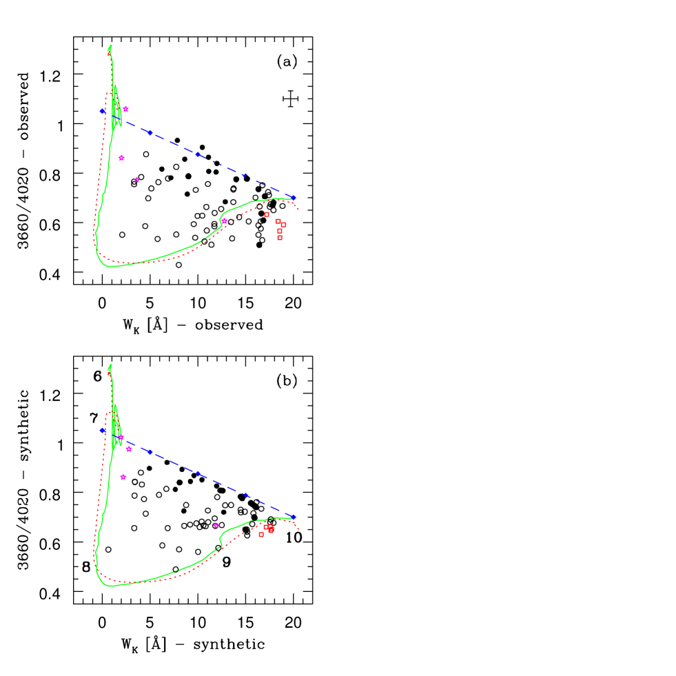
Figure 16: $C_{3660}$ versus $W_{K}$ diagram for the J01 sample. Panel (a) shows the results for $C_{3660}$ and $W_{K}$ as measured directly from the observed spectra, whereas in (b) these two indices are measured from synthetic spectra constructed to match the observed stellar spectrum. In both panels the solid (green) and dotted (red) curves represent the evolution of BC03 models of instantaneous bursts with $Z_{\odot}$ and $2.5Z_{\odot}$ metallicity respectively. The approximate location of populations with ages $\log t=6$, 7 , 8 , 9 and 10 yr are indicated by the labels in panel (b). The dashed (blue) line between $(W_{K},C_{3660})=(0,1.05)$ and $\sim(20,0.7)$ represents a mixing line, where a $F_{\nu}\propto\nu^{-1.5}$ power-law is added to a $10^{10}$ yr stellar population; diamonds mark power-law fractions in steps of 25%. The average error bar is indicated in the top-right in (a). Symbols as in figure 12.

6.2 Indirect measurements

Unfortunately, other useful tracers of the star-formation history such as the $D_{n}(4000)$ and H$\delta_{A}$ indices (Balogh et al. 1999; Worthey & Otaviani 1997), cannot be measured directly for many of our galaxies because of severe contamination by emission lines. An indirect measurement of these indices can be performed over the model starlight spectra described in §3. Naturally, the information contained in these “semi-empirical” indices is identical to the one contained in the model spectra from which they are measured. They are nevertheless useful for stellar population diagnostics based on observable indices, such as the $D_{n}(4000)$ versus H$\delta_{A}$ diagram amply explored by Kauffmann et al. (2002, 2003) in their study of SDSS galaxies.

Figure 16b shows $W_{K}$ and $C_{3660}$ measured from the deredenned synthetic spectra. The main difference with respect to the observed version of this diagram (figure 16a) is in the bottom-right points, which move upwards (to within the region spanned by the BC03 models) due to the correction for intrinsic reddening. Objects in which a BLR is detected either in direct or polarized light (ie, BLS2s, represented by filled circles) occupy a characteristic region in this plot, close to the power-law + old stars mixing line. This is consistent with the existence of an FC implied by the detection of a BLR. This tendency is also evident, albeit less clear, in the observed $W_{K}$-$C_{3660}$ diagram (figure 16a).

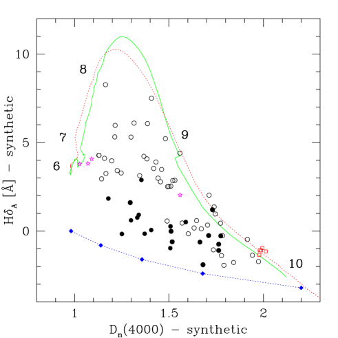
Figure 17: $D_{n}(4000)$ versus H$\delta_{A}$ diagram. As in Figure 16b, both indices were measured from the synthetic spectra. The numbers around the BC03 SSP evolutionary sequences mark the logarithm of the age (in yr). Symbols and lines as in figure 16.

Figure 17 shows the synthetic $D_{n}(4000)$-H$\delta_{A}$ diagram for our sample. As in figure 16, the scatter of points in this plot reflects the wide variety of stellar populations of Seyfert 2s, ranging from systems dominated by young stars, to post-starbursts and older systems, as well as mixtures of these populations. Again, objects where an FC is known to be present from the detection of a BLR are systematically off-set towards the power-law + old stars mixing line. Note, however, that even these objects cannot be entirely explained in terms of this simple two-components model. An illustrative example in this respect is Mrk 1210, with $D_{n}(4000)=1.3$ and H$\delta_{A}=1.6$ Å. This galaxy has both a hidden BLR detected through spectropolarimetry (Tran, Miller & Kay 1992) and a very young starburst, responsible for its WR bump (Storchi Bergmann, Cid Fernandes & Schmitt 1998; Joguet 2001). Other examples include Mrk 477 (Heckman et al. 1997; Tran et al. 1992), Mrk 463E (González-Delgado et al. 2001; Miller & Goodrich 1990) and NGC 424 (Moran et al. 2000; Joguet 2001).

7 Discussion

7.1 Statistics of star-formation in Seyfert 2s

Figure 18 shows histograms of the $x_{Y/FC}$, $x_{I}$ and $x_{O}$ components for the 65 Seyfert 2s in the sample, as well as the distributions of $W_{K}$ and $\overline{\log t}$, the flux weighted mean stellar age (computed according to its definition in Cid Fernandes, Rodrigues Lacerda & Leão 2003). These histograms illustrate the frequency of recent star-formation in Seyfert 2s.

There are several possible definitions of “recent star-formation”, either in terms of observed quantities or model parameters. For instance, 31% of the objects have $W_{K}<10$ Å, a rough dividing line between composite starburst + Seyfert 2 systems and those dominated by older populations according to CF01. This frequency increases to 51% using a $W_{K}<12$ Å cut. In terms of $x_{Y/FC}$, we find that nearly half (46%) of the sample has $x_{Y/FC}>20\%$, while for about one-third this fraction exceeds 30%. Old stars, although present in all galaxies, only dominate the light ($x_{O}>70\%$) in 31% of the cases. In terms $\overline{\log t}$, we find that 25 out of our 65 galaxies (38%) have $\overline{\log t}<8.5$, ie, mean ages smaller than 300 Myr. In summary, depending on the criterion adopted, between 1/3 and 1/2 of Seyfert 2s have experienced significant star-formation in the past few hundred Myr. These numbers are similar to those derived by J01 by means of a visual characterization of stellar populations for the same sample and with those obtained by Storchi-Bergmann et al. (2001) for a sample $\sim$ half as big as ours.

Naturally, one would like to compare the incidence of recent star-formation in Seyfert 2s to that in other types of nuclei. A particularly interesting comparison to be made is that between Seyfert 2s and LINERs, given that these two classes were once thought to belong to the same family (Ferland & Netzer 1983; Halpern & Steiner 1993). We have too few LINERs in our sample to perform this comparison, but we may borrow from the results of Cid Fernandes et al. (2004) and González Delgado et al. (2004), who have recently surveyed the stellar populations of LINERs and LINER/HII Transition Objects using spectroscopic data practically identical to the one used in this paper and a similar method of analysis. Their results are very different from ours. For instance, while we find that over 2/3 of Seyfert 2s have $x_{Y/FC}>10\%$, most LINERs have $x_{Y/FC}<10\%$, and are often dominated by old stars. Still according to these authors, a large fraction of Transition Objects harbour significant numbers of $10^{8}$–$10^{9}$ yr stars, similar to those found in $x_{I}$-dominated Seyfert 2s (eg, ESO 362-G08 and Mrk 1370, figures 8 and 9). Their $x_{Y/FC}$ strength, however, is only 6% on average, compared to 23% for our Seyfert 2s.

Thus, a substantial fraction of nearby Seyfert 2s live in much younger stellar environments than LINERs or Transition Objects, which suggests an evolutionary sequence. Given that the later objects are known to harbour less luminous AGN and have different gas excitation conditions than Seyferts, if confirmed, this would imply a substantial evolution of the AGN itself—in parallel with the evolution of stars in its surroundings.

Figure 18: Distributions of the $x_{Y/FC}$, $x_{I}$ and $x_{O}$ fractions, $W_{K}$ and the flux weighted mean stellar age inferred from the synthesis. Only Seyfert 2s were included in these histograms.

7.2 Aperture effects

Spectra collected through apertures of fixed angular size sample distance-dependent linear scales, which may introduce systematic effects on the derived stellar population mixtures. In order to investigate whether such potential biases affect our results in some systematic way we plot in figure 19 the equivalent width of CaII K against the pc/arcsec scale. (Recall that our observations cover an area of $\sim 1$ arcsec².) No systematic trend is observed between this stellar population tracer and the linear dimension of the regions sampled by our data. The same conclusion holds for the $\vec{x}$ components, none of which correlates with distance either. The absence of systematic trends indicates that our analysis is not affected by aperture effects.

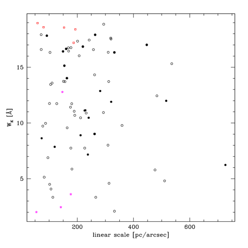
Figure 19: Projected linear scale against the equivalent width of CaII K. Symbols as in figure 12.

7.3 Relation to host galaxy morphology

A galaxy’s morphology carries important information for the study of star formation history in galaxies (eg., Kennicutt 1998). From early to late types, galaxy colours become bluer and star formation rates higher. Storchi-Bergmann et al. (2001) studied the relationship between nuclear stellar population and morphology in a sample of 35 Seyfert 2s, 13 in common with our sample. They found that the fraction of galaxies with recent nuclear/circumnuclear starburst increases along the Hubble sequence and that there is a relation between the presence of a nuclear starburst and a late “inner Hubble type” from the HST classifications of Malkan, Gorjian & Tam (1998).

In order to check this result in our larger sample, we have collected morphological information on the host galaxies from RC3, and the inner Hubble types from Malkan et al. (1998). In figure 20 we plot three of our stellar population tracers (W_K, x_Y/FC, and mean age) against the RC3 and inner morphological types (later types have larger numbers). There is no correlation in our sample between (optical) morphology and nuclear star formation. Since the HST snapshot survey of Malkan et al. (1998) was taken using the F606W filter which is sensitive to dust extinction and H$\alpha$ emission, we searched the HST/NICMOS archive data and found images for 36 of our galaxies taken with the F160W filter. No clear trend between morphological type and nuclear stellar population is found in the near-IR images either.

Finally, following Storchi-Bergmann et al. we also looked for companions to our Seyfert 2s according to angular separation, radial velocity, and apparent magnitude. We find that 40% of the galaxies with $W_{K}<10$ Å and 47% of those with $W_{K}>10$ Å show the presence of companions, compared respectively with 42% and 47% that do not have near neighbours.

Hence, contrary to the findings of Storchi-Bergmann et al. (2001) we find no correlation between the nuclear stellar populations of Seyfert 2 galaxies and either morphological types or environments. Since there is a substantial overlap between our samples, the discrepancy is most likely statistical. Given the importance of the result, however, it would be worthwhile to repeat the study in an even larger sample of galaxies.

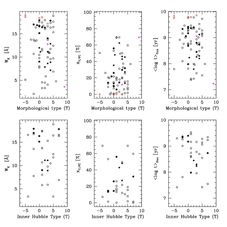
Figure 20: Distribution of morphological Hubble type for the host galaxies (top panels) and the inner region (bottom panels) against stellar population properties: W_K (left), $x_{Y/FC}$ (middle) and the mean age (right). Symbols as in figure 12.

8 Summary

We have presented a study of the stellar population in the central $\sim 50$–500 pc of a large, well defined and homogeneous sample of Seyfert 2s from the atlas of J01. Our main results may be summarized as follows:

1. We have developed a spectral synthesis code which decomposes an observed spectrum as a sum of simple stellar populations, represented by state-of-the-art evolutionary synthesis models, plus an AGN continuum. Unlike previous studies, which use only a few absorption equivalent widths and colours (eg Bica 1988; Schmitt et al. 1999; Cid Fernandes et al. 2001a,b), we now synthesize the whole observed spectrum. The method produces an estimate of the star-formation history in terms of flux ($\vec{x}$) or mass ($\vec{\mu}$) fractions associated to each component in the spectral base, as well as extinction and velocity dispersions. As in other population synthesis studies, the accuracy of our method is limited by noise, spectral coverage, and intrinsic degeneracies of stellar populations. These limitations are not critical as long as one does not attempt an over-detailed description of the SFH.

2. The synthesis method was applied to 3500–5200 Å spectra of 65 Seyfert 2s and 14 other galaxies from the J01 atlas. The synthesis produces excellent fits of the observed spectra, with typical flux residuals of 2–5%. The star formation history deduced from these fits is remarkably varied among Seyfert 2s. Young starbursts, intermediate age, and old populations all appear in significant and mixed amounts.

3. The stellar velocity dispersions obtained from the synthesis are in good agreement with measurements in the literature for galaxies in common. This is important since this information gives us a handle on the black-hole mass (Ferrarese & Merrit 2000; Gebhart et al. 2000).

4. The starlight-subtracted spectra were used to investigate the presence of weak broad emission features which are hard to detect in the total spectrum. This analysis revealed the signatures of WR stars in 3 (maybe 5) Seyfert 2s, all of which have large young stellar populations as deduced by the synthesis.

5. The analysis of the “pure-emission” spectra further allowed the detection of a weak BLR-like component under H$\beta$ in several Seyfert 2s. For most of these objects independent spectropolarimetry data reveals a type 1 spectrum. We are thus detecting in direct, non-polarized light the scattered BLR predicted by the unified model.

6. The detection of a BLR either in direct or polarized light implies that an associated FC should also be present in our spectrum. Indeed, the FC strengths obtained by the spectral decomposition for the 17 Seyfert 2s in our sample which present such evidence are substantially larger than for nuclei with no indications of a BLR. The fraction of these “broad line Seyfert 2s” increases systematically with increasing $x_{FC}$.

7. Dusty young starbursts can also appear disguised as an AGN-looking continuum. We have identified several cases where this indeed happens. These Seyfert 2s tend to have large $x_{FC}$ and $x_{Y}$ fractions. The information on the existence of a BLR, and thus of a true FC component, helps breaking, at least partly, this starburst-FC degeneracy. Whenever the spectral synthesis identifies a strong ($\ga 20\%$) FC but no BLR is detected either in the residual or polarized spectra, the FC is most likely dominated by a dusty starburst rather than scattering of a hidden AGN.

8. Stellar indices were measured both from the observed and synthetic spectra to provide a more empirical characterization of the stellar content of our galaxies and facilitate comparisons with independent studies. These indices, which include $W_{K}$, the 3660/4020 colour, $D_{n}(4000)$ and H$\delta_{A}$, confirm the heterogeneity of nuclear stellar populations in Seyfert 2s.

9. Between 1/3 and 1/2 of nearby Seyfert 2s have experienced significant star formation in the recent past. Thus, as a class, Seyfert 2 nuclei live in a much younger stellar environment than LINERs and normal galactic nuclei.

10. We find no significant correlation between the host morphology (as deduced both from ground based and HST optical and near-IR images) and stellar population in Seyfert 2s. The presence of companions does not seem to correlate with the stellar populations either.

We have shown that using modern population synthesis models it is possible to obtain meaningful information about the history of star formation in objects for which the spectral data are dominated by strong emission lines. The road to detailed quantitative investigations of the relationship between star-formation and AGN is now open. We will be traveling along it in our forthcoming papers.

References

- [] Antonucci R., 1993, ARA&A, 31, 473
- [] Antonucci R., Miller J.S., 1985, ApJ, 297, 621
- [] Aretxaga I., Terlevich E., Terlevich R., Cotter G., Diaz A., 2001, MNRAS, 325, 636
- [] Aretxaga I., Joguet B., Kunth D., Melnick J., Terlevich R., 1999, ApJ, 519, L123
- [] Balogh, M. L., Morris, S. L., Yee, H. K. C., Carlberg, R. G., & Ellingson, E. 1999, ApJ, 527, 54
- [] Bica E., Alloin D.,1986, A&A, 162, 21
- [] Boisson C., Joly M., Moultaka J., Pelat D., Serote Roos M., 2000, A&A, 357, 850
- [] Bruzual G., Charlot S., 2003, MNRAS, 344, 1000
- [] Cardelli J. A., Clayton G. C., Mathis J.S., 1989, ApJ, 345, 245
- [] Chabrier G., 2003, PASP, 115, 763
- [Chan, Mitchell, & Cram(2003)] Chan, B. H. P., Mitchell, D. A., & Cram, L. E. 2003, MNRAS, 338, 790
- [] Cid Fernandes R., Terlevich R., 1995, MNRAS, 272, 423
- [] Cid Fernandes R., Storchi-Bergmann T., Schmitt H. R., 1998, MNRAS, 297, 579
- [] Cid Fernandes, R., Heckman, T., Schmitt, H., Gonzalez Delgado, R. M., & Storchi-Bergmann, T. 2001a, ApJ, 558, 81
- [] Cid Fernandes R., Sodré L., Schmitt H. R., Leão J. R. S., 2001b, MNRAS, 325, 60
- [] Cid Fernandes R., Leao J. Lacerda R. R., 2003, MNRAS, 340, 29
- [] Cid Fernandes R., González Delgado R. M., Schmitt H., Storchi-Bergmann T., Pires Martins L., Pérez E., Heckman T., Leitherer C., Schaerer D. 2004, ApJ, 605, 105
- [] Colina L., Gonzalez Delgado R., Mas-Hesse J. M., Leitherer C., 2002, ApJ, 579, 545
- [] Colina L., Cervino, M., Gonzalez Delgado, R.M. , 2003, ApJ, 593, 127
- [] Della Ceca R., Pellegrini S., Bassani L., et al., 2001, A&A, 375, 781
- [] Dessauges-Zavadsky M., Pindao M., Maeder A., Kunth D., 2000 A&A, 355, 89
- [] de Vaucouleurs G., de Vaucouleurs A., Corwin H.G., Buta R.J., Paturel G., Fouque P., 1991, Springer-Verlag: New York, Third Reference Catalogue of Bright Galaxies (RC3)
- [] Ferland G.J., Netzer H., 1983, ApJ, 264, 105
- [] Ferrarese L., Merritt D., 2000, ApJ, 539, L9
- [] Gebhardt K., et al., 2000, ApJ, 539, L13
- [] Goncalves A., Veron-Cetty M., Veron P., 1999, A&AS, 135, 437
- [] Gonzalez Delgado R., Heckman T., Leitherer C., et al., 1998, ApJ, 505, 174
- [] Gonzalez Delgado R., Leitherer C., Heckman T., 1999, ApJS, 125, 489
- [] Gonzalez Delgado R., Heckman T., Leitherer C., 2001, ApJ, 546, 845
- [] Gonzalez Delgado R., Cid Fernandes R., Pérez E., Pires Martins L., Storchi-Bergmann T., Schmitt H., Heckman T., Leitherer C., 2004 ApJ, 605, 127
- [] Gu, Q. S., Huang, J. H., de Diego, J. A., Dultzin-Hacyan, D., Lei, S. J., & Benítez, E. 2001, A&A, 374, 932
- [] Gu Q., Huang J., 2002, ApJ, 579, 205
- [] Heckman T., Krolik J., Meurer G., Calzetti, D., Kinney, A., Koratkar, A., Leitherer, C., Robert, C., Wilson, A., 1995, ApJ, 452, 549
- [] Heckman, T. M., Gonzalez-Delgado, R., Leitherer, C., Meurer, G. R., Krolik, J., Wilson, A. S., Koratkar, A., & Kinney, A. 1997, ApJ, 482, 114
- [] Halpern J.P., Steiner J.E., 1983, ApJ, 269, L37
- [] Jimenez-Bailon E., Santos-Lleo M., Mas-Hesse J. M., Guainazzi M., 2003, ApJ, 593, 127
- [] Joguet B., 2001, PhD thesis, Institut D’Astrophysique de Paris
- [] Joguet B., Kunth D., Melnick J., Terlevich R., Terlevich E., 2001, A&A, 380, 19 (J01)
- [] Kauffmann G., Heckman T., White S., et al., 2003, MNRAS, 341, 33
- [] Kauffmann G., Heckman T., Tremonti C., et al., 2003, MNRAS, in press (astro-ph/0304239)
- [] Kennicutt R. C. Jr., 1998, ARA&A, 36, 189
- [] Khachikian E.Y., Weedman D.W., 1974, ApJ, 192, 581
- [] Koski A.T., 1978, ApJ, 223, 56
- [] Le Borgne J.-F. et al., 2003, A&A, 402, 433
- [] Levenson N., Cid Fernandes R., Weaver K., Heckman T., Storchi-Bergmann T., 2001, ApJ, 557, 54
- [] Lira P., Ward M., Zezas A., Alonso-Herrero A., Ueno S., 2002, MNRAS, 330, 259
- [] Lumsden, S. L., Alexander, D. M., Hough, J. H., 2004, MNRAS, 348, 1451
- [] Maiolino R., et al., 2003, MNRAS, 344, L59
- [] Malkan M.A., Gorjian V., Tam R., 1999, ApJS, 117, 25
- [] Mayya, Y. D., Bressan, A., Rodríguez, M., Valdes, J. R., & Chavez, M. 2004, ApJ, 600, 188
- [] Melnick J., Gopal-Krishna, Terlevich R., 1997, A&A, 318, 337
- [] Miller J.S., Goodrich R.W., 1990, ApJ, 355, 456
- [] Moran E., Barth A., Kay L., Filippenko A. V., 2000, ApJ, 540, L73
- [] Moultaka J., Pelat D., 2000, MNRAS, 314, 409
- [] Nelson C., Whittle M., 1995, ApJS, 99, 67
- [] Osterbrock D. E. 1984, Quart. J. R. Astron. Soc., 25, 1
- [] Pelat D., 1997, MNRAS, 284, 365
- [] Schaerer D., Contini T., Kunth D., 1999, A&A, 341, 399
- [] Schlegel D., Finkbeiner D., Davis M., 1998, ApJ, 500, 525
- [] Schmidt A. A., Copetti M. V. F., Alloin D., Jablonka P. 1991, MNRAS, 303,173
- [] Schmitt H., Storchi-Bergmann T., Cid Fernandes R., 1999, MNRAS, 303,74
- [] Selman F., Melnick J., Bosch G., Terlevich R., 1999, A&A, 341, 98
- [] Serote Roos, M., Boisson, C., Joly, M., Ward, M. J., 1998, MNRAS, 301, 1
- [] Storchi-Bergmann T., Cid Fernandes R., Schmitt H., 1998, ApJ, 501, 94
- [] Storchi-Bergmann T., Raimann D., Bica E., Fraquelli H.A., 2000, ApJ, 544, 747
- [] Storchi-Bergmann T. et al., 2003, ApJ, 598, 956
- [] Tremonti C., 2003, PhD thesis, Johns Hopkins University
- [] Tran H.D., Miller J., Kay L, 1992, ApJ, 397, 452
- [] Tran H.D., 1995a, ApJ, 440, 578
- [] Tran H.D., 1995b, ApJ, 440, 597
- [] Tran H.D., 2001, ApJ, 554, L19
- [] Terlevich E., Diaz A. I., Terlevich R., 1990, MNRAS, 242, 271.
- [] Wills, K. A., Tadhunter, C. N., Robinson, T. G., & Morganti, R. 2002, MNRAS, 333, 211
- [] Worthey G., 1994, ApJS, 94, 687
- [] Worthey G., Ottaviani D. L., 1997, ApJS, 111, 377