Semi-analytical model of galaxy formation with high-resolution N-body simulations

Abstract

We model the galaxy formation in a series of high-resolution N-body simulations using the semi-analytical approach. Unlike many earlier investigations based on semi-analytical models, we make use of the subhalos resolved in the $N$-body simulations to follow the mergers of galaxies in dark halos, and we show that this is pivotal in modeling correctly the galaxy luminosity function at the bright end and the bimodal nature of galaxy color distribution. Mergers of galaxies based on subhalos also result in many more bright red galaxies at high $z$. The semi-analytical model we adopt is similar to those used in earlier semi-analytical studies, except that we consider the effect of a prolonged cooling in small halos and that we explicitly follow the chemical enrichment in the interstellar medium. We use our model to make predictions for the properties of the galaxy population at low redshift and compare them with various current observations. We find that our model predictions can match the luminosity functions of galaxies in various wavebands redder than the u-band. The shape of the luminosity function at bright end is well reproduced if galaxy mergers are modeled with the merger trees of subhalos and the steep faint-end slope can be moderated if the gas cooling time in low-mass halos is comparable to the age of the universe. The model with subhalos resolved can reproduce the main features in the observed color bimodal distribution, though it still predicts too many bright blue galaxies. The same model can also match the color-magnitude relation for elliptical galaxies in clusters, the metallicity-luminosity relation and metallicity-rotation velocity relation of spiral galaxies, and the gas fraction in present-day spiral galaxies. We also identify areas where further improvements of the model are required.

1 Introduction

The recent observations of the Wilkinson Microwave Anisotropy Probes (WMAP, Spergel et al. 2003), combined with many other observations on large scale structures, favor a flat universe in which the dark energy, $\Lambda$, dominates the expansion and evolution of the Universe, and most of its non-relativistic matter is Cold Dark Matter (CDM). The ordinary matter, i.e. the baryonic matter, accounts for only a small fraction ($\sim 15\%$ of the non-relativistic matter). With these favorable cosmological parameters plus some other reasonable parameters for the Hubble constant and for the primordial density fluctuations, the CDM model can match most of the current observations, including the cosmic microwave background, the intergalactic medium at high redshift, the abundance of rich clusters, and the large-scale distributions of galaxies in the Two Degree Field Galaxy Redshift Survey (2dFGRS, Colless et al. 2001), in the 2-Micron All Sky Survey (2MASS, Skrutskie et al. 1997), and in the Sloan Digital Sky Survey (SDSS, York et al. 2000) (e.g. Peacock et al. 2001; Maller et al. 2003; Tegmark et al. 2004). However, when we compare theoretical models (such as the CDM model) with the galaxy distribution revealed by large redshift surveys of galaxies, we have to contend with the bias in the relation between the distribution of luminous galaxies and the underlying dark matter. To understand this relation is therefore one of the main challenges in modern cosmology. With accurate multi-band photometries and medium resolution spectra now available from large redshift surveys such as the 2dFGRS, the SDSS and the DEEP2 Galaxy Redshift Survey (Coil et al. 2004), it is now possible to study in detail a wide range of properties of the galaxy population, such as spatial clustering on different scales, the dependence of clustering on luminosity and color, the luminosity function, the magnitude-color relation, and the environmental dependence of the galaxy population. These properties can provide important clues to how the galaxies have formed, and important constraints on the underlying cosmological model, such as the primordial density fluctuation, cosmological parameters, and the properties of the dark matter.

To fully understand the galaxy properties and to fully make use of large surveys of galaxies to constrain cosmological models, it is necessary to understand how galaxies form in the cosmic density field. However, it is still a challenge to model galaxy formation within the framework of CDM models, though significant progress has been achieved in the last two decades. The parameter space for the Big-Bang cosmology has now been narrowed greatly, and the uncertainties caused by these parameters are relatively small. Using high-resolution $N$-body simulations and sophisticated analytical models, the properties of the dark matter distribution are well understood in the CDM scenario. In particular, a great deal have been learned about the properties of the CDM halo population, which are virialized clumps formed through gravitational instability in the cosmic density field and in which galaxies are assumed to form. The challenge for current galaxy formation is really to understand the physical processes that govern galaxy formation and evolution in dark matter halos, such as shock heating of gas, radiative cooling, star formation, AGN activity and their feedback, and galaxy merging.

There are several ways to link galaxies to dark matter halos in a given cosmological model. The most straightforward way is to simulate galaxy formation in an expanding universe by numerically solving the gravitational and hydrodynamical equations (e.g. Katz & Gunn 1991; Cen & Ostriker 1993; Bryan et al. 1994; Navarro & White 1994; Couchman et al. 1995; Abel et al. 1997; Weinberg et al. 1998; Yoshikawa et al. 2000; Springel et al. 2001a). The hydro/N-body simulation has the advantage of treating the gas dynamical processes in a self-consistent manner. Other known important physical processes, such as star formation and its feedback, are usually input into the simulation “by hand”. In order to resolve galaxies as well as to include the effect of the large scale structures, these simulations are required to cover a large dynamical range. With the recent rapid developments of the algorithm, of the physical modeling, and of the computer hardwares, the prospects of developing the hydro/N-body simulations are very promising. But with the current technology, it is still very time-consuming to run a realistic hydro/N-body simulation of galaxy formation(e.g. Springel & Hernquist, 2003), which makes it difficult to study how the galaxy properties change with model parameters.

Another powerful tool to link galaxies to dark matter halos is the so-called halo occupation model (Yang et al. 2003; van den Bosch et al. 2003; Berlind et al. 2003; Zheng et al. 2004; Vale & Ostriker 2004; Kravtsov et al. 2004; for earlier works, see Jing, Mo, Börner 1998; Peacock & Smith 2000; Seljak 2001; Berlind & Weinberg 2002; Bullock, Wechsler & Somerville 2002; Cooray & Sheth 2002). The halo occupation model assumes a parameterized form for the conditional luminosity function (CLF) that quantifies the luminosity distribution of galaxies in a halo of mass $m$. In contrast to the hydro/N-body simulations that aim to model galaxies from basic principles of physics, the parameterized form of the halo model is motivated by observations and the model parameters are determined by best-fitting the observations such as the luminosity function of galaxies, luminosity and color dependences of galaxy clustering, the mass-to-light ratios of galaxy systems (Yang et al. 2003; van den Bosch et al. 2003; Yan et al. 2003; van den Bosch et al. 2004). In the future, more observational data can be incorporated to further refine the halo occupation model, which will provide invaluable insight on how galaxies form in CDM halos. However, the halo model itself does not tell us about how the observed properties of galaxies have developed through the cosmological evolution.

A third method, which has been widely used and will be used here in this paper, is to construct semi-analytical models (SAMs) of galaxy formation (e.g., White & Frenk 1991; Lacey & Silk 1991; Kauffmann et al. 1993; Cole et al. 1994; Somerville & Primack 1999; Cole et al. 2000). The SAM approach lies in between the two methods described above. It incorporates physical processes that are well-known on the basis of theoretical and observational studies, and parameterizes less well understood physical processes by simple functional forms. In this way, a large number of physical processes can be implemented into SAMs to a certain degree of accuracy, including hierarchical growth of dark halos, shock heating of the intergalactic gas, radiative cooling of the hot gas in halos, disk formation from cold gas, star formation and its feedback, metal enrichment, starbursts, morphology transformations associated with the mergers of galaxies, and dust extinction. The parameters involved in the model are determined by matching some well-established observations, e.g., the Tully-Fisher relation, and the local luminosity functions of galaxies. With star formation explicitly included in the modeling and the physical properties predicted for individual galaxies, SAM is powerful in making model predictions that can be directly compared with observations. In the last two decades, a number of groups have used the semi-analytical approach to interpret observations to constrain theoretical models (e.g., White & Rees 1978; White & Frenk 1991; Cole 1991; Lacey & Silk 1991; Kauffmann et al. 1993; Cole et al. 1994; Kauffmann et al. 1999a, hereafter KCDW; Somerville & Primack 1999; Cole et al. 2000; Nagashima et al. 2002; Menci et al. 2002; Benson et al. 2003; Hatton et al. 2003, Helly et al. 2003).

One advantage of the semi-analytic approach is that it can be combined with the merger trees of dark matter halos obtained directly from $N$-body simulations to produce model galaxy catalogs (e.g. KCDW; Springel et al. 2001b, hereafter SWTK; Hatten et al. 2003; Helly et al. 2003; De Lucia et al. 2004). Since such catalogs contain information not only about the physical properties of individual galaxies, but also about galaxy distributions in the phase space, they are very useful in making comparisons between model predictions and observations, and in generating mock catalogs to quantify observational bias. An example here is the GIF galaxy catalogs produced by KCDW using their SAM, which have been used to study the clustering properties of various types of galaxies at $z=0$ (KCDW) and at high redshift (Kauffmann et al. 1999b), to produce mock catalogs for the CfA2 redshift survey (Diaferio et al. 1999), and to interpret the galaxy-galaxy lensing observation of the SDSS (Yang et al. 2003).

Despite the large effort, there are still outstanding problems in the SAMs. The first problem is related to the fact that some important physical processes, such as the feedback from star formation, are still poorly understood, and so there is still a large freedom in the implementations of such processes. Secondly, even with the large number of models that have been investigated, so far we still do not have a single model that can match all the important observational constraints. For example, most of the SAMs studied so far have difficulties in simultaneously matching the observed Tully-Fisher relation and the luminosity function of galaxies; it is also difficult for the current SAMs to simultaneously account for the observed luminosity density at the present time and the star formation rate at $z\gtrsim 3$ as inferred from the sub-mm sources (Chapman et al. 2002; Cowie et al. 2002; Smail et al. 2002; Borys et al. 2003; Baugh et al. 2004). Other problems, such as the faint-end slope of the luminosity function of galaxies, and the sharp break of the galaxy luminosity function at the bright end, still lack satisfactory solutions (e.g. Benson et al. 2003). Clearly, further investigations are required within the framework of the SAM.

One significant recent development in the studies of structure formation is the finding that CDM halos are not smooth objects, but contain many subhalos instead (e.g. Jing et al. 1995; Ghigna et al. 1998; Moore et al. 1999; Klypin et al. 1999; SWTK). Since galaxies may have formed in the centers of subhalos at high redshifts, the properties of the subhalo population may provide important clues about the formation and evolution of galaxies in dark matter halos. Furthermore, following the motion of subhalos can provide more precise information about the positions and velocities of the galaxies hosted by subhalos, which is important for the comparison between theoretical predictions and the observational results derived from redshift surveys. The results about the subhalo population have yet to be fully incorporated into the SAM. One step in this direction has been taken by SWTK and De Lucia et al. (2004) who used their high-resolution halo simulations together with SAM to study the formation and evolution of galaxies. The halos in their simulations have masses typically of a cluster of galaxies, and are simulated with a multi-mass particle technique, so that subhalos are well resolved. They identified subhalos in the simulation and followed explicitly the formation and evolution of galaxies in the subhalos with the SAM. One of the most interesting results they obtained is that the subhalo-based SAM can significantly improve the agreement between the model prediction and the observation for the cluster galaxy luminosity function. The main reason is that the merger time scale adopted in previous SAMs underestimated the merging time for bright galaxies (with luminosity $\sim L_{\star}$, the characteristic luminosity of the Schechter form). This underestimation leads to a reduced survival time for bright galaxies (thus the number of bright galaxies), resulting in central galaxies that are too bright, and in a cluster luminosity function that is much less curved around $L_{\star}$ than the observed one.

In this paper, we consider galaxy formation in a typical cosmological volume, combining SAM with a set of high-resolution N-body simulations that can resolve subhalos in massive halos. Our aim is two-fold. Firstly, we want to examine whether resolving subhalos in massive halos can also improve model predictions for the luminosity function of the overall galaxy population, or one has to resolve low-mass halos in order to model the overall luminosity function correctly. Secondly, we want to use a variety of current observational results, including the multi-waveband luminosity functions and color distribution, to constrain the current SAMs and to identify issues for which further improvements of the model has to be made. The arrangement of our paper is as follows. In Section 2, we present the simulations and briefly introduce our algorithm to find subhalos. In Section 3, we describe the main physical processes and how to implement them in our SAM model. In Section 4, we test the model results by comparing with a handful of well-established observations of galaxies. In Sec 5, we summarize and discuss our main results.

2 $N$-body simulations and subhalo merging trees

2.1 The cosmological model and $N$-body simulations

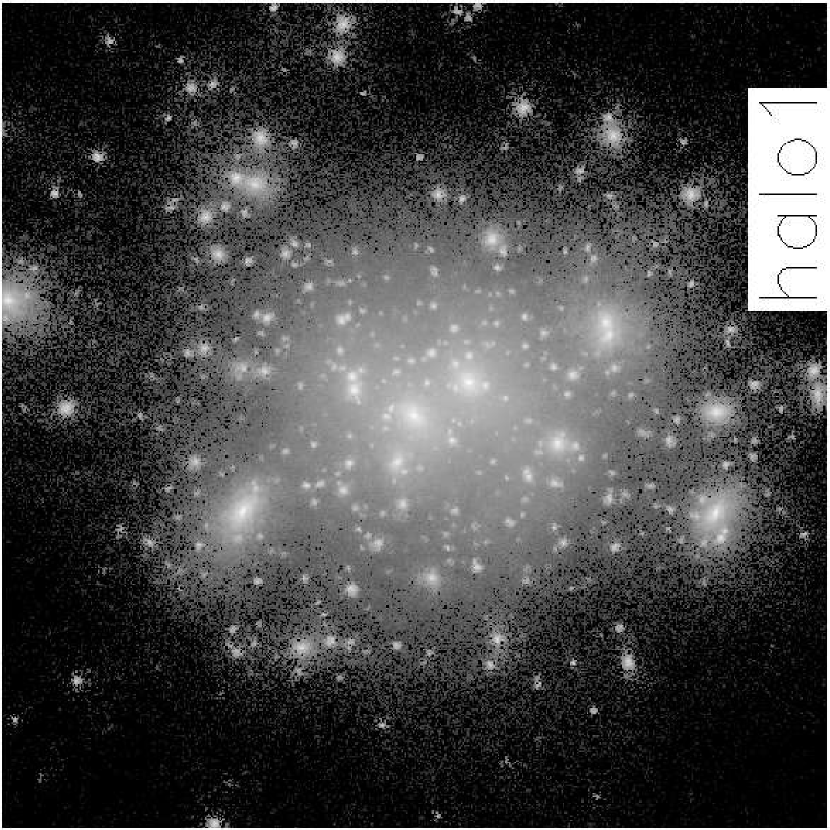
Figure 1: Dark matter distribution within the most massive halo in the LCDM100 simulation. The physical size of the figure is 2 times the halo virial radius.

The main simulation used in this paper is a $\rm P^{3}M$ cosmological simulation of $512^{3}$ particles in a box of $100\,h^{-1}{\rm{Mpc}}$. The underlying cosmological model is the standard concordance model with the density parameter $\Omega_{\rm m,0}=0.3$ , the cosmological constant $\Omega_{\Lambda,0}=0.7$ and the Hubble constant $h=0.7$ in units of $100\,{\rm{km\,s^{-1}}}{\rm Mpc}^{-1}$. The initial density field is assumed to be Gaussian with a Harrison-Zel’dovich primordial power spectrum and with an amplitude specified by $\sigma_{8}=0.9$, where $\sigma_{8}$ is the r.m.s. fluctuation of the linearly evolved density field in a sphere of radius $8\,h^{-1}{\rm{Mpc}}$. This simulation, which started at redshift $z_{i}=72$, is evolved by 5000 time steps to the present $z=0$ with our vectorized parallel $\rm P^{3}M$ code (Jing & Suto 2002) at the VPP5000 Fujitsu supercomputer of the National Astronomical Observatory of Japan. The force softening length $\eta_{f}$ (S2 type, Hockney & Eastwood 1981) is $10\,h^{-1}{\rm{kpc}}$ comoving, and the particle mass $m_{p}=6.2\times 10^{8}\,h^{-1}{\rm M_{\odot}}$. Because these simulation parameters are very similar to those adopted in many high-resolution re-simulations of individual cluster halos (Moore et al. 1999, Jing & Suto 2000, Fukushige & Makino 2001, 2003, Power et al. 2003, Diemand et al 2004), we have achieved a resolution that can resolve subhalos within massive halos. As we will see below, this is crucial for modeling correctly the mergers of galaxies in dark halos. The over-merging problem, which exists in many previous studies of structures of dark matter halos and semi-analytic models of galaxy formation based on cosmological $N$-body simulations, is greatly alleviated in our model. As an illustration, we show in Figure 1 the density distribution of dark matter particles within the largest dark halo in the simulation. As one can see, many subhalos remain intact during the evolution. We have estimated the mass function of the subhalo population (defined in §2.2), and found a good agreement with the subhalo mass functions obtained in previous halo re-simulations (e.g. SWTK) down to a mass of about $6.2\times 10^{10}\,h^{-1}{\rm M_{\odot}}$ (100 particles). This simulation was used to derive the triaxial model for dark matter halos in Jing & Suto (2002), to which we refer the reader for some complementary information about the simulation. We will call this simulation L100 in the following.

Although a box of $100\,h^{-1}{\rm{Mpc}}$ usually can be regarded as a typical volume in the universe, the most massive clusters with masses larger than $\sim 10^{15}\,h^{-1}{\rm M_{\odot}}$ may still be under-represented, because of the wavelength cutoff beyond the simulation box. Therefore, we have carried out simulations separately for 20 such massive halos with the nested-grid $\rm P^{3}M$ code of Jing & Suto (2000). These massive halos are picked up from a cosmological simulation of $256^{3}$ particles in a box of $300\,h^{-1}{\rm{Mpc}}$, and they are the most massive halos in the simulation. We do not impose any other criterion on the selection of these halos, and so the halo sample should be unbiased. In the re-simulations, each of the massive halos is represented by about $2\times 10^{6}$ particles within the virial radius, and so the particle mass is $(0.5\sim 1)\times 10^{9}\,h^{-1}{\rm M_{\odot}}$, comparable to the particle mass in L100. The force softening is also about $10\,h^{-1}{\rm{kpc}}$, but the simulations have been evolved by 20000 time steps (this choice of time steps was later found to be too conservative). This sample will be used to populate massive halos with galaxies in a set of simulations of $300\,h^{-1}{\rm{Mpc}}$ box in a subsequent paper. Here we only use the first halo $CL1$ to compare our results for cluster galaxies with observations and with those obtained by Springel et al. (2001). In addition to those simulations, we have also a cosmological simulation of $256^{3}$ particles in a box of $25\,h^{-1}{\rm{Mpc}}$, which has $\eta_{f}=5\,h^{-1}{\rm{kpc}}$ and is evolved with 5000 time steps. This simulation (referred to as L25 in the following) has a better mass resolution (8 times smaller in particle mass) than the L100 simulation. We will use this simulation to examine the mass resolution effect on the properties of galaxies at the faint luminosity end. All the three sets of simulations have the same model parameters. The L100 and CL simulations have 60 outputs from $z=15$ equally spaced in $\log_{10}(1+z)$, and the L25 has 165 outputs. These outputs are used to construct the merging trees of dark halos.

2.2 Merger trees of subhalos

The dark matter halos are identified in the simulations using the Friends-of-Friends method (FOF) with a linking length equal to 0.2 of the mean particle separation. The technique rarely breaks a physically bound halo into pieces; rather, it may combine two nearby distinct halos into one halo in some cases, if there is a thin bridge of particles between the two halos. Furthermore, in our high resolution simulations, galactic halos falling into a more massive halo (say, a cluster halo) can survive the tidal disruption of the massive halo for a considerable period of time. As emphasized in SWTK, it is important to follow the trajectories of these subhalos, not only because they can provide us with the position and velocity of the galaxies they host, but also because they allow us to accurately follow the merging histories of galaxies (as discussed in §1). We identify the subhalos within the FOF halos with the SUBFIND routine of SWTK, which kindly has been made available to us by Volker Springel.

The SUBFIND routine finds self-bound halos and subhalos in a single output of a simulation. Starting from a FOF halo, the SUBFIND first locates local overdense regions as subhalo candidates. For each particle in the input FOF halo, the local density is computed using the common SPH technique. The smoothing length is taken to be the distance to the $N_{\rm dens}$-th nearest neighbor particle, and the density is smoothed by a kernel interpolation of the $N_{\rm dens}$ particles. The particles are sorted in order of decreasing density, and are assigned to subhalo candidates sequentially. When the $i$-th particle with density $\rho_{\rm i}$ is considered, a set of particles $A_{i}$ is defined as the set of its $N_{\rm ngb}$ nearest neighbors. In the set of $A_{i}$ particles, we select a subset of particles with density higher than $\rho_{i}$ and among those a set $B_{i}$ is selected as the set of the two closest particles. Particle $i$ is assigned to a subhalo candidate according to the set of particles $B_{i}$. If there is no particle in $B_{i}$, particle $i$ is at the local maximum of the smoothed density field, and a new subhalo candidate is created around particle $i$. If there is only one particle $j$ in $B_{i}$, the particle $i$ is likely within the subhalo that contains particle $j$, and thus is assigned to that subhalo candidate. If there are two particles $j$ and $k$ in $B_{i}$, there are two possibilities. Either the two particles $j$ and $k$ are in two different subhalos. In this case, the particle $i$ is said to be a saddle point connecting these subhalos, and a new subhalo candidate is formed by joining these two subhalos with particle $i$. Or, as the second possibility, the two particles $j$ and $k$ are in the same subhalo. In this case, particle $i$ is simply added to this subhalo candidate. In this way, a set of subhalo candidates are created for the FOF group. Then the particles in each subhalo candidate are checked whether they are bound in the center-of-mass reference frame, and the particles that have positive total energy are removed iteratively until all the particles are bound. The bound subhalo candidates thus constructed establish a hierarchy of small subhalos in larger subhalos. The subhalos that have only one saddle point are at the highest level of the hierarchy, and those with more saddle points are at a lower level of hierarchy. In this case, one particle may be assigned more than once to subhalos at different levels of the hierarchy. SUBFIND keeps the identity of the particles only at the highest possible level of the hierarchy, thus producing a unique subhalo catalog. The algorithm can easily deal with the subhalo-within-subhalo problem, as well as the problem of the FOF algorithm that two halos with a thin bridge of particles are identified as one halo. With these subhalo catalogs at different outputs, we construct the merging trees for subhalos.

In Figure 2, we show the mass functions of the subhalos in the L100 simulation (upper panel) and in the cluster halo re-simulations (low panel). For the L100 simulation, the results are the average values for the host halos in the mass ranges indicated in the figure. For the cluster halo re-simulations, the mass functions are for individual halos. These mass functions are plotted down to a mass corresponding to 16 simulation particles. The mass functions for the most massive halos in the L100 simulation and for the individual cluster re-simulations agree well with each other over the whole mass range. For comparison we show the prediction of SWTK by the thick solid line. It was found that the mass function have a little steeper slope than that of SWTK and close to the reported relation $n\propto m_{\rm sub}^{-2}$ by Diemand et al (2004). The subhalo mass function for halos with masses $m_{\rm halo}=5\times 10^{13}\,h^{-1}{\rm M_{\odot}}$ has a similar slope to that of cluster halos, but the amplitude is a factor of about 2 lower. This decrease in amplitude with host halo mass is quantitatively in agreement with the recent results obtained by Gao et al. (2004) based on a cosmological simulation that has slightly lower resolution than our L100. The figure also shows that the subhalo mass function breaks away from the power law, $n\propto m_{\rm sub}^{-2}$, for subhalos containing less than about 20 simulation particles in the L100 simulation, indicating that the mass function may be affected by the resolution effect at such a mass scale. These results indicate that our L100 simulation can be used to probe subhalos that contain more than 50 simulation particles (i.e. with masses $\gtrsim 3\times 10^{10}\,h^{-1}{\rm M_{\odot}}$). For a subhalo with less than 50 particles, we use the L100 simulation to follow its merger history until it reaches the resolution limit, i.e. 10 particles. We do not use the Monte Carlo method to follow the merger histories of low mass halos, but instead we will use the L25 simulation (with a higher mass resolution) to check the resolution effect. As we will show in Section 4.1, the resolution limit has little effect on the predicted luminosity function for $M_{g}-5\log h<-17.5$, but it under-predicts the number count of faint galaxies ($-17.5<M_{g}-5\log h<-15.5$) by $\sim 30\%$.

3 The galaxy population

We implement the SAM in our $N$-body simulations following SWTK, but our model also includes the chemical evolutions of galaxies and the inter-galactic medium, as well as dust extinction effects on observational quantities, such as luminosity and color. Our model is therefore closer to the model adopted in a more recent publication from the same group (De Lucia et al. 2004), although there are differences in the choice of model parameters. For example, De Lucia et al. have chosen a high yield of metal production in order to match the observed high metallicity of the intracluster medium (ICM). Since the high metallicity leads to rapid gas cooling, they had to use a rather high feedback efficiency to suppress the formation of luminous galaxies. In our model, we adopt a metal yield and a feedback efficiency that are more moderate. For completeness, we briefly describe our SAM in this section. Since our main treatments about galaxy formation are similar to SWTK, we will compare in some detail our prescription and results with those in SWTK and related investigations (e.g. KCDW, De Lucia 2004).

3.1 Galaxy population in the subhalo scheme

In the subhalo scheme, there are three distinct populations of galaxies that are associated with FOF halos. The largest subhalo in a FOF halo is called the main halo, and the main halo always hosts a galaxy at its center, which we call the central galaxy. The central galaxy is assumed to have the same position and velocity as the most bound particle of the main halo. Any other subhalo in the FOF halo also hosts a galaxy at its center. These galaxies, called halo galaxies, were central galaxies before their host halos fell into a larger halo. They are assigned the positions and velocities of the most bound particles of their host subhalos. The halo galaxies have a physical status very similar to that of the central galaxies, except that the central galaxies are fed by gas cooling flows, while the halo galaxies are not. When two or more halos and/or subhalos merge, the smaller halo (subhalo) may be destroyed, thus losing its identity as a subhalo in the SUBFIND algorithm. A subhalo may also be tidally disrupted after passing through dense regions in the main halo. A galaxy that was a central or a halo galaxy at an earlier epoch, but whose host (sub)halos disappeared from the SUBFIND catalog at some later time, is attached to the most bound particle of its host (sub)halo at the time just before the (sub)halo is disrupted. Such galaxies are called satellite galaxies.

The transformation of galaxies from one population to another is governed by the subhalo merging trees constructed from the SUBFIND catalogs at different outputs of the simulation. Consider two successive outputs at redshifts $z_{a}$ and $z_{b}$ ($z_{a}<z_{b}$). The subhalo $S_{b}$ at redshift $z_{b}$ is said to be a progenitor of a subhalo $S_{a}$ at a later time $z_{a}$ if more than half of the $N_{\rm link}$ most-bound particles of $S_{b}$ are contained in $S_{a}$. As in SWTK, we take $N_{\rm link}$ to be 10. After excluding those volatile subhalos at $z_{b}$ that are not a progenitor to any subhalo or FOF group at the later time $z_{a}$, each subhalo at $z_{b}$ must be a progenitor to one and only one subhalo at $z_{a}$. A subhalo at $z_{a}$ may have more than one progenitor at $z_{b}$, and the most massive of them is referred to as the main progenitor. In the case that a subhalo at $z_{a}$ has no progenitor, the subhalo is usually the main halo of a FOF group newly formed between $z_{a}$ and $z_{b}$, and a central galaxy is created for the subhalo. For a subhalo at $z_{a}$ that has at least one progenitor, the central (halo) galaxy of its main progenitor at $z_{b}$ is updated to be its central (halo) galaxy, and all the other galaxies of the progenitor subhalos (including the satellites of the main progenitor) become the satellite galaxies of the subhalo at $z_{a}$. The satellite galaxies are assumed to merge later with the central (halo) galaxy of the subhalo– after a dynamical friction timescale (see §3.2.5 for details).

The evolution of galaxies is assumed to be driven by the physical processes to be described in detail in Section 3.2. We solve the differential equations governing galaxy evolution using a time step smaller than the time interval between two successive simulation outputs. Typically, 20 steps are used for each interval between two successive outputs.

In passing, we mention that the virial mass $m_{\rm vir}$ of the main halo is defined as the mass enclosed by the virial radius $R_{\rm vir}$, within which the mean density is $\Delta_{c}(z)$ times the critical density of the universe at the redshift $z$ in consideration. $\Delta_{c}(z)$ can be calculated analytically from the spherical collapse model (e.g. Kitayama & Suto 1996). Here we use the fitting formula provided by Bryan & Norman (1998),

$$\Delta_{c}(z)=18\pi^{2}+82x-39x^{2}\,,$$ (1)

where $x=\Omega(z)-1$, and $\Omega(z)$ is the density parameter at redshift $z$. For a subhalo, the virial mass is simply the total mass of all the particles in the subhalo, and the dynamical time $t_{\rm dyn}$ and virial velocity $V_{\rm vir}$ are kept at the values the subhalo had just before it merged into a bigger halo.

3.2 Physical Processes

In addition to the formation of the halo/subhalo population, galaxy formation and evolution also involve many other physical processes. In this paper, we attempt to take into account all processes that are known to be important for the formation and evolution of galaxies. These include: (1) radiative cooling of the hot gas within the main halo; (2) star formation in the cold gas, and energy feedback into the cold gas by supernova explosions; (3) chemical evolution in the cold and the hot gas, and in stars; (4) mergers of galaxies, star bursts, and the transformation of galaxy morphologies; (5) spectro-photometric evolution of individual galaxies; and (6) the effect of dust extinction on observational quantities.

3.2.1 Cooling of hot gas

As in White & Frenk (1991), the hot gas within a halo is assumed to be distributed in an isothermal sphere $\rho_{\rm g}(r)$ with a virial temperature $T=35.9(V_{\rm vir}/\,{\rm{km\,s^{-1}}})^{2}{\rm K}$. The local cooling time at a given radius $r$ is

$$t_{\rm cool}(r)=\frac{3}{2}\frac{kT\rho_{\rm g}(r)}{\overline{\mu}m_{\rm p}n_{\rm e}^{2}(r)\,\Lambda(T,Z)}\,,$$ (2)

where $\overline{\mu}m_{\rm p}$ is the mean particle mass, $n_{\rm e}(r)$ the number density of electron at $r$, and $\Lambda(T,Z)$ the cooling function, which depends both on the temperature $T$ and the metallicity $Z$ of the hot gas. We use the cooling functions tabulated in Sutherland & Dopita (1993). The chemical evolution of the hot gas is described in §3.2.4.

As in KCDW, we define the cooling radius $r_{\rm cool}(z)$ as the radius at which the cooling time $t_{\rm cool}$ is equal to the age of the universe $t_{\rm age}(z)$ at redshift $z$. If the cooling radius is smaller than the virial radius, the mass of gas cooled per unit time, i.e. the mass cooling rate, in the halo is approximated by

$$\dot{m}_{\rm cool}=4\pi\rho_{\rm g}(r_{\rm cool})r^{2}_{\rm cool}\dot{r}_{\rm cool}\,,$$ (3)

where a dot denotes the derivative with respect to time $t$. For the isothermal sphere distribution considered here, the cooling rate can be written as

$$\dot{m}_{\rm cool}=\frac{m_{\rm hot}}{R_{\rm vir}}\frac{r_{\rm cool}}{2t_{\rm cool}}\,,$$ (4)

where $m_{\rm hot}$ is the total hot gas in the halo. Note that this relation is derived under the assumption that the isothermal sphere is static. It implies that all the gas within the cooling radius can cool in a time interval that is twice the cooling time. In what follows we will assume this relation to hold during the evolution of a relatively massive halo, with $m_{\rm hot}$ being the total amount of hot gas at the time in consideration. For small halos or halos at high redshift, the cooling time can be smaller than the age of the universe even at the virial radius. In such halos, all the gas within the virial radius can cool, and so the mass cooling rate is limited by the rate at which gas is accreted into the system, rather than by radiative cooling. In this case, we write the mass ‘cooling’ rate as

$$\dot{m}_{\rm cool}=\frac{m_{\rm hot}}{t_{\rm cool}}\,,$$ (5)

where $t_{\rm cool}$ is to be specified below. Note that for halos where $r_{\rm cool}=R_{\rm vir}$, there is a jump of a factor of 2 between equation (4) and equation (5), which is entirely due to the simple prescription we adopt. In reality, the transition must be smooth, which can be made by joining equations (4) and (5) with a smooth function. This does not lead to any noticeable effects, and so we will ignore such details.

We assume a universal baryon fraction $f_{b}$ for every halo, and the hot gas available for cooling is:

$$m_{\rm hot}=f_{b}m_{\rm vir}-\sum_{i}[m_{\star}^{(i)}+m_{\rm cold}^{(i)}+m_{\rm eject}^{(i)}]$$ (6)

where $f_{b}=\Omega_{b}/\Omega_{0}$, and $m_{\rm\star}^{(i)}$, $m_{\rm cold}^{(i)}$, and $m_{\rm eject}^{(i)}$ are, respectively, the masses in stars, in cold gas, and ejected from stars. The sum is over all the galaxies in the halo in consideration. Because the ejected mass is assumed to be mixed into the hot gas in the current work, the term $m_{\rm eject}^{(i)}$ is set to be 0 in the above equation.

SWTK defined the cooling radius by equating $t_{\rm cool}(r)$ to the dynamical time of the halo, i.e., $t_{\rm cool}=t_{\rm dyn}=R_{\rm vir}/V_{\rm vir}$. On the other hand, KCDM used $t_{\rm cool}=t_{\rm age}$, i.e. equation (4) for large halos where $r_{\rm cool}<R_{\rm vir}$, while $t_{\rm cool}=t_{\rm dyn}$ for smaller halos (eq.5). Note that the cooling rate given by $t_{\rm cool}=t_{\rm dyn}$ is a factor of 2 to 4 higher than that given by $t_{\rm cool}=t_{\rm age}$, and so the two assumptions in general give quite different results for the galaxy population.

Unfortunately, there is no good physical reason to prefer either of the two assumptions. Although radiative cooling is a well-understood process, the gas cooling rate in a halo depends sensitively on the assumed density and temperature profiles of the gas. The assumption usually made in SAMs is that the gas is heated by gravitational collapse to a temperature close to the virial temperature of the dark halo and that the gas distribution in a dark halo is close to that of an isothermal gas in hydrostatic equilibrium in the halo potential. However the heating and cooling of gas in a dark halo are more complicated than this assumption implies. On the one hand, detailed analytical models and hydrodynamic simulations show that the halo gas in low-mass halos may never be heated to the virial temperature of the halo (e.g. Birnboim & Dekel 2003; Keres et al. 2004), and so the amount of cold gas may be underestimated by the above formulae. On the other hand, if gas in protogalactic halos is preheated to some finite entropy, the gas distribution around a small dark matter halo may be much more extended, and the rate of gas cooling in such systems can be significantly reduced (Mo & Mao 2002; Oh & Benson 2003). It has been shown by some SAMs that the suppression of gas cooling in small halos by photoionization heating may have significant impact on the faint-end slope of the galaxy luminosity function (e.g. Somerville 2002; Benson et al. 2002; Benson et al. 2003), but such models depend on the details of the implementation of the process. In this paper, instead of introducing such complicated physical models, we consider a simple model, in which $t_{\rm cool}$ is assumed to be equal to $t_{\rm age}(z)$. This assumption is consistent with the results of Brinchmann et al. (2004) who have shown that the local star-forming population of galaxies have roughly constant star formation rates over a time scale comparable to the present age of the Universe. As we will see below, this assumption leads to sufficient suppression of star formation in low-mass halos.

It has been pointed out by Kauffmann et al. (1993) that gas cooling (or star formation) must be strongly suppressed in the most massive halos so as not to produce too many super-luminous galaxies (see also Benson et al. 2003). As we will see below, the assumption about this suppression has significant impact on the prediction of the number of bright blue galaxies. As in Kauffmann et al. (1993), we consider a case in which gas cooling is simply switched off for halos with circular velocity larger than $390\,{\rm{km\,s^{-1}}}$. Since there is no solid physical motivation for this assumption, we will discuss another simple model for the shut-off of cooling in subsection 4.2.

3.2.2 Star formation

We model the star formation rate $\psi$ as :

$$\psi=\alpha m_{\rm cold}/t_{\rm d}\,.$$ (7)

In the above equation, $\alpha$ is the star formation efficiency, and $t_{\rm d}$ is the dynamical time of the galaxy (not the halo). As in SWTK we use $t_{\rm d}=0.1\times R_{\rm vir}/V_{\rm vir}$. Note that other choices, such as a constant $t_{\rm d}$, have also been used in the literature (Somerville & Primack 1999). For a satellite galaxy, we keep the dynamical time $t_{\rm d}$ to be equal to the value the galaxy had when it was last a central or halo galaxy. The star formation efficiency $\alpha$ is assumed to depend on the circular velocity of the galaxy (Cole et al. 1994; 2000). Following De Lucia et al. (2004), we take

$$\alpha=\alpha_{\rm 0}\left(\frac{V_{\rm vir}}{220\,{\rm{km\,s^{-1}}}}\right)^{n}\,,$$ (8)

where $\alpha_{0}$ and $n$ are treated as free parameters. Note that $\alpha$ cannot be larger than $1$. We take $\alpha=1$ if the above equation gives a value larger than 1. Note that $n=0$ gives a constant star formation efficiency, which is in fact consistent with the observations of high mass galaxies (e.g. Kennicutt 1998). On the other hand, there is evidence that low-mass galaxies convert cold gas into stars less efficiently than high-mass galaxies (e.g. Boissier et al. 2001, Kauffmann et al. 2003). In this case, $n$ should be positive. As shown by De Lucia et al. (2004), the assumed value of $n$ has significant impact on the predicted cold gas fraction and we note that $n$ also plays an important role in determining the metallicity and color of low-mass galaxies. In the present paper, we follow De Lucia et al. (2004) by setting $n=2.2$.

3.2.3 Feedback

For a given stellar initial mass function (IMF), the energy released by supernovae associated with massive stars is $\eta_{\rm SN}E_{\rm SN}$ for a unit solar mass of newly formed stars, where $E_{\rm SN}$ is $\sim 10^{51}{\rm erg}$, the typical kinetic energy of the ejecta from each supernova, and $\eta_{\rm SN}$ is an factor that depends on the form of the IMF. For the Scalo IMF (Scalo 1986), $\eta_{\rm SN}$ is about $5.0\times 10^{-3}$, and for the Salpeter (1955) IMF it is about $6.3\times 10^{-3}$ (Note that both cases are assumed to apply in the mass range $0.1M_{\odot}<m<125M_{\odot}$). The released energy is supposed to heat the cold gas and expel it from the cold gas disk. With an amount of $\Delta m_{\star}$ of newly formed stars, the amount of cold gas that can be heated can be expressed as,

$$\Delta m_{\rm eject}=\frac{4}{3}\epsilon\frac{\eta_{\rm SN}E_{\rm SN}}{V_{\rm vir}^{2}}\Delta m_{\star}\,,$$ (9)

where $\epsilon$ describes the feedback efficiency. We assume that the cold gas is reheated to the virial temperature of the subhalo in which the galaxy resides. There are at least two possibilities for the fates of the reheated gas. The first is that the reheated gas always stays in the halo and is added to the hot gas for later cooling. The SAM model based on this treatment of the reheated gas is usually called the retention model. Another possibility is that the reheated gas is ejected from the host halo. This ejected gas may be re-accreted by the halo after some time, say, one dynamical time of the halo. The SAM based on the this assumption is called the ejection model. It has been shown by SWTK that both the retention and the ejection models can be made to match most observations by adjusting model parameters, such as the star formation efficiency $\alpha$ and the feedback parameter $\epsilon$. In this paper, we only consider the retention model. Note that in both retention and ejection cases, there is the issue about the state of the heated gas when it is re-accreted. Usually, the re-heated gas is assumed to have completely forgot its thermal history when it is re-accreted. In reality, the heated gas may retain part of the entropy it gained and behave differently from the un-heated gas. Unfortunately, this process has not yet been implemented reliably in the current SAMs.

3.2.4 Chemical evolution

In the previous subsections, we have described the physical processes that govern the mass and metal exchange among the three main components, stars, cold gas, and hot gas, within a dark matter halo. Here we write down the equations describing these processes, so that we can follow the evolution of each individual component. We assume that a fraction $R$ of the mass in newly formed stars is recycled into the cold gas through stellar winds. For the Scalo IMF, $R\approx 0.4$, and for the Salpeter IMF, $R\approx 0.35$, according to the standard stellar population synthesis model (Cole et al. 2000). Thus, the change of the stellar mass in each galaxy is given by

$$\dot{m}_{\star}=(1-{\rm R})\psi\,.$$ (10)

The cold gas in a galaxy is increased by radiative cooling of the hot gas, and is reduced by the formation of new stars and by supernova feedback. Thus, the change in the cold gas in each galaxy is given by

$$\dot{m}_{\rm cold}=\dot{m}_{\rm cool}-(1-{\rm R})\psi-\dot{m}_{\rm eject}\,.$$ (11)

In our model, $\dot{m}_{\rm cool}=0$ for halo and satellite galaxies. In the retention model adopted in this paper, all the cold gas reheated by the galaxies is retained in the main halo, thus the change in the hot gas in the main halo is

$$\dot{m}_{\rm hot}=-\dot{m}_{\rm cool}+\sum_{i}\dot{m}_{\rm eject}^{(i)}\,,$$ (12)

where the summation is over all galaxies in the FOF halo. Now consider the metal contents in the three components. We assume a yield $p$ of metal for the conversion of a unit mass of cold gas into stars. All the metals produced are assumed to be returned to the cold gas instantaneously. Thus, the mass changes in heavy elements in the three components are respectively given by

$$\dot{m}_{\star}^{Z}=(1-R)Z_{\rm cold}\psi\,,$$ (13)

$$\dot{m}_{\rm cold}^{Z}=\dot{m}_{\rm cool}Z_{\rm hot}+p\psi-(1-R)Z_{\rm cold}\psi-\dot{m}_{eject}Z_{\rm cold}\,,$$ (14)

and

$$\dot{m}_{\rm hot}^{Z}=-\dot{m}_{\rm cool}Z_{\rm hot}+\sum_{i}\dot{m}_{\rm eject}^{(i)}Z_{\rm cold}^{(i)}\,,$$ (15)

where again the summation is over all the galaxies in the main halo, and $\dot{m}_{\rm cool}$ in Eq.(14) is set to be zero for all but the central galaxies. We have used the mean metallicities, $Z_{\rm cold}=m^{Z}_{\rm cold}/m_{\rm cold}$ and $Z_{\rm hot}=m^{Z}_{\rm hot}/m_{\rm hot}$ as the metallicities for the cold gas in a galaxy, and for the hot gas in a main halo, respectively. The ejected metals are assumed to have the same fate as the reheated gas.

When solving the above set of differential equations, we divide the time between two successive snapshots typically into 20 steps. As mentioned above, we keep the cooling rate $\dot{m}_{\rm cool}$ at a constant level between the two snapshots.

3.2.5 Halo mergers and galaxy mergers

With our high-resolution simulations, we are able to follow the formation, mass accretion, and mergers of (sub-)halos in detail. In our implementation of the SAM, we deal with these processes according to the (sub-)halo merger trees at each new snapshot of the simulation. For a newly formed halo of mass $m_{\rm vir}$, there is hot gas of mass $f_{b}m_{\rm vir}$ associated with it, and a new galaxy is being formed as the gas cools. The accreted mass is considered simply by updating the virial mass of the main halo (as well as other properties, such as the virial radius, circular velocity) and its hot gas in Eq. (6). When two or more (sub-)halos merge, the hot gas, if any, in the smaller halos, is added to that of the main halo that contains them. The galaxies in the smaller halos either become halo galaxies or satellite galaxies, depending on whether they are the central galaxies of the subhalos.

The merger of a halo galaxy with another halo galaxy or with the central galaxy is explicitly traced by our subhalo merger trees. For a satellite galaxy where a subhalo is absent in the simulation, we assume that it merges with its central or halo galaxy after a dynamical friction time scale $\tau$. We use the simple formula given in Binney & Tremaine (1987),

$$\tau=0.5\frac{f(\epsilon)V_{c}r_{c}^{2}}{CGm_{\rm sat}\ln\Lambda}\,,$$ (16)

to calculate $\tau$. As shown by Navarro et al. (1995), this formula provides a good fit to their numerical simulation studying the fate of a satellite $m_{\rm sat}$ orbiting in a halo of circular velocity $V_{c}$. In the above equation, $f(\epsilon)$ describes the dependence of $\tau$ on the orbit eccentricity $\epsilon$, and is approximated by $f(\epsilon)\sim\epsilon^{0.78}$ (Lacey & Cole 1993). As in previous SAMs, we adopt the average value $\langle f(\epsilon)\rangle\sim 0.5$ for $f(\epsilon)$ (e.g. Tormen 1997). $C$ in the above equation is a constant approximately equal to 0.43, and the Coulomb logarithm $\ln\Lambda$ is $\ln(1+m_{\rm vir}/m_{\rm sat})$. We take the satellite mass $m_{\rm sat}$ to be the virial mass of the galaxy when it was last a central or halo galaxy.

At each new snapshot of the simulations, the merger clock is set up for the new satellite galaxies in each subhalo, according to equation (16). For those satellites whose host subhalos do not change between two successive snapshots, the merger clocks are kept unchanged. In each time step $\Delta t$ in solving the equations (10)–(15), the merger clock time is reduced by $\Delta t$. A satellite galaxy is merged to its central or halo galaxy when its merger clock time becomes negative, and then is deleted from the galaxy list.

The physical properties of the merger remnant are modeled according to the mass ratio of the two galaxies that merge together. Here the mass of a galaxy is referred to its stellar component only. When the mass ratio of the smaller galaxy to the bigger one in a merger is less than 0.3, the merger is called a minor merger; otherwise, it is a major merger. In a minor merger, the cold gas of the smaller galaxy is put to the cold gas disk of the larger one, and its stellar mass is added to the bulge of the larger one. In a major merger, all the cold gas in the two galaxies is converted into stars instantly, and all the stellar mass in the disk and bulge components is transformed into a new bulge.

3.2.6 Photometric evolution of galaxies

We model the photometric evolution of galaxies using the stellar population synthesis (SPS) model of Bruzual & Charlot (1993). We use their recent SPS library (in 2000) that includes the metallicity effect on the photometric properties. The spectral energy distribution of a galaxy can be computed through

$$S_{\nu}=\int^{t}_{0}F_{\nu}(t-t^{\prime})\dot{m}_{\star}(t^{\prime})dt^{\prime}\,,$$ (17)

where $F_{\nu}$ is the spectral energy distribution for a single-age population of stars, which depends on the IMF, metallicity and age of the formed stars. The model of Bruzual & Charlot (1993) is used to produce tables for a single instantaneous burst of a unit stellar mass in which the metallicity changes from $0.0001$ to $0.1$. We interpolate the tables using a linear interpolation in $t$ and $\log(Z)$, and calculate the magnitudes for both the SDSS filters and the standard Johnson UBV filters.

As in Cole et al. (2000), we introduce a free parameter, $f_{visible}$, to take into account the fact that part of the newly formed stars may be invisible brown dwarfs ($m\leq 0.1M_{\odot}$). The mass fraction of the visible stars $f_{visible}$ is defined through

$$f_{visible}=\frac{\rm mass\,in\,visible\,stars}{(\rm mass\,in\,visible\,stars+mass\,in\,brown\,dwarfs)}$$ (18)

By definition, $f_{visible}$ cannot be larger than $1$. The inclusion of brown dwarfs makes the predicted luminosity smaller by a factor of $f_{visible}$. In this paper, we either assume $f_{visible}=1$, or when necessary tune the value of $f_{visible}$ to match the observed luminosity function in the SDSS $i$ band.

3.2.7 Dust extinction

The dust extinction model we use is similar to that of KCDW. We assume that the optical depth in the $B$-band scales with luminosity as

$$\tau_{\rm B}=\tau_{\rm B,\star}\left(\frac{L_{\rm B}}{L_{\rm B,\star}}\right)^{\beta}$$ (19)

with $\tau_{\rm B,\star}=0.8$, $L_{\rm B,\star}=1.3\times 10^{10}L_{\rm\odot}$ and $\beta=0.5$, as given by Wang & Heckman (1996). We use the model of Cardelli et al. (1989) to derive the ratio $\tau_{\lambda}/\tau_{\rm B}$. For a thin disk in which stars and dust grains have the same distribution, the total galactic extinction in magnitude is given by Tully & Fouqu$\acute{e}$ (1985):

$$A_{\lambda}=-2.5\log_{10}\left(\frac{1-e^{-\tau_{\lambda}\sec\theta}}{\tau_{\lambda}\sec\theta}\right)\,,$$ (20)

where $\theta$ is the inclination angle between the disk and the line of sight. In our model we assume that $\theta$ has a random distribution between $0$ and $90$. We apply the above equation only for the disk components, and we assume that there is no dust in the bulge component. As we will see, the inclusion of dust extinction improves the luminosity function in the bright end, especially for the blue band. Note, however, the dust extinction adopted here applies only to quiescent disk galaxies, but not to dust-enshrouded star burst galaxies. Thus, in our model, all star burst galaxies have very blue colors, although in reality they may be rather red due to dust extinction. In the present paper we do not include dust extinction for starburst galaxies, and we should keep this in mind when comparing model predictions with observations.

3.3 Model parameters and their impact on model predictions

Our SAM involves the following set of free parameters:

• IMF: the initial stellar mass function. In this paper, we adopt the Salpeter IMF for the major part of our discussion. We also consider the Scalo IMF as a comparison;

• $p$: the yield of metals from a unit mass of newly formed stars;

• $R$: the fraction of mass recycled into the cold gas by evolved stars;

• $\alpha_{\rm 0}$: the amplitude of the power-law star formation efficiency;

• $n$: the slope of the power-law star formation efficiency;

• $\epsilon$: the feedback efficiency;

• $f_{visible}$: the fraction of newly formed stellar mass that contributes to the luminosity of a galaxy.

Note that some of the above-listed free parameters are not independent of each other. For example, for a given IMF, the parameter $R$ is determined by stellar evolution theory. For the Scalo IMF, $R$ is about $0.4$, and for the Salpeter IMF, $R$ is about 0.35. We will use these values for $R$. The yield $p$ given by stellar evolution theory is between 0.01 and 0.02 for both the Scalo and the Salpeter IMFs, but the model prediction is still quite uncertain. In practice, we constrain $p$ using the color-magnitude relation (CMR) of cluster ellipticals, since the CMR is sensitive to the changes in the metallicity and the luminosities and colors of elliptical galaxies are less affected by dust.

To fix the other four parameters, we use the following two observational inputs: the SDSS galaxy luminosity function in the $i$-band, and the cold gas content of the Milky Way. The luminosity in the $i$-band is neither sensitive to the recent star formation rate nor to the dust extinction, and so can be used quite reliably as an indicator for the total stellar mass. Thus, both the star formation efficiency and the feedback efficiency are expected to have a significant impact on the $i$-band luminosity function and the cold gas content of the Milky Way. As in SWTK, we require the predicted cold gas in Milky Way type galaxies to be about 8$\times 10^{9}\,h^{-1}{\rm M_{\odot}}$. We will always assume $f_{visible}=1$ (i.e. the mass locked in brown dwarfs is negligible), unless a value of $f_{visible}$ less than 1 has to be introduced in order to match the observed $i$-band luminosity function (only in Fig.7).

We have adjusted the model parameters by trials and tests. We find that although the model predictions can be affected in complicated ways by changing model parameters, the parameter space allowed by the observations is actually quite limited. In Table 1, we list the parameters that best match the observational inputs. These values of parameters are in good agreement with those adopted in many earlier papers on SAMs (e.g. De Lucia et al. 2004). In what follows we compare model predictions and observational results based on various properties of the galaxy population.

4 Comparison with the galaxy population at low redshift

In this section, we compare our model predictions with observations about the galaxy population at $z\sim 0$. These observations include the multi-waveband luminosity functions of galaxies obtained from the SDSS and the 2dFGRS; the $I$-band Tully-Fisher relation; the CMR of elliptical galaxies in clusters and in the general field; the metallicity of galaxies as a function of luminosity or rotation velocity; and the cold gas fraction in galaxies of different luminosities; Note that some of the comparisons are not independent tests, because they are used to calibrate the model parameters. As we will show, there is general agreement between model and observation for various properties of the galaxy population. This is encouraging, because it indicates that the basic assumptions made in the model may be not far from reality. However, we also find significant discrepancies between model prediction and observation, suggesting that further improvement has to be made in the SAM.

4.1 The multi-waveband luminosity functions of galaxies

Blanton et al. (2003a) estimated the luminosity functions of galaxies for the SDSS survey in the five SDSS wavebands ($u$, $g$, $r$, $i$ and $z$). Since the median redshift of the galaxies in their sample is about 0.1, they made the $K$-correction and evolution correction to the reference frame at $z=0.1$, and shifted the bandpasses by a factor of 1.1. For comparison with these results, we shift the SDSS filters to the blue by a factor 1.1 when calculating the luminosities of individual galaxies. Following the SDSS convention, the corresponding wavebands are denoted by $u^{0.1}$ for the $u$-band, $g^{0.1}$ for the $g$-band, and so on. The upper panels and the lower left one of Fig.3 present the predicted luminosity functions in the $u^{0.1},g^{0.1},r^{0.1},i^{0.1}$ bands, with the solid histogram showing the result for the Salpeter IMF, and the dotted histogram showing that for the Scalo IMF. The thick solid lines show the Schechter function fits to the corresponding SDSS luminosity functions (Blanton et al. 2003a). Note that the agreement at the $z^{0.1}$-band is similar to that of $i^{0.1}$ band, and we have omitted the plot. We note that these Schechter function fits provide quite accurate description for the observational data, except at the brightest ends ($M_{\rm r}-5\log_{10}h\approx-22.5$), where they underestimate the observed number of galaxies. As one can see from the figure, the predicted luminosity functions match well the observed ones in the red bands. In the lower right panel of Fig.3, we show the predicted K-band luminosity function. The smooth solid curve in this panel shows the result of the Schechter function fit obtained by Kochanek et al. (2001) from the 2MASS. This result is similar to that obtained by Cole et al. (2001). As we can see, the reasonably good agreement between model prediction and observation also extends to the $K$-band, in which galaxy luminosity traces the stellar mass. Thus, the SAM considered here can successfully reproduce the observed stellar mass distribution in the Universe.

As a further test, we compare our model prediction with the observational result of Madgwick et al. (2002) for the 2dF galaxy luminosity function at the $b_{j}$ band at $z=0$ (see the lower middle panel of Fig.3). In our model, we estimate the $b_{j}$-band magnitude of a galaxy using the relation $b_{j}=B-0.28(B-V)$ (Blair & Gilmore 1982), where $B$ and $V$ are the rest-frame Vega magnitudes in the $B$- and $V$- wavebands. Since the observed 2dF luminosity function has a steeper faint-end slope than the SDSS luminosity function in the blue-band, it is better matched by the model prediction at the faint end than is the SDSS $g$-band luminosity function. From now on, our discussion about the galaxy luminosity function will be based on results for the $u^{0.1}$, $g^{0.1}$, $r^{0.1}$ and $i^{0.1}$ bands.

Compared with previous predictions of the field luminosity functions based on the SAMs (e.g., KCDW), our model gives a much better match to the observed luminosity functions. For example, KCDW significantly overpredicted the number of galaxies brighter than $L_{\star}$ and underestimates the number of fainter galaxies. Consequently, the luminosity functions predicted in KCDW are much flatter around $L_{\star}$ than the Schechter function. A similar discrepancy was also revealed for the galaxy luminosity function in rich clusters by SWTK, when a treatment of the galaxy-galaxy mergers similar to KCDW was adopted. They attributed the discrepancy to the assumption made in KCDW on the dynamical friction time scale for satellite galaxies. With the use of their resolved subhalos in clusters, SWTK found that the satellite galaxies brighter than $L_{\star}$ in a halo merge into the central galaxy at a rate much slower than that given by the dynamical friction time scale of equation (16) (used in KCDW). For the same reason, our model can reproduce well the observed field galaxy luminosity functions at the bright end, because subhalos hosting bright galaxies are well resolved in our $N$-body simulations. To demonstrate this, we have considered a model in which the merger time scales of satellite galaxies are estimated from equation (16) rather than using the subhalo scheme. As shown by Figure 4, the luminosity functions predicted by such a model are much flatter than the observational results and significantly over-predict the number of bright galaxies. Although the luminosity function at the bright end can be reduced by adjusting model parameters, for example by reducing the star formation efficiency, this will reduce the luminosity function at $L\lesssim L_{\star}$, making a large discrepancy at the intermediate luminosity. It is the shape of the luminosity function that cannot be easily adjusted to match the observations in this model.

In our subhalo scheme, we have used equation (16) to estimate the merger time for the satellites that are currently not associated with subhalos. It is therefore possible that the merger time here is also under-estimated. We have tested whether the uncertainties of the merger time in such galaxies can have a significant impact on our model predictions, by increasing or decreasing the merger time by a factor of 2. The results are shown in Fig.5. Little change was found in the model luminosity functions. The reason is that the merger time of satellites in these galaxies is relatively long, because of the small mass ratio between the satellite galaxy and the central galaxy, and so mergers are unimportant anyway. For the bright end, the change of the merger timescale has only a minor impact, because the mass of a satellite galaxy is in general quite small compared to the bright galaxies.

In Fig. 6, we compare the predicted cluster luminosity function with the composite luminosity function of rich clusters in the 2dFGRS by De Propris et al. (2003). Here we use one of our high-resolution cluster simulations, C1 (other clusters give similar results). Because the composite LF given by De Propris et al is not properly normalized for a given cluster mass, we adjust the amplitude of the observed LF to best match our model cluster LF and compare only the shape of the LF. The agreement is quite satisfactory. The absolute magnitude of the central galaxy in halo C1 is $M_{b_{j}}=-22.0$ in the subhalo scheme, compared with $M_{b_{j}}=-24.1$ in the case where galaxy mergers are not based on subhalos. The subhalo scheme also predicts more sub-$L_{\star}$ galaxies, in better agreement with the observation than the merger scheme solely based on the dynamical friction time scale. This result for the cluster LF is very similar to those obtained by SWTK and De Lucia et al. (2004), both using the subhalo scheme similar to the one used here. As in the previous works, our result demonstrates that resolving subhalos is an important ingredient to reproduce the exponential (Schechter) form at $L_{\star}$ of the composite cluster luminosity function.

As emphasized above, the main reason for the success of our model in reproducing the luminosity function of field galaxies is that we are able to follow the trajectories of massive galaxies using subhalos in our high-resolution simulations. This is an important result, because it implies that the shape of the observed galaxy luminosity function can be understood if galaxy mergers are modeled in a realistic manner. There is another factor, which also contributes to the success of our model, namely the cooling time scale we have adopted, $t_{\rm cool}=t_{\rm age}$ for all halos. If we followed SWTK in using $t_{\rm cool}=t_{\rm dyn}$, we would obtain a much higher amplitude for the luminosity function, because the cooling rate for massive halos at redshift $0$ is about a factor of $2.5$ higher. In this case, we have to multiply the luminosity of each galaxy by $f_{visible}=0.5$, i.e. to assume that about $50\%$ of the stellar mass is locked into brown dwarfs to best match the observed LF (see the dotted lines in Fig.7). This required $f_{visible}$ is too small to be realistic (Zhao et al. 1996, Somerville & Pirmack 1999). Also, with the assumption $t_{\rm cool}=t_{\rm dyn}$, the model predicts more galaxies at the fainter end, making faint-end slope of the luminosity function of cluster galaxies too steep.

As one can see, our model still predicts more faint galaxies (e.g. $M_{g}>-18.0+5\log_{10}h$ in the g-band) than are present in the SDSS observations. Detailed analysis of these over-predicted faint galaxies show that most of them are halo (satellite) galaxies in massive halos. Here we want to check whether the model prediction is significantly affected by numerical resolution. To do this, we applied the same SAM to the simulation L25, which has a mass resolution about ten times higher than L100. Fig.8 shows the results for the L25 simulation (dotted lines) in comparison to the results of L100 (solid lines). The resolution improvement does not seem to has any significant effect (at most $30\%$) on the predicted luminosity function at the faint end with $M_{g}>-17.5+5\log_{10}h$ . As we have shown above, the predicted faint end of the luminosity function is also insensitive to the assumed dynamical friction scale for satellite galaxies. The other factor we have examined is the feedback efficiency. We have considered a model assuming a feedback efficiency $\epsilon=0.2$ instead of $0.1$, and found that such a strong feedback can bring the number of faint galaxies into agreement with the observed LF, but the number density of galaxies with $L\sim L_{\star}$ is reduced too much to be compatible with the observation.

It is difficult to quantify how serious the faint end problem is. On the observational side, the faint-end slope of galaxy luminosity function is hard to determine, and there are considerable discrepancies among different sky surveys (LCRS, ESP, SDSS EDR, 2DF, SDSS DR1, etc. see Driver & De Propris 2003). Our model prediction is in good agreement with the steep faint-end slopes observed in the 2dF survey and in the ESP survey, but it is out of our scope to examine in which survey the faint galaxies are missed or/and misidentified.

Yang et al. (2003) have measured the mass-to-light ratio of dark halos in the $b_{J}$ band from the 2dFGRS using the halo model approach. They found that in terms of this ratio, galaxies are formed most efficiently in the halos of mass $m_{vir}=10^{12}h^{-1}{\rm M_{\odot}}$, and the galaxy formation is strongly suppressed both in lower and in higher mass halos. Such suppressions are expected in our semi-analytical model, because the hot gas cools less efficiently in cluster halos while the feedback effect can effectively heat up the cold gas and hence reduce the star formation in low-mass halos. It is interesting to see if our model prediction is in quantitative agreement with the measurement of Yang et al. (2003). This comparison is displayed in Figure 9. Except for $m_{vir}<10^{10}\,h^{-1}{\rm M_{\odot}}$, where the model prediction is limited by the simulation resolution and the observational measurement is limited by the small number statistics of galaxies, the agreement between the model and the observation is reasonable.

Based on the results obtained above for the $u$-band luminosity function, we see that our model predicts too many bright blue galaxies and insufficient number of blue galaxies with luminosities just below the characteristic luminosity. Our detailed analysis of the model prediction (with dust extinction) shows that at $z=0.1$ the brightest population in the $u$-band (with $M_{u}$ brighter than $-20.5+5\log h$) are dominated by starbursts that have just experienced a major merger. Most of the starbursts are in halos with mass around $10^{12}\,h^{-1}{\rm M_{\odot}}$. As we have mentioned before, the model prediction of the blue luminosities of these galaxies is quite uncertain, because our model does not include properly dust extinctions in dust-enshrouded starburst galaxies. The predicted excess of number of galaxies at lower luminosities ($M_{u}$ between $-20.5+5\log h$ and $-19+5\log h$) is mainly due to central galaxies in dark halos with masses around $10^{13}\,h^{-1}{\rm M_{\odot}}$ (see Fig.13). In our model, hot gas in such halos is allowed to cool continuously according to equation (3), although gas cooling is prohibited in more massive halos (see §3.2.1). The predicted excess of such blue galaxies is therefore due to the inadequate treatment of suppressing gas cooling in massive halos. It is possible to solve this problem by considering more realistic feedback processes in massive halos.

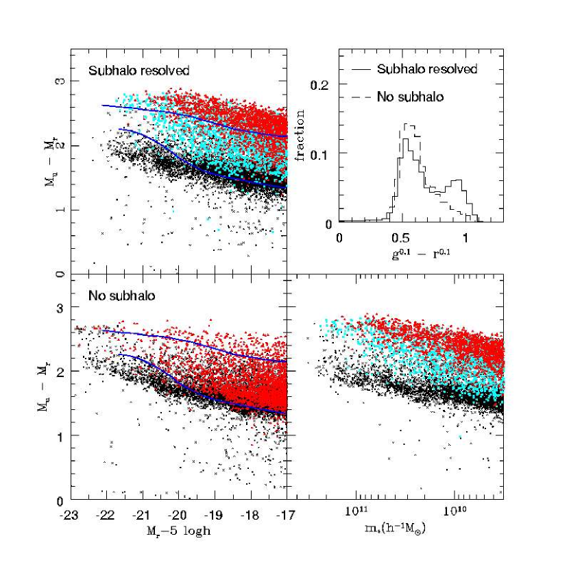
Figure 10: In the left panels: the color-magnitude diagram for all the galaxies in the L100 simulation at redshift $0$. The upper left left panel show results with subhalo resolved in the simulation and no subhalo resolved in lower panel. The upper right panel show the $g^{0.1}-r^{0.1}$ color distribution at $z=0.1$ and lower right show the color vs stellar mass of the model galaxies. In the plot crosses are central galaxies, squares are halo galaxies and triangles are satellites.

The cause of the deficit of blue galaxies with luminosities below $L_{*}$ is unclear (also present in Fig.10). One possibility is that the model assumes that the star formation rate in a quiescent disk is smooth with time, while in reality it may be intermittent, consisting of small bursts of star formation (Kauffmann et al. 2003). Such a change does not affect the total amount of stars that can form, and so does not change the luminosity functions in the red bands, but may produce more blue galaxies at the present time, as some of the low-mass systems may make excursions to the bursting phase at the present time. Another possibility is that the IMF is top-heavy, so that the fraction of UV-emitting massive stars is increased with respect to that of the Salpeter IMF. Clearly, further investigations along these lines are required to see if they are viable solutions to the problem.

4.2 Bimodal distribution in the color-magnitude diagram

As shown in Baldry et al. (2004a, 2004b), SDSS galaxies seem to exhibit a bimodal distribution in the color-magnitude diagram, in the sense that early-type and late-type galaxies show distinct colors for a given magnitude. To see if such a distribution can be reproduced in our model, we show in the upper left panel of Fig.10 the $M_{u}-M_{r}$ color as a function of $M_{r}$ for our model galaxies at redshift $0$. Central, halo and satellite galaxies are represented by black crosses, cyan squares and red triangles, respectively. The thick solid lines show respectively the fit results to the means of the Gaussian color distributions for the red and blue branches obtained by Baldry et al. (2004a). For comparison with the results of Blanton et al. (2003b), we also show in the upper right panel the $g^{0.1}-r^{0.1}$ color distribution at $z=0.1$ (the solid histogram), which is less dependent on dust extinction than the $u-r$ color. As in the observations, we see clearly two distinct branches in the case where subhalo scheme is used to follow the mergers of galaxies, with the blue branch more prominent than the red one. In the red branch, most galaxies are early-type galaxies . The mean $M_{u}-M_{r}$ color in this branch is around $2.3$ for faint galaxies ($M_{r}\sim-17+5\log h$), and becomes progressively redder for brighter galaxies. This prediction is very close to the observational result, although the predicted red branch has a larger dispersion and contains smaller number of very bright red galaxies. For the blue branch, the predicted mean $u-r$ color for galaxies fainter than $-20+5\log h$ is about $1.5$, slightly redder than the observational result ($u-r=1.3$). However, the model predicts too many bright galaxies in the blue branch. This problem is the same as one see in the $u$-band luminosity function shown in Fig. 3. The lower right panel shows the $u-r$ color versus stellar mass. The behavior seen here is similar to the color-magnitude relation.

It is instructive to examine what are the main factors that determine the predicted bimodal color distribution. We have made tests by changing the prescriptions of gas cooling, dust extinction and chemical enrichment. These changes can have some effects on the shape of the predicted color-magnitude relation, but do not change the bimodal behavior. On the other hand, if we use the old scheme instead of the subhalo scheme to describe the galaxy-galaxy mergers, the predicted bimodal feature is much weaker (see the lower left panel of Fig.10 and the dashed histogram in the upper right panel of the same figure). Note that in the upper left panel many of the bright galaxies in the red branch are halo galaxies, in which most of the cold gas has turned into stars and current star formation is at a low level, while in the old scheme no halo galaxies exist. The difference between the new and the old schemes can be understood as follows. In the subhalo scheme, galaxy mergers in a halo are allowed not only with the central galaxy, but also among halo and satellite galaxies. Since gas cooling is prohibited in halo and satellite galaxies, such mergers involve only evolved stellar population, producing new galaxies that are red. Consequently, many galaxies can stay red in the subhalo scheme. On the other hand, in the old prescription of galaxy-galaxy merging, galaxies in a halo merge relatively fast only with the central galaxy that may still have fresh cold gas. As a result, the number of red galaxies is reduced and the distinction between the red and blue populations is blurred. Thus, our ability to follow the evolution of subhalos seems to be the key in producing the observed bimodal color distribution.

Baldry et al. (2004a) show in their Figs.3 and 4 that most of the brightest galaxies are red, that the red branch becomes less prominent and the blue branch becomes more prominent as luminosity decreases. To compare our model prediction with their results, we show in Fig.12 the color distributions for galaxies in different luminosity bins. Overall, the predicted color distributions are similar to the observed ones, and in most cases the color distribution resembles the sum of double Gaussian. However, there is marked discrepancy between model and observation. At the high-luminosity end ($M_{r}-5\log h<-19.75$), the predicted colors in the blue branch are too blue, and the predicted red branch is too weak. We believe that this failure is related to our simplified treatment of the gas cooling in massive halos. As in many previous works (cf. Kauffmann et al. 1993), we cut off the gas cooling in very massive halos with the circular velocity above a given value ($390\,{\rm{km\,s^{-1}}}$ in our paper). Although there is strong observational evidence that the cooling should be suppressed in massive halos, there is no compelling reason why the gas cooling should be shut off according to the circular velocity. In fact, the number of the predicted most luminous red galaxies is very sensitive to this assumption. If we adopt a toy model in which we shut off the gas cooling according to the halo mass (instead of the circular velocity), we find that we can produce more brightest red galaxies and reduce the number of the brightest blue galaxies, while still keeping the luminosity function nearly unchanged (Kang et al. 2005). A more physical model is needed for suppressing the gas cooling in massive halos.

On the other hand, one also sees that for $M_{r}-5\log h>-18.75$, model galaxies in the blue branch have colors slightly redder than the observed galaxies. The observed blue colors imply that these galaxies have newly formed stellar population (Baldry et al. 2004b; Kauffmann et al. 2003). This may indicate that the treatment of star formation in our model is inadequate, and the starbursts triggered by minor mergers may also be an important missing ingredient for producing more blue galaxies.

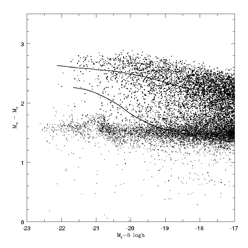
Figure 11: As in upper left panel of Fig.10 but without colors, and here the dust extinction is not included.

In our model that includes dust extinction, the predicted colors for galaxies with $M_{r}-5\log h<-20$ are still bluer than observed. The intrinsic colors of these galaxies are very blue, with $M_{u}-M_{r}\sim 1.6$, as shown in Fig.11. In order to see which type of galaxies contribute to the over-predicted blue galaxies, here we make an census of the galaxy population in the blue branch. In our model without dust, about $4\%$ percent of the very brightest galaxies with $M_{r}\simeq-23.25$ are recent star-burst galaxies in dark halos with virial mass around $10^{12}\,h^{-1}{\rm M_{\odot}}$. (these are ellipticals because they are associated with major mergers). Among the bright galaxies with $M_{r}<-20+5\log h$, about $10\%$ are E and S0 type galaxies according to the mass ratio of the merging progenitors and the fraction of star-burst galaxies is decreased to about $1\%$ percent. As we have discuss in §3.2.7 that we apply dust extinction correction to the galaxy with a prominent disk, so the ignore of dust reddening of star-burst galaxies is not reasonable for many observations show that dust correction should be important in those systems. The bright blue galaxies are still over-predicted even though the star-burst galaxies are extracted. This is for there are still cold gas available for new stars forming in the E, S0 and late type galaxies. We also found that the late type galaxies with bigger disks were also over-predicted compared with the morphology-classified K-band luminosity function of 2MASS (Kochanek et al. 2001). In order to see the origin of the problem, we examine where these blue bright galaxies are located. In Fig.13 we therefore plot the host halo mass for the blue ($M_{u}-M_{r}<2.0$) and red ($M_{u}-M_{r}>2.0$) galaxies in our L100 simulation. The main population of the blue bright galaxies are the central galaxies in halos of the velocity dispersion about $350\,{\rm{km\,s^{-1}}}$. In our model the gas cooling are still allowed in the halos and therefore the recent newly formed stars make their colors bluer. This is due to the inadequate treatment of cooling in massive halos, as discussed in the last subsection. Note that there is a feature in Fig.13, also in Fig.11. This is caused by the discontinuity of the gas cooling described by equation (4) and equation (5).

Baldry et al. (2004b) and Balogh et al. (2004) have shown that the color bimodality also depends on the environment defined by the local density of galaxies. The main properties of their observed color distribution can be summarized as follows: Firstly, for a given luminosity, the fraction of galaxies in the red sequence increases with local density. Secondly, faint galaxies are predominantly blue, except in very dense environments where a large fraction is also red. Finally, the most luminous galaxies are all red, independent of local environment. In our model, the first two properties are well reproduced. However, our model predicts a too strong blue branch in low and mediate density environments. The main reason for this discrepancy is that our model predicts too many luminous blue galaxies, because of the inadequate treatment of gas cooling in massive halos and because of the neglect of dust attenuation in massive starburst galaxies.

Since in the subhalo scheme halo- and satellite- galaxies can survive longer before merging with the central galaxies, our model predicts a large number of bright red galaxies at high redshift. In Fig.14, we show the distribution of galaxies with respect to the observed-frame $R-K$ color at $z=1$. Here only bright galaxies with M${}_{K}\leq-23.2$ were considered; the luminosity limit is chosen to match that of the Great Observations Origins Deep Survey (GOODS) sample used by Somerville et al. (2004) for our adopted cosmology. As shown by the solid histogram in Fig.14, about $10\%$ of our sample galaxies have $(R-K)_{AB}>3.5$. If we do not use the subhalo scheme to follow the galaxy-galaxy mergers, but use the conventional scheme based on dynamical friction, only $3\%$ of the bright galaxies have $(R-K)_{AB}>3.5$ (see the dotted histogram).

Based on multi-waveband photometries in deep fields and follow-up spectroscopic observations, such as the K20 Survey (Cimatti et al. 2002b), the GOODS (Giavalisco et al. 2004), and the Gemini Deep Deep Survey (GDDS, Abraham et al. 2004), it is now possible to identify a large number of bright galaxies at high redshifts. Such observations indicate that the number of bright red galaxies at $z\gtrsim 1$ may be larger than earlier predictions based on SAM (e.g. Cimatti et al. 2002a; Somerville et al. 2004; Glazebrook et al. 2004). Our results show that resolving subhalos may help alleviating this problem. We will make a detailed comparison of our model predictions with the observations at high redshift in a separate paper.

Before leaving from this subsection, let us consider the color-magnitude relation for the elliptical galaxies in clusters. In Fig.15, we present the predicted color-magnitude relation for the elliptical galaxies in the cluster simulation C1, and compare it with observation. We identify elliptical galaxies as the early-type galaxies with $M_{\rm bulge}-M_{\rm total}<0.8$ in the B band, and we show the predicted color-magnitude relation for individual model galaxies as solid triangles. The solid line shows the fit to the observation of Bower et al. (1992) for elliptical galaxies in the Coma cluster. As one can see, the observed trend is well reproduced in our model. The main reason for the color-magnitude relation in the model is the metallicity effect: more luminous galaxies have redder colors, because they have higher metallicity. This result is consistent with that obtained by De Lucia et al. (2004).

4.3 Tully-Fisher relation

In the upper panel of Fig.16, we plot the Tully-Fisher relation (hereafter TF relation) of the model Sb/Sc field galaxies against the observation of Giovanelli et al. (1997) at the I band:

$$M_{I}-5\log_{10}h=-21.00-7.68(\log_{10}W-2.5)\,.$$ (21)

The best fit of the observational result is shown as the solid line, while the dashed lines show the 1-$\sigma$ scatter. To select Sb/Sc galaxies from our SAM, we use the correlation between the $B$-band bulge-to-disk luminosity ratio and the Hubble-type given by Simien & de Vaucouleurs (1986). We select Sb/Sc galaxies according to the criterion, $1.2\leq M_{\rm bulge}-M_{\rm total}\leq 2.5$. We consider only the central galaxies with such Hubble types in the main halos. The velocity width $W$ is set to be 2 times the maximum circular velocity of the disk, and we have assume that the disk maximum circular velocity is $\sim 25\%$ larger than the circular velocity of the halo at its virial radius. This boost of disk maximum circular velocity is expected in a galaxy halo with typical concentration $c\sim 12$ assuming disk mass is negligible (e.g. Mo, Mao & White 1998). The triangles in Fig.16 are the results for our model Sb/Sc galaxies defined in this way. The figure shows that the scatter predicted by the model is significantly smaller than in the observational result. Note that in our modeling we have not taken into account the scatter in the relation between the line width and the circular velocity, neither have we included the observational errors in photometry and errors due to dust correction. Both can produce scatter in the TF relation. Overall, the predicted TF slope agrees quite well with the observed one, but the predicted luminosity for a given disk maximum circular velocity is lower than observed. Note that if dark halo responds to disk growth adiabatically, then the boost in the disk maximum circular velocity is expected to be larger than what is assumed above, making the discrepancy between model prediction and observation even large. This problem with the Tully-Fisher relation in the current $\Lambda$CDM model has been known earlier and is due to the fact that galaxy halos predicted by this model are too concentrated (e.g. Mo & Mao 2000 and references therein). One possible solution to this problem is that some dynamical processes during the formation of galaxies in dark halos can flatten dark matter halos (e.g. Mo & Mao 2004), so that the boost in the disk maximum circular is reduced. Indeed, if the boost is about 10%, then the predicted Tully-Fisher amplitude can match the observation.

4.4 Metallicity and cold gas fraction in spiral galaxy

Garnett (2002) studied the correlation between the metallicity of the interstellar gas in a galaxy with the luminosity and rotation velocity of the galaxy, for a sample of spiral and irregular galaxies. In Fig.17, we compare our model predictions with his results. We select a sample of galaxies from our SAM with $M_{\rm bulge}-M_{\rm total}>1$, corresponding to spiral and irregular galaxies according to our definition. The metallicity of the interstellar gas is obtained using the chemical evolution model described in §3.2.4. The figure shows that the observed correlation is well reproduced by our model. The vertical dashed line in the lower panel shows the rotation velocity at which the slope of the metallicity-rotation velocity relation changes significantly, as pointed out by Garnett.

In Fig.18, we show the cold gas fraction as a function of galaxy luminosity. Here again we compare our model prediction with the observational results of Garnett (2002). We define the cold gas fraction as $m_{\rm cold}/(m_{\rm cold}+m_{\star})$. As one can see, the predicted cold gas fraction is larger in fainter galaxies, which is consistent with the observed trend, and with the theoretical results obtained by Boissier et al. (2001) and Kauffmann et al. (2003). In our model, the predicted cold gas depends sensitively on the parameter $n$ in equation (8). Note that $n=0$ gives a constant gas fraction for all the spiral galaxies, a result obviously in conflict with the observation. A positive $n$ means that smaller galaxies have a lower star formation rate, which also leads to the metallicity trends shown in Fig.17.

5 Discussion and Conclusions

In this paper, we have modeled galaxy formation in a series of high-resolution $N$-body simulations of the standard $\Lambda$CDM model using the semi-analytical approach. One unique aspect of our analysis is that our model uses subhalos resolved in the $N$-body simulations to follow the mergers of galaxies in dark halos. The semi-analytical model we adopted for galaxy formation in dark matter halos is similar to those used in recent semi-analytical studies. We found that, if galaxy-galaxy mergers are followed by the merger histories of subhalos, rather than based on dynamical friction time scales, the semi-analytical model can match well the luminosity functions of galaxies in the bright end in various wavebands redder than the u-band. Our model also reproduces the main properties of the observed bimodal color distribution better than that model that do not resolve subhalos, although it still predicts too many bright blue galaxies. Resolving subhalos also produces many more bright red galaxies at high $z$, in better agreement with the observations. Once the model parameters are calibrated, the model can also match the observed metallicity-luminosity relation and metallicity-rotation velocity relation of spiral galaxies, the gas fraction in present-day spiral galaxies, and the color-magnitude relation for elliptical galaxies in clusters.

Overall, the model is very successful in explaining a wide variety of observational facts. This is encouraging, because it means that our understanding of galaxy formation in the standard $\Lambda$CDM model is on the right track. However, there are several important issues that remain unresolved. The first is the process that can effectively suppress star formation in low-mass halos. In this paper, instead of assuming an unrealistically high feedback efficiency, we have considered a model in which the gas cooling time in a dark halo is comparable to the age of the system. With such an assumption the faint-end slope of the luminosity function can be moderated. Although this assumption leads to predictions that can match the observational results better, and a prolonged cooling is expected if the intergalactic medium is preheated (Mo & Mao 2002, 2004; Oh & Benson 2003), the details of this process are still unclear. The second is concerned with the large number of bright blue galaxies predicted by the model. To address this issue in detail, we need a realistic dust model for starburst galaxies, as well as a realistic model for the gas cooling in massive halos. The third problem is that the current model predicts insufficient number of blue galaxies with intermediate luminosities, which indicates that either the IMF in disk galaxies is top-heavier than the Salpether IMF, or star formation in disk galaxies is intermittent. Finally, like many earlier analyses based on SAM, we found that the predicted Tully-Fisher zero point is too low, unless there are some processes that can significantly flatten CDM halos. Clearly, further investigations about the possible solutions are required in order to resolve these issues.

Table 1: Model parameters in our model

IMF	p	R	$\alpha_{0}$	$\epsilon$	$n$
Scalo	0.04	0.4	0.10	0.20	2.2
Salpeter	0.032	0.35	0.10	0.10	2.2

Figure 2: The mass function of subhalos as a function of the mass ratio of the subhalo to the host halo. The upper panel shows the mean result measured from the L100 simulation for three mass ranges of host halos (as indicated in the panel). The lower panel shows the results for the first three clusters in the sample of individual halo re-simulations. All the results are shown down to a subhalo mass corresponding to 16 simulation particles. For comparison, the mass function of cluster halos obtained by SWTK from their halo re-simulations is plotted as the solid line.

Figure 3: The multi-waveband luminosity function. The upper and the lower left panels show the SDSS luminosity functions in the $u^{0.1}$, $g^{0.1}$, $r^{0.1}$, and $i^{0.1}$ bands, respectively. The lower middle panel shows the result of the $b_{j}$-band luminosity function obtained from 2dFGRS, and the lower right panel shows the 2MASS $K$-band luminosity function. The smooth solid in each panel line show the Schechter function fit to the corresponding observational result (see text for references). In all the panels the histograms show our model predictions based on L100 assuming both the Salpeter IMF (solid) and the Scalo IMF (dotted).

Figure 4: The same as Fig.(3), but here subhalo scheme is not implemented. Here we plot the results using the Salpeter IMF.

Figure 5: The thick solid lines and the solid histograms are the same as in Fig.3. The dotted histograms result from decreasing (16) by half, and the dashed lines are from increasing the merger time by a factor of 2.

Figure 6: The luminosity function of cluster galaxies at the $b_{j}$-band. The data points connected by a solid line show the composite luminosity function given by De Propris et al. (2003).

Figure 7: The cooling time effect on the luminosity function. The solid lines are the same as in Fig1, and the dotted lines are for $t_{\rm cool}=t_{\rm dyn}$. Note that $f_{visible}$ is $0.5$ for $t_{\rm cool}=t_{\rm dyn}$.

Figure 8: Here we compare the effect of the simulation box on the predicted luminosity function for the models L100 and L25.

Figure 9: The ratio of the halo mass to the total luminosity $L_{b_{J}}$ of the halo in our semi-analytical model(the L100 simulation; the dashed line). For the comparison we also show this function determined from the 2dFGRS by Yang et al. (2003) using the halo model approach (the solid line).

Figure 12: The color distributions in absolute magnitude bins of 0.5. In each panel, the label magnitude is the median magnitude.

Figure 13: The host halo mass $m_{\rm vir}$ for galaxies of magnitude $M_{r}$ for blue and red galaxies in the L100 simulation.

Figure 14: The distribution of $(R-K)$ color for bright galaxies with $M_{K}\leq-23.2$ at $z=1$. The $(R-K)$ color in the Vega magnitude system was converted into the AB magnitude system using $(R-K)_{AB}=(R-K)_{Vega}-1.65$. The solid histogram shows the prediction in which subhalo scheme is used to follow the mergers among galaxies, while the dotted histogram shows the prediction in which mergers of galaxies are based on the dynamical friction formula.

Figure 15: Color-magnitude relation for early type galaxies in the C1 cluster simulation. The solid line shows the best fit to the observation of Coma cluster ellipticals by Bower et al. (1992)

Figure 16: The I band Tully-Fisher relation for spiral galaxies in the simulation L100.

Figure 17: The metallicity of the cold gas as a function of the luminosity in the B-band (the upper panel) or of the rotation velocity (the lower panel). The dots are from our SAM, and the squares are from the observations of Garnett (2002). The dashed line show the velocity where the metallicity-v_rot relation change significantly (Garnett).

Figure 18: The cold gas fraction as a function of the B-band luminosity. The triangles are from our SAM, and the squares are from the observations of Garnett (2002).

References

- Abel et al. (1997) Abel, T., Anninos, P, Zhang, Y., Norman, M., 1997, NewA, 2, 181
- (2) Abraham, R. G., et al., 2004, AJ, 127, 2455
- Baldry (2004) Baldry, I. K., Glazebrook, K., Brinkmann, J., Ivezic, Z., Lupton, R. H., Nichol, R., C., Szalay, A. S., 2004a, ApJ, 600, 681
- Baldry et al. (2004) Baldry, I. K., Balogh, M. L., Bower, R., Glazebrook, K., Nichol, R. C., 2004b, AIP Conf.Proc. 743, 106
- Balogh et al. (2004) Balogh, M. L., Baldry, I. K., Nichol, R. C., Miller, C., Bower, R., Glazebrook, K., 2004, ApJ, 615L, 101
- Baugh et al. (2004) Baugh, C. M., Lacey, C. G., Frenk, C. S., Granato, G. L., Silva, L., Bressan, A., Benson, A. J., Cole, S., 2004, MNRAS in press
- Benson et al. (2000) Benson, A. J., Cole, S., Frenk, C. S., Baugh, C. M., Lacey, C. G., 2000, MNRAS, 316, 107
- Benson et al. (2002) Benson, A. J., Lacey, C. G., Baugh, C. M., Cole, S., Frenk, C. S., 2002, MNRAS, 333, 156
- Benson et al. (2003) Benson, A. J., Bower, R. G., Frenk, C. S., Lacey, C. G., Baugh, C. M., Cole, S., 2003, ApJ, 599, 38
- Berlind & Weinberg (2002) Berlind, A. A., Weinberg, D. H., 2002, ApJ, 575, 587
- Berlind et al. (2003) Berlind, A. A., Weinberg, D. H., Benson, A. J., Baugh, C. M., Cole, S., et al., 2003, ApJ, 593, 1
- Binney & Tremaine (1987) Binney, J., Tremaine, S., 1987, ”Galactic Dynamics”, Princeton University Press, Princeton
- Birnboim & Dekel (2003) Birnboim, Y., Dekel, A., 2003, MNRAS, 345, 349
- Blair & Gilmore (1982) Blair, M., Gilmore, G., 1982, PASP, 94, 742
- (15) Blanton et al. 2003a, ApJ, 592, 819
- (16) Blanton et al. 2003b, ApJ, 594, 186
- Boissier et al. (2001) Boissier, S., Boselli, A., Prantzos, N., Gavazzi, G., 2001, MNRAS, 321, 733
- Bond et al. (1991) Bond, J. R., Kaiser, N., Cole, S., Efstathiou, G., 1991, ApJ, 379, 440
- Borys et al. (2003) Borys, C., Chapman, S. C., Halpern, M., Scott, D., 2003, MNRAS, 344, 385
- Bower et al. (1992) Bower, R. G., Lucey, J. R., Ellis, R. S., 1992, MNRAS, 589, 600
- Brinchmann et al. (2004) Brinchmann, J., Charlot, S., Kauffmann, G., White, S., Tremonti, C., Heckman, T. Brinkmann, J., 2004, MNRAS, 351, 1151
- Bruzual & Charlot (1993) Bruzual, A. G., Charlot, S., 1993, ApJ, 405, 538
- Bryan et al. (1994) Bryan, G. L., Cen, R. Y., Norman, M. L., Ostriker, J. P., Stone, J. M., 1994, ApJ, 428, 405
- Bryan & Norman (1998) Bryan, G. L., Norman, M. L., 1998, ApJ, 495, 80
- Bullock et al. (2002) Bullock, J. S., Wechsler, R. H., Somerville, R. S., 2002, MNRAS, 329, 246
- Calura et al. (2004) Calura, F., Matteucci, F., Menci, N., 2004, MNRAS, 353, 500
- Cardelli et al. (1989) Cardelli, J. A., Clayton, G. C., Mathis, J. S., 1989, ApJ, 345, 245
- Cen & Ostriker, (1993) Cen, R., Ostriker, J. P., 1993, ApJ, 417, 415
- Chapman et al. (2002) Chapman, S. C., Scott D., Borys, C., Fahlman, G. G., 2002, MNRAS, 330, 92
- (30) Cimatti, A., et al., 2002a, A&A, 391, 1
- Cimatti et al. (2002) Cimatti, A., et al., 2002b, A&A, 392, 395
- Coil et al. (2004) Coil, A. L. et al., 2004, ApJ, 609, 525
- Cole, (1991) Cole, S., 1991, ApJ, 367, 45
- Cole et al. (1994) Cole, S., Aragn-Salamanca, A., Frenk, C. S., Navarro, J. F., Zepf, S. E., 1994, MNRAS, 271, 781
- Cole et al. (2000) Cole, S., Lacey, C. G., Baugh, C. M., Frenk, C. S., 2000, MNRAS, 319, 168
- Cole et al. (2001) Cole, S., et al., 2001, MNRAS, 326, 255
- Colless et al., (2001) Colless, M., et al., 2001, MNRAS, 328, 1039
- Cooray & Sheth (2002) Cooray, A., Sheth, R., 2002, PhR, 372, 1C
- Couchman et al. (1995) Couchman, H. M. P., Thomas, P. A., Pearce, F. R., 1995, ApJ, 452, 797
- Cowie et al. (2002) Cowie, L. L., Barger, A. J., Kneib, J.-P., 2002, AJ, 123, 2197
- De Lucia et al. (2003) De Lucia G., Kauffmann, G., Springel, V., White, S. D. M., 2004, MNRAS, 349, 1101
- De Propris (2003) De Propris et al., 2003, MNRAS, 342, 725
- Diaferio (1999) Diaferio, A., Kauffmann, G., Colberg, J. M., White, S. D. M., 1999, MNRAS, 307, 537
- Diemand et al. (2004) Diemand, J., Moore, B., Stadel, J., 2004, MNRAS, 352, 535
- Driver & De Propris (2003) Driver, S. P., De Propris, R., 2003, ApSS, 285, 175
- Dusan et al. (2004) Keres, D., Katz, N., Weinberg, D. H., Dave, R., 2004, preprint (astro-ph/0407095)
- Efstathiou (1992) Efstathiou, G., 1992, MNRAS, 256, 43
- Eke et al. (1998) Eke, V. R., Navarro, J. F., Frenk, C. S., 1998, ApJ, 503, 569
- Fukushige et al. (2001) Fukushige, T, Makino, J., 2001, ApJ, 557, 533
- Fukushige et al. (2003) Fukushige, T, Makino, J., 2003, ApJ, 588, 674
- Gao et al. (2004) Gao, L., White, S. D. M., Jenkins, A., Stoehr, F., Springel, V., 2004, 355, 819
- Garnett (2002) Garnett, D. R., 2002, ApJ, 581, 1019
- Ghigna et al. (1998) Ghigna, S., Moore, B., Governato, F., Lake, G., Quinn, T., Stadel, J., 1998, MNRAS, 300, 146
- Giavalisco et al. (2004) Giavalisco, M., et al., 2004, ApJ, 600L, 93
- Giovanlli et al. (1997) Giovanelli, R., Haynes, M. P., Da Costa L. N., Freudling, W., Salzer, J. J., Wegner, G., 1997, ApJ, 477, 1
- Glazebrook et al. (1999) Glazebrook, K., Blake, C., Economou, F., Likky, S., Colless, M., 1999, MNRAS, 306, 843
- Glazebrook et al. (2004) Glazebrook, K., et al., 2004, Nature, 430, 181
- Hatton et al. (2003) Hatton, S., Devriendt, J., Ninin, S., et al. 2003, MNRAS, 343, 75
- Helly et al. (2003) Helly, J. C., Cole, S., Frenk, C. S., Baugh, C. M., Benson, A., Lacey, C., 2003, MNRAS, 338, 903
- Hockney & Eastwood (1981) Hockney, R. W., Eastwood, J. W., 1981, Computer Simulation Using Particles (McGraw Hill New York)
- Hughes et al. (1998) Hughes, D. H., et al., 1998, Nature, 394, 241
- Jing et al. (1995) Jing, Y. P., Mo, H. J., Börner, G., Fang, L. Z. 1995, MNRAS, 276, 417
- Jing et al. (1998) Jing, Y. P., Mo, H. J., Börner, G., 1998, ApJ, 494, 1
- Jing & Suto (2000) Jing, Y. P., Suto, Y., 2000, ApJ, 529, 69
- Jing & Suto (2002) Jing, Y. P., Suto, Y., 2002, ApJ, 574, 538
- Kang et al. (2005) Kang, X., Jing, Y. P., Mo, H. J., Börner, G., 2005, in preparation
- Katz & Gunn, (1991) Katz, N., Gunn, J. E., 1991, ApJ, 377, 365
- Kauffmann et al. (1993) Kauffmann, G., White, S. D. M., Guiderdoni, B., 1993, MNRAS, 264, 201
- Kauffmann & Charlot (1998) Kauffmann, G., Charlot, S. 1998, MNRAS, 294, 705
- (70) Kauffmann, G., Colberg, J. M., Diaferio, A., White, S. D. M., 1999a, MNRAS, 303, 188 (KCDW)
- (71) Kauffmann, G., Colberg, J. M., Diaferio, A., White, S. D. M., 1999b, MNRAS, 307, 529
- Kauffmann et al. (2002) Kauffmann, G., Heckman, T. M., White, S. D. M., Charlot, S., Tremonti, C., Peng, E. W., Seibert, M., Brinkmann, J., Nichol, R. C., SubbaRao, M., York, D., 2003, MNRAS, 341, 54
- Kennicutt (1998) Kennicutt, R. C., 1998, ApJ, 498, 541
- Keres et al. (2004) Keres, D., Katz, N., Weinberg, D. H., Dave, R., 2004, preprint, astro-ph/0407095
- Kitayama & Suto (1996) Kitayama, T., Suto, Y., 1996, ApJ, 469, 480
- Klypin et al. (1999) Klypin, A. A., Gottöber S., Kravtsov, A. V., Khokhlov, A. M., 1999, ApJ, 516, 530
- Kochanek et al. (2001) Kochanek, C. S., Pahre, M. A., Falco, E. E., Huchra, J. P., Mader, J., Jarrett, T. H., Chester, T., Cutri, R., Schneider, S. E., 2001, ApJ, 560, 566
- Kravtsov et al. (2004) Kravtsov, A. V., Berlind, A. A., Wechsler, R. H., Klypin, A. A., Gottloeber, S., Allgood, B., Primack, J. R., 2004, ApJ, 609, 35
- Lacey & Silk, (1991) Lacey, C., Silk, J., 1991, ApJ, 381, 14
- Lacey & cole (1993) Lacey, C. G., Cole, S., 1993, MNRAS, 262, 627
- Madgwick et al. (2002) Madgwick et al. 2002, MNRAS, 333, 133
- Maller et al. (2004) Maller, A. H., McIntosh, D. H., Katz, N., Weinberg, M. D., 2004, preprint, astro-ph/0304005
- Mathis et al. (2002) Mathis, H., Lemson, G., Springel, V., Kauffmann, G., White, S. D. M., Eldar, A., Dekel, A., 2002, MNRAS, 333, 739
- Menci et al. (2002) Menci, N., Cavaliere, A., Fontana, A., Giallongo, E., Poli, F., 2002, ApJ, 575, 18
- Mo et al. (1998) Mo, H. J., Mao, S., White, S. D. M., 1998, MNRAS, 295, 319
- Mo & Mao (2000) Mo, H. J., Mao, S., 2000, MNRAS, 318, 163
- Mo & Mao (2002) Mo, H. J., Mao, S., 2002, MNRAS, 333, 768
- Mo & Mao (2004) Mo, H. J., Mao, S., 2004, MNRAS, 353, 829
- Moore et al. (1999) Moore, B., Ghigna, S., Governato, F., Lake, G., Quinn, T., Stadel, J., Tozzi, P., 1999, ApJ, 524, 19
- Nagashima et al. (2002) Nagashima, M., Yoshii, Y., Totani, T., Gouda, N., 2002, ApJ, 578, 675
- Nakamura et al. (2003) Nakamura, O., Fukugita, M., Brinkmann, J., Schneider, D. P., 2003, preprint, astro-ph/0312519
- Navarro & White, (1994) Navarro, J., White, S. D. M., 1994, MNRAS, 267, 401
- Navarro et al. (1995) Navarro, J. F., Frenk, C. S., White, S. D. M., 1995, MNRAS, 275, 56
- Oh & Benson (2003) Oh, S. P., Benson, A., 2003, MNRAS, 342, 664
- (95) Peacock, J. A., Smith, R. E., 2000, MNRAS, 318, 1144
- Peacock et al. (2001) Peacock, J. A., et al., 2001, Nature, 410, 169
- Power et al. (2003) Power, C, Navarro, J. F., Jenkins, A., Frenk, C. S., White, S. D. M., Springel, V., Stadel, J., Quinn, T., 2003, MNRAS, 338, 14
- Pozzetti et al. (2003) Pozzetti, L., et al., 2003, A&A, 402, 837
- Press & Schechter (1974) Press, W. H., Schechter, P., 1974, ApJ, 187, 425
- Salpter (1955) Salpeter, E. E., 1955, ApJ, 121, 161
- Scalo (1986) Scalo, J. M., 1986, Fundamentals of Cosmic Physics, 11, 1
- Schneider (1999) Schneider, P., Ehlers, J., Falco, E. E., 1999, Gravitational lenses, A&A Library. Springer Verlag: Berlin
- Seljak (2001) Seljak, U., 2001, MNRAS, 325, 1359
- Simien (1986) Simien, F., Vaucouleurs, G., 1986, ApJ, 302, 564
- Skrutskie (1997) Skrutskie M.F., et al., 1997, in The Impact of Large-Scale Near-IR Surveys, eds. F. Garzon et al. Kluwer Academic Publishing Company Dordrecht, 1997, p25
- Smail et al. (2002) Smail, I., Ivison, R. J., Blain, A. W., Kneib, J.-P., 2002, MNRAS, 331, 495
- Somerville & Primack (1999) Somerville, R. S., Primack, J. R., 1999, MNRAS, 310, 1087
- Somerville (2002) Somerville, R. S., 2002, ApJ, 572, 23
- Somerville et al. (2004) Somerville, R. S., et al., 2004, ApJ, 600L, 135S
- Spergel et al. (2003) Spergel, D. N., et al. 2003, ApJS, 148, 175
- Springel & Hernquist (2003) Springel, V., & Hernquist, L. 2003, MNRAS, 339, 289
- Springel et al. (2001) Springel, V., Yoshida, N., White, S. D, M., 2001a, NewA, 6, 79
- Springel et al. (2001) Springel, V., White, S. D. M., Tormen, G., Kauffmann, G., 2001b, MNRAS, 328, 726 (SWTK)
- Springel et al. (2004) Springel, V., Di Matteo, T., Hernquist, L., 2004, preprint, astro-ph/0409436
- Sutherland & Dopita (1993) Sutherland, R. S., Dopita, M. A., 1993, ApJS, 88, 253
- Tegmark et al. (2004) Tegmark et al., 2004, PhRvD, 69, 103501
- (117) Thoul, A. A., Weinberg, D. H., 1995, ApJ, 442, 480
- Tormen (1997) Tormen G., 1997, MNRAS, 290, 411
- Tully & Fouque (1985) Tully, R., Fouqu, P., 1985, ApJS, 58, 67
- Vale & Ostriker (2004) Vale, A., Ostriker, J. P., 2004, MNRAS, 353, 189
- van den Bosch et al. (2003) van den Bosch F.C., Yang X., Mo H.J., 2003, MNRAS, 340, 771
- van den Bosch et al. (2004) van den Bosch F. C., Yang X., Mo H.J., Norberg P., 2004, preprint, astro-ph/0406246
- Wang & Heckman (1996) Wang, B., Heckman, T. M., 1996, ApJ, 457, 645
- Wechsler et al. (2001) Wechsler, R. H., Somerville, R., Bullock, J. S., Kolatt, T. S., Primack, J. R., Blumenthal, G. R., Dekel, A., 2001, ApJ, 554, 85
- Weinberg, Katz & Hernquist (1998) Weinberg, D. H., Katz, N., & Hernquist, L. 1998, in Origins, eds. J. M. Shull, C. E. Woodward, & H. Thronson (ASP Conference Series)
- White & Rees, (1978) White, S. D. M., Rees, M. J., 1978, MNRAS, 183, 341
- White & Frenk, (1991) White, S. D. M., Frenk, C. S., 1991, ApJ, 379, 52
- Yan (2003) Yan, R., Madgwick, D. S., White, M., 2003, ApJ, 598, 848
- Yang et al. (2002) Yang, X., Mo, H. J., van den Bosch, F. C., 2003, MNRAS, 339, 1057
- Yang et al. (2003) Yang, X., Mo, H. J., Kauffmann, G., Chu, Y. Q., 2003, MNRAS, 339, 387
- York et al. (2000) York, D. G., et al., 2000, AJ, 120, 1579
- Yoshikawa et al. (2000) Yoshikawa, K., Jing, Y. P., Suto, Y., 2000, ApJ, 535, 593
- Zhao et al. (1996) Zhao, H. S., Rich, R. M., Spergel, D. N., 1996, MNRAS, 282, 175
- Zheng et al. (2004) Zheng, Z., et al., 2004, preprint, astro-ph/0408564