Polar Shapelets
Abstract
The shapelets method for image analysis is based upon the decomposition of localised objects into a series of orthogonal components with convenient mathematical properties. We extend the “Cartesian shapelet” formalism from earlier work, and construct “polar shapelet” basis functions that separate an image into components with explicit rotational symmetries. These frequently provide a more compact parameterisation, and can be interpreted in an intuitive way. Image manipulation in shapelet space is simplified by the concise expressions for linear coordinate transformations; and shape measures (including object photometry, astrometry and galaxy morphology estimators) take a naturally elegant form. Particular attention is paid to the analysis of astronomical survey images, and we test shapelet techniques upon real data from the Hubble Space Telescope. We present a practical method to automatically optimise the quality of an arbitrary shapelet decomposition in the presence of observational noise, pixellisation and a Point-Spread Function. A central component of this procedure is the adaptive choice of the shapelet expansion’s scale size and truncation order. A complete software package to perform shapelet image analysis is made available on the world-wide web.
keywords:
methods: data analysis, analytical — techniques: image processing — galaxies: fundamental parameters1 Introduction
In the shapelets formalism (Refregier 2003; hereafter Shapelets I), individual objects in an image are decomposed into weighted sums of orthogonal basis functions. The particular set of basis functions has been chosen to be mathematically convenient for image manipulation and analysis. In astronomical images, it also provides a compact representation for the shapes of galaxies of all morphological types. Refregier & Bacon (2003; hereafter Shapelets II) showed how these properties could be used to measure the slight distortions in galaxy shapes due to weak gravitational lensing. The elegant behaviour of shapelets under Fourier transform also enabled Chang & Refregier (2002) to reconstruct images from interferometric observations. Massey et al. (2004) used shapelets to simulate realistic astronomical images containing galaxies with complex morphologies. A classification scheme for galaxy morphologies using Principal Component Analysis of the shapelet basis set was discussed in that paper and applied to the Sloan Digital Sky Survey by Kelly & McKay (2004). A method similar to shapelets has also been independently suggested by Bernstein & Jarvis (2002; hereafter BJ02).
In this paper, we expand upon the earlier work of Shapelets I, Shapelets II and BJ02, developing the formalism of “polar shapelets”, in which an image is decomposed into components with explicit rotational symmetries. Whilst the original Cartesian shapelets remain useful in certain situations, the polar shapelets, which are separable in and , frequently provide a more elegant and intuitive form. We find estimators of an object’s flux, position and size, that form naturally from groups of its polar shapelet coefficients. We calculate the behaviour of a polar shapelet model during linear coordinate transformations. We also improve the basic shapelet decomposition by incorporating treatments of pixellisation, observational noise and point-spread functions, and optimising the overall quality of image reconstruction while maximising data compression. To test our method upon real data, we extract isolated galaxies from the Hubble Deep Fields (Williams et al. 1996, 1998; hereafter HDFs). These deep, high-resolution images from the Hubble Space Telescope (HST) provide typical examples of distant galaxies’ irregular shapes.
A complete IDL software package to perform the image decomposition and shape analyses presented in this paper can be downloaded from http://www.astro.caltech.edu/ rjm/shapelets/.
This paper is laid out as follows. In §2, we introduce the Cartesian and polar shapelet basis functions, and their relation to each other. In §3, we investigate the qualitative effects of varying the shapelet scale size and set quantitative goals for the optimisation of this choice. In §4, we develop practical techniques to cope with the effects of pixellisation, seeing and noise in real data. We then demonstrate various applications of shapelets: in §5, we illustrate the manipulation of images in terms of their changing polar shapelet coefficients under coordinate transforms. In §6, we construct basic shape estimators for a shapelet model, including flux, centroid and size measures. In 7, we develop more advanced shape measures that can be used to quantitatively distinguish galaxies of various morphological types. We conclude in §8.
2 Shapelets formalism
2.1 Cartesian basis functions
The shapelet image decomposition method was introduced in Shapelets I, and a related method has been independently suggested by BJ02. The idea is to express the surface brightness of an object as a linear sum of orthogonal 2D functions,
| (1) |
where the are the “shapelet coefficients” to be determined. The dimensionful shapelet basis functions are
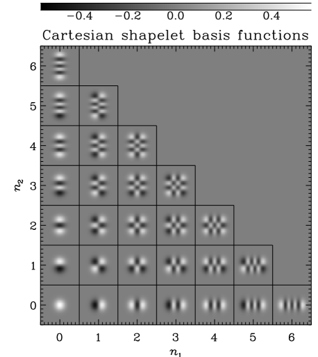
| (2) |
where is a Hermite polynomial of order , and is the shapelet scale size. These Gauss-Hermite polynomials form a complete and orthonormal basis set; this ensures that the shapelet coefficients for any image can be simply and uniquely determined by evaluating the “overlap integral”
| (3) |
In practice, a shapelet expansion (eq. 1) must be truncated at a finite order . The array of shapelet coefficients is sparse for typical galaxy morphologies, which therefore can be accurately modelled using only a few coefficients. As shown in Shapelets I, data compression ratios as high as 60:1 can be achieved for well resolved HST images. Note however, that our choice of Gauss-Hermite basis functions was not governed by the physics of galaxy morphology and evolution but by the mathematics of image manipulation. As we shall see throughout this paper, a shapelet parameterization is mathematically convenient for many tasks common in astronomy and other sciences.
2.2 Polar shapelet basis functions
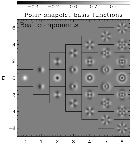
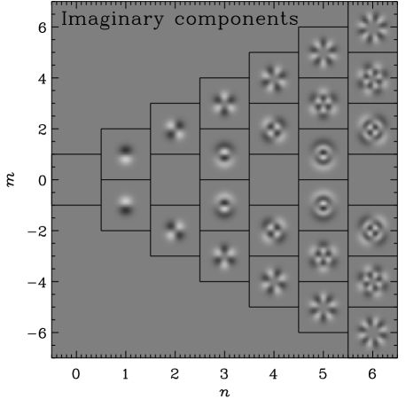
Polar shapelets were introduced in Shapelets I as an orthogonal transformation of the Cartesian basis states, and were independently proposed by BJ02. They have all the useful properties of Cartesian shapelets, and a similar Gaussian weighting function with a given scale size . However, the polar shapelet basis functions are instead separable in and . This renders many operations more intuitive, and makes polar shapelet coefficients easy to interpret in terms of their explicit rotational symmetries.
The polar shapelet basis functions are also parameterized by two integers, and , and a smooth function in polar coordinates may be decomposed into
| (4) |
The polar shapelet coefficients are again given by the “overlap integral”
| (5) |
BJ02 showed that the “polar Hermite polynomials” , which were described in Shapelets I, are related to associated Laguerre polynomials
| (6) |
for by
| (7) |
Here and are any non-negative integers. In this paper we shall instead prefer the simpler , notation, where and . In this scheme, can be any non-negative integer, and can be any integer between and in steps of two. We truncate the series at . Although the only allowed states are those with and both even or both odd, this condition will not be written explicitly alongside every summation for the sake of brevity.
As plotted in figure 2, the dimensionful polar shapelet basis functions are therefore
| (8) |
These are different from the Laguerre expansion used by BJ02 in two ways. Those are the complex conjugate of our basis functions: i.e. their is equivalent to our . The Laguerre expansion in BJ02 is also normalised by one less factor of . This dimensionality ensures that, as in the case of Cartesian shapelets, the polar shapelet basis functions are orthonormal
| (9) |
as well as complete (see e.g. Wünsche 1998)
| (10) |
where is the Kronecker delta and the asterisk denotes complex conjugation. Only those basis functions with contain net flux.
| (11) |
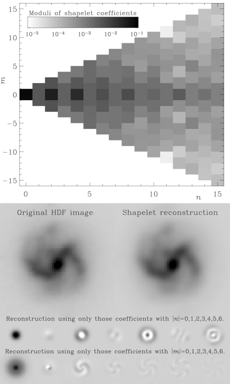
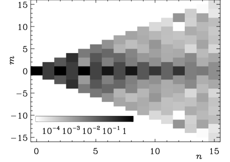
Figure 3 demonstrates the polar shapelet decomposition of a galaxy found in the HDF. The original image (middle left panel) agrees well with the reconstruction using . The top panel shows the modulus of the polar shapelet coefficients as function of the and indices. The dominant coefficients have small values of both indices, demonstrating the compactness of a polar shapelet representation, and further improved prospects for data compression. The bottom panel shows the reconstruction of the galaxy using only coefficients with given values of or , thus highlighting the contributions of terms with specific rotational symmetries. The off-central bulge is captured in the coefficients, and the main spiral arms in the coefficients. The spiral arms can also be seen as the rotation of the -only reconstructions with increasing radius. The fainter spiral arms appear as an interplay of the and 5 coefficients.
2.3 Conversion between Cartesian and polar shapelets
Cartesian shapelets are real functions, but polar shapelet basis functions and coefficients are both complex. However, their symmetries
| (12) |
simplify matters somewhat if we are concerned only with the representation of real functions , like the surface brightness of an image. Equations (9) and (12) imply that is real if and only if
| (13) |
Coefficients with are thus wholly real. All polar shapelet coefficients are paired with their complex conjugate on the other side of the line . Therefore, even though the polar shapelet coefficients are generally complex, the number of independent parameters in the shapelet decomposition of a real function is conserved from the Cartesian case.
A set of Cartesian shapelet coefficients with can be transformed, into polar shapelet representation with , using
| (14) | |||
| (19) |
The particular choices of truncation scheme for Cartesian and polar shapelets now make sense as a way to keep this mapping one-to-one.
3 Choice of shapelet scale size
A shapelet decomposition requires values for the scale size and for the centre of the basis functions to be specified in advance. Choosing the centre is relatively easy: there are many methods well-known in the astronomical literature to accurately determine astrometry from the flux-weighted moments of objects. However, the selection of is a less well-posed problem. In this section, we shall first use some properties of polar shapelets to describe the effect that the choice of the scale size has upon a shapelet decomposition. We shall then set quantitative criteria for the selection of in arbitrary galaxy images that we can implement in a practical algorithm.
Note that the selection of will be linked to the selection of . As shown in Shapelets I §2.4, these two parameters determine the maximum extent and finest resolution that can be successfully captured by a shapelet model. If , any object can be represented using any scale size . But if the shapelet expansion is truncated at finite , the shape information needs to be more efficiently contained within fewer coefficients. It is clearly desirable in this situation to select a scale size that compresses information, and lets us store the smallest possible number of coefficients.
3.1 Radial profiles
Our discussion can be simplified by initially considering only the radial profile of an object, thus reducing the task to a one-dimensional problem. Let us consider an object with surface brightness . The object’s radial profile is its brightness averaged in concentric rings about its centre, i.e.
| (20) |
With the object decomposed into polar shapelets as in equation (5), it is easy to show that this is given by
| (21) |
This simple expression results from the fact that only the basis functions are invariant under rotations. These are given by
| (22) |
The first few rotationally-invariant basis functions are written explicitly in table 1.
As a concrete example, we consider the decomposition of galaxy images from the Hubble Deep Fields (Williams et al. 1996, 1998). The mean radial profile of spiral galaxies is typically exponential, , with some characteristic radius scale . Figure 4 shows the shapelet reconstruction of an exponential radial profile using various values of , with and the integral in equation (5) calculated numerically.
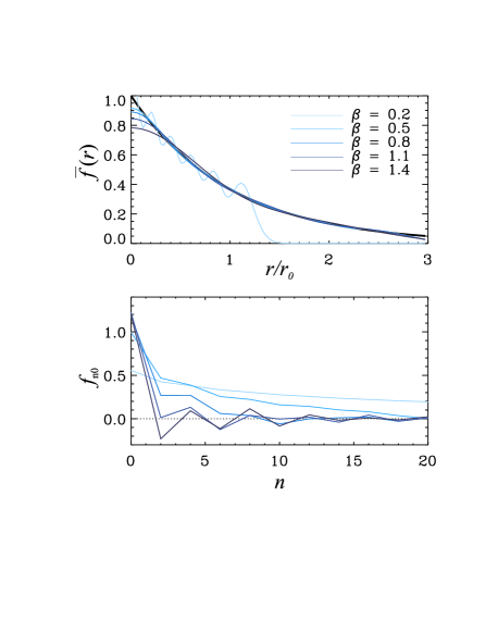
As can be seen in the top panel of figure 4, the quality of the reconstruction depends on the choice of . For small values () the reconstruction is oscillatory and cuts off the profile at large radii (). For large values (), the reconstruction fails to reproduce the cusp at small radii () and exceeds the true profile at . However, for intermediate values (), the reconstruction is good throughout the range . This range can of course be expanded by including more shapelet coefficients of higher order. As , the input model can be recovered with arbitrary precision using any value of .
The corresponding behaviour in shapelet space is apparent in the bottom panel of figure 4. The coefficients can be thought as the profile of the galaxy in shapelet space or the “shapelet profile”. For low values of the shapelet profile is very flat, showing that the power is distributed almost evenly throughout all orders. For , the coefficients are seen numerically to be . This will be an important result for the convergence of shape estimators formed from series of shapelet coefficients in §6. Convergence is fastest at , with . For higher values of , the signs of begin to alternate, and the convergence once more falls below at .
Figure 5 demonstrates the importance of a proper choice of the parameters and for the practical decomposition of spiral galaxy in the HDF. Its spiral arms complicate measurement, but its radial profile is approximately an exponential with a scale length of (12 pixels). The left column shows the growth in complexity of a shapelet model using increasing . Note in particular the rotation of the core ellipticity as is increased from 2 to 8 and higher order moments are included to resolve the spiral arms. In this column, is allowed to vary in order to minimise the least-squares difference between the model and the HDF image, shown at the bottom. The middle column shows shapelet decompositions at fixed , with varying . The residuals are plotted in the right hand column. As in figure 4, we find that the best overall image reconstruction uses . This is perhaps at the low end of the range suggested by figure 4 because of the extra high-frequency detail contained in the spiral arms.
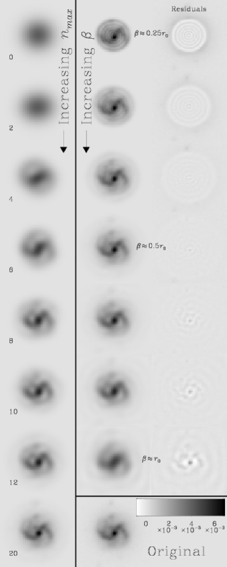
By experimentation we have found a fairly wide range of values that produce a faithful shapelet reconstruction. The information is then concentrated into the few lowest shapelet states, with fast convergence to the final model, and truncation is possible at a computationally acceptable value of . We shall now consider ways to formalize this process, and hone our choice of , and using quantitative criteria.
3.2 Existing optimisation methods
Methods in the literature that face similar choices suggest several distinct philosophies for the quantitative selection of parameters equivalent to , and . The suggestions, outlined below, differ both in the goals set for for an ideal decomposition and the method used to achieve it.
-
•
Shapelets I suggested a geometrical argument using , : the minimum (PSF or pixel) and maximum (entire image) sizes on which information exists. This could be iterated using functional rules on and as defined by shapelet coefficients. However, the coefficients change as a function of , and it is not clear what the rules should be.
-
•
Van der Marel & Franx (1993) fit 1D Gauss-Hermite polynomials to spectral lines. They arbitrarily fix , probably finding this sufficient because their spectra have relatively high S/N and their lines have a nearly Gaussian profile. Parameters equivalent to and are obtained from the best-fitting Gaussian. This also determines and in 1D is equivalent to constraining , i.e. the derivatives of the Gaussian with respect to and . The number of variables is reduced and the problem rendered tractable. Unfortunately, this does not help us in 2D because while both can be forced to zero by varying , no unique recipe can be found for setting the three states using only one value .
-
•
Van der Marel et al. (1994a,b) relax the constraint on . This is an improvement since is only the first term of an expression for the centroid, expanded using all odd in equation (56). Without the higher order corrections, the true object centroid is moved slightly from the origin: amongst other things rendering rotations and shear operations more complicated. Instead, they set from the theoretical rest wavelength of a line. Unfortunately, astrometric calibration clearly cannot be done with such accuracy. Nor has the problem been solved.
-
•
Kaiser, Squires & Broadhurst (1995) combine fitting with a stand-alone object detection algorithm, hfindpeaks. Translated into shapelet language, their approach is roughly equivalent to placing at data peaks then finding a width such that signal-to-noise ratio in is maximised.
-
•
Bernstein & Jarvis (2002) propose a similar approach. They prescribe by requiring , while moving to ensure . Higher coefficients are then determined afterwards by linear decomposition. To first order, this constraint is equivalent to that for hfindpeaks. This is generally larger than values chosen by our method below, and it can be several times larger for a high signal-to-noise object containing lots of substructure like the galaxy in figure 3. This method may indeed prescribe the optimal decomposition for weak lensing as the shear signal in the quadrupole moments becomes concentrated in one number; however, a predisposition towards particular states often leads to poor overall image reconstruction and PSF deconvolution, so it is not necessarily ideal for all applications.
-
•
Kelly & McKay (2004) were able to set a fixed physical scale of 2kpc for galaxies in the Sloan Digital Sky Survey, where photometric redshifts were available. However, galaxies have a broad distribution of physical sizes, and it may in fact become more difficult to interpret a shapelet model derived using this method.
-
•
Marshall (in preparation) describes a fully Bayesian approach to applying the shapelet transform in the context of image reconstruction. Here, , and are varied in order to maximise the evidence (the probability of observing the data, marginalised over all shapelet coefficients). At high S/N, this method gives a value of which approaches the same as that from our method below, but otherwise tends to prefer a fractionally larger , conservatively eliminating some ‘noise’ in favour of a smoother image reconstruction. However, this is computationally slow, a serious issue when analysing large images.
3.3 Optimisation of image reconstruction
We shall adopt a choice of and that is suitable for many applications, including overall image reconstruction and PSF deconvolution. Different models will be quantitatively compared via the overall reconstruction residual
| (23) |
where is the observed image, and the reconstructed image from the shapelet model. is the covariance matrix between pixel values, i.e. its diagonal elements are the noise variance in each pixel. We will need to know this a priori, or estimate it from blank areas of the image. is the number of pixels in the observed image, and is the number of shapelet coefficients used in the model. The residual itself has variance (Lupton 1993)
| (24) |
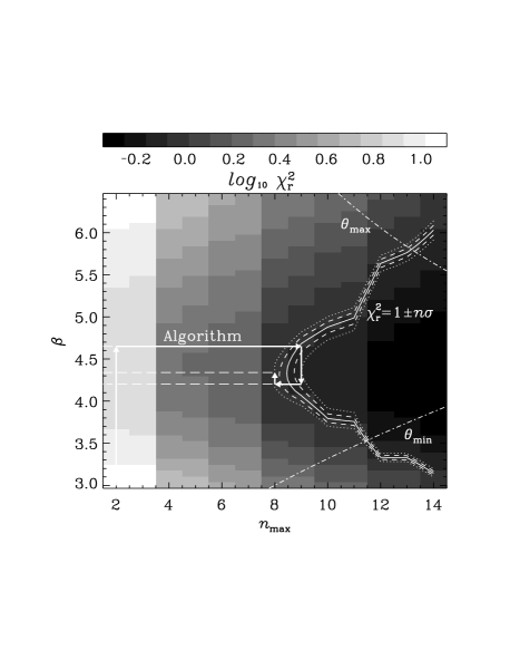
An example of typical isocontours on an plane is shown in figure 6 for an elliptical galaxy from the HDF. The horizontal trough is present for all galaxies (and many other isolated objects). This demonstrates that there is indeed an optimum for the reconstruction of this image. As one might expect, it is roughly independent of , but decreases very slightly as more coefficients are added. By increasing , the reconstruction can be improved to arbitrary precision. However, stopping at the contour produces a model whose residual is consistent with the noise. Additional coefficients would just model the background noise and should be excluded.
The form of these typical contours thus suggests a unique location in parameter space. We will choose and so that the model lies at the intersection of the trough and the contour, i.e. at the left-most point on the contour. To achieve this, we set quantitative goals of
| (25) |
| (26) |
and
| (27) |
The first constraint ensures that the scale size is well-suited to efficiently model the image. The second ensures that the shapelet center matches the object centroid. The third guarantees that sufficient coefficients () are included to model an object, but with truncation that ’smooths over’ observational noise. A flatness constraint is also included (in the right hand side of equation 27). This is particularly important for galaxies with a near neighbour or for very faint objects that have noisy and fragmented contours. In these cases, including additional shapelet coefficients may not significantly improve a fit, so the series is truncated early.
We apply extra geometrical constraints to the minimum and maximum scales of the decomposition, to prevent the model from containing features smaller than the pixel scale or extending off the edge of an image, where it would be unconstrained.
3.4 Automatic optimisation algorithm
Satisfying the three conditions (25), (26) and (27) would ensure that a shapelet decomposition uses the optimum values of , and . It is easy to determine the values of these parameters once the entire plane has been examined, as in figure 6. However, this is a slow process, so we need a practical algorithm to more efficiently explore this parameter space, and to iterate rapidly towards our targets. The numerical implementation of this iteration will inevitably be non-trivial, because it combines both minimisation and root finding, in a space with one axis discrete. Here we describe a code that we have developed to repeatedly decompose an object into shapelets, test the residual, and improve the decomposition parameters. Its stepwise approach is shown in figure 6, and the full code can be downloaded from the world wide web.
Objects are first detected in an image using SExtractor (Bertin & Arnouts 1996), a friends-of-friends peak-finding algorithm. After experimenting on various data sets, we have found the results of SExtractor highly sensitive to input settings. To avoid reliance upon these setting, we use SExtractor as sparingly as possible. We set low detection thresholds in order to obtain a complete catalogue, and filter out false detections later. We use the measurement of each object’s FWHM to make an initial guess at , and also to set the size of the fixed, circular “postage stamp” region that is extracted around each object. We aim for a postage stamp large enough to contain the entire object, but small enough to isolate it from its neighbours and to make the routine computationally efficient. We then use the SExtractor segmentation map to identify pixels in the postage stamp but well away from any object. These are used to estimate the background noise level, or to locally renormalise the pixel weight map. Within reasonable limits, the process is stable with respect to such parameters and we shall not be too concerned as to the exact SExtractor settings.
Using constant for speed, is varied in order to minimise and satisfy the criterion in equation (25), via a 1D version of the Numerical Recipes AMOEBA routine: crawling vertically in figure 6. During each step of this iteration, the centroid is simultaneously shifted to re-zero the series in equation (56) in the shapelet coefficients and thus satisfy the criterion in equation (26). Since the calculation of the centroid is independent of for isolated objects (see §7), this part of the iteration is both stable and fast. Figure 6 also shows the additional geometrical constraints of pixel and not falling off the edge of the postage stamp. These act as hard boundaries to the region of parameter space that the amoeba is allowed to explore.
Once the optimum has been found, is increased until the criterion in equation (27) is satisfied: crawling horizontally in figure 6. The increases are done in steps of two, because even states frequently improve the fit more than odd states (primarily due to the additiona of a new circular state). The value of is fine-tuned to the exact best value at the end. If two values of both allow a decomposition with , the lower value is taken.
If the object warranted more coefficients than the initial guess of , and are again readjusted at the new , using our 1D AMOEBA routine. Another search then starts back at and increases again in steps of two. The algorithm terminates when either the horizontal or vertical search returns to the value it started with. All three conditions in equations (25), (26) and (27) have then been met. Computation time for each object increases . On a single 2Ghz processor, our algorithm takes about 45 minutes to process all of the 3596 objects detected in the HDF North.
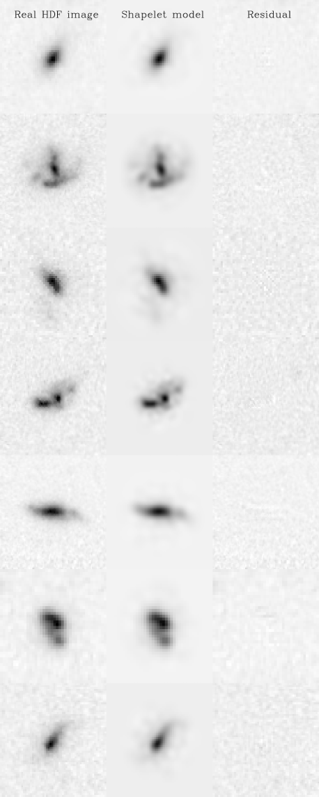
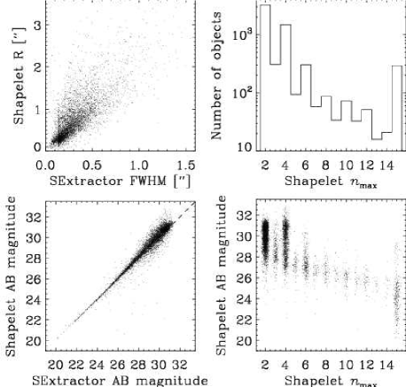
A selection of reasonably bright HDF galaxies is shown with their shapelet models in figure 7. The right-hand column shows the reconstruction residuals, which are consistent with noise even for irregular galaxy morphologies. A comparison of their shapelet-based shape estimators to traditional SExtractor measurements is shown in figure 8.
4 Decomposition of real data
4.1 Least squares fitting
Unlike the continuous, analytic formalism presented in §2, real images are complicated by pixellisation, PSF convolution and noise. In order to incorporate these effects, we shall first adopt a somewhat different approach to shapelet decomposition than the overlap integrals (3) and (5). We shall instead fit shapelet coefficients to the data using a least-squares method. Since the model in equation (23) is linear in the shapelet coefficients, we can solve for the minimum solution (23) exactly. We obtain (see Lupton 1993; Chang & Refregier 2002)
| (28) |
where is a vector of the derived shapelet coefficients, the surface brightness in each pixel arranged as a data vector, the covariance matrix between pixel values and is a matrix of each shapelet basis function evaluated in each pixel. A fit achieving has successfully modelled all significant spatial variation in the image, and removed observational noise.
If the noise per pixel is known, confidence limits can be derived on all of the assigned coefficients using this fitting method (Lupton 1993). If a complete pixel noise map is available (e.g. from multiple exposures stacked using DRIZZLE software – Fruchter & Hook, 2002), it can be used to down-weight noisy pixels where cosmic rays or hot/cold pixels were present in some of the exposures. Although the code available on the world-wide web simply uses a diagonal matrix for that contains only the noise level in each pixel, the method is, in general, able to use the full covariance matrix that contains the amount of covariance between different pixels. In real data, the flux in adjacent pixels is indeed slightly correlated because of convolution with the PSF and also because of additional aliasing effects introduced by DRIZZLE. If this effect is important, the pixel-to-pixel covariances could be estimated from empty regions of an image and included in the calculation. In particular, this may have a small improvement on statistics measured from very small objects (c.f. Massey et al. 2004).
A constant background level can also be removed using this method, by adding an undetermined constant to the set of basis functions. Poor flat fielding or local background gradients near a bright object can also be fit and removed by adding a plane with variable slope. Although these functions are not strictly orthogonal, the procedure works well in practice as long as there are sufficient pixels around the fitted object that contain only background noise.
4.2 PSF deconvolution
All real images are inevitably seen after convolution with a Point Spread Function (PSF). In astronomy, this is typically caused by atmospheric turbulence or “seeing” (for ground-based observatories), aperture diffraction at the primary mirror, and imperfect telescope tracking or optics. The combination of such effects can be measured from the size and shape of stars observed in an image (because these distant objects would be point-like in the absence of a PSF), and can be fit with a shapelet model in the same way as the galaxies. Shapelets I presented the matrix operation for convolving an image with a Gaussian PSF in shapelet space. Shapelets II extended this derivation to a general PSF and demonstrated PSF deconvolution via matrix inversion. However, the inversion of the PSF matrix is potentially slow and may be numerically unstable. Our least-squares fitting method will allow us to elegantly sidestep this process by convolving the basis functions with the PSF model in advance, then fitting this new basis set to the data. The returned shapelet model, reconstructed using the unconvolved basis functions, will be automatically deconvolved from the PSF.
The formalism for convolution in shapelet space is presented in Shapelets I §4 and involves three separate scale sizes for three separate objects: for the unconvolved model, for the PSF, and for the convolved model (there are also corresponding values of , and ). We assume that is known. We can optimise as in section §3.3. However, the choice of is a matter entirely internal to the fitting procedure. Just as before, if , any will work (but this time without increasing the number of external free parameters in the model). In practice, however, it is still necessary to truncate this series somewhere. Note that was incorrectly suggested as a “natural choice” for this parameter in Shapelets I. Another choice would be , which, with , makes the convolution matrix symmetric and thus simplifies its calculation.
The optimum values for and are in fact obtained from an argument concerning the information present in shapelet coefficients. A shapelet model contains information only between a minimum and maximum scales
| (29) |
During convolution, and add in quadrature to produce ; and add similarly to produce ; the range of scales on which information is available decreases or remains constant. Values of and can be chosen to most efficiently capture the information contained between the new scales. Writing as etc. for brevity, we find
| (30) |
and
| (31) |
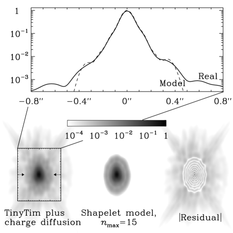
The PSFs of cameras on board the Hubble Space Telescope are well known and stable. Figure 9 shows an oversampled TinyTim (Krist 1997) model of the Wide-Field Planetary Camera 2 (WFPC2) PSF, raytraced through an engineering model, plus charge diffusion to simulate photon capture within the CCD cameras. This is easy to model with shapelets, except for the fact that its steep cusp and extended wings are intrinsically ill-matched to the Gaussian around which shapelets are constructed. The PSF is shown in the figure beside a shapelet decomposition up to . This is sufficient to accurately capture the core and the first two diffraction rings, which are already more than two orders of magnitude below the maximum, but does not extend to the four faint diffraction spikes or far into the low-level wings (note that the colour scales are logarithmic). In principle, this could be further extended at a cost to processor time by using more shapelet coefficients.
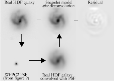
Figure 10 demonstrates successful PSF deconvolution. A galaxy from the HDF is convolved with the WFPC2 PSF (in real space). This is treated as the observed image, and deconvolved from the PSF using a shapelet fit. The resulting reconstruction is in good agreement with the original galaxy image, as can be seen from its small residual. Note that the optimum scale size for the model is slightly lower when PSF deconvolution is performed. This reflects the need to capture finer details.
4.3 Pixellisation
Real image data is typically stored in discrete pixels. To link this to the analytic shapelet formalism, one must either smooth the data or pixellate the shapelet basis functions. Smoothing the data requires an arbitrary interpolation scheme to be defined, and resampling the data onto smaller pixels can be very slow. A better approach is to leave the data alone, and discretize the smooth shapelet basis functions. This reduces the integrals in equations (3) and (5) to sums over pixel values, which are fast to compute. However, they are no longer analytically exact. We therefore need to define a discretization scheme that keeps the basis functions as orthogonal as possible, and the integrals as accurate as possible.
As pointed out by Berry, Hobson & Withington (2004), one cannot simply adopt the value of basis functions at the centre of each pixel. Basis functions that contain oscillations on scales smaller than the pixel size are sampled in an essentially random manner. Their discrete versions are then neither representative of the analytic function nor orthogonal. Degeneracies are introduced between shapelet coefficients during the decomposition that unstabilise the inversion of coefficient matrices in the reconstructed model, and bias quantities like an object’s flux. Fortunately, this is rarely a problem in practical cases, because we can choose and in advance to isolate only those basis functions that contain oscillations on scales larger than the pixel (or seeing) size. Under these conditions, Berry, Hobson & Withington (2004) show that the shapelet basis functions are indeed orthogonal.
We suggest an even safer alternative here. The Cartesian basis functions are separable in and , and may be analytically integrated within rectangular pixels. This is exactly the same process undergone by photons arriving at a CCD, where the smooth function of a real scene gets binned into digital squares. Once we have convolved the basis functions with the PSF, and integrated them within pixels, they can be suitably matched to the data.
To integrate the 2D Cartesian basis functions, first consider the 1D basis functions from Shapelets I,
| (32) |
Integrating by parts and using two well-known identities (see e.g. Boas Ch. 12)
| (33) |
and
| (34) |
one can obtain the recurrence relation
| (35) | |||||
| (36) |
Finally, note that
| (37) | |||||
| (38) |
This supplies all the necessary integrals. Since the 2D Cartesian basis functions are separable in and , it is easy to extend this derivation to integrate within square CCD pixels:
| (39) |
where, if there is no ‘dead zone’ around the edge of a pixel, is the angular size of a pixel. A missing pixel border, due for instance to electronics which is unresponsive to light, can be included by altering the limits on the integral.
We can either use this result to obtain a model in Cartesian shapelet space, which can later be converted to a polar shapelet representation using equation (14), or we can integrate the polar shapelet basis functions within pixels using the same equations. This integration is a particularly important advance for small galaxies or for shapelet basis functions at high-, that can contain oscillations smaller than a single pixel.
5 Coordinate transformation
Image manipulation via linear transformations is simple in shapelet space. As in Shapelets I, let us consider an infinitesimal coordinate transformation , where is a displacement and is a matrix parametrized as
| (40) |
The parameters , , and correspond to infinitesimal rotations, dilations, translations and shears.
An image transforms as , which can be written as
| (41) |
where , , and are the operators generating rotation, convergence, shears and translations, respectively. We adopt a notation from weak gravitational lensing, where a “convergence” corresponds to a change in an object’s radius by a factor . These transformations can be viewed as a mapping of coefficients in shapelet space. For example, a finite rotation is
| (42) |
so a rotation through can be written as
| (43) |
An (infinitesimal) dilation can be performed in polar shapelet space by mapping the shapelet coefficients as
The shapelet model may require more coefficients after this transformation. Note that this dilation operation increases both the flux and the image area by a factor , thus conserving surface brightness. To instead perform a dilation that conserves the total flux, divide the right hand side of equation (5) by this factor. To first order, this is
In §6, we shall ensure that shape estimators for a shapelet model are independent of the scale factor chosen for the decomposition by ensuring that the estimators are unchanged under this mapping.
Rather than these first-order approximations, finite dilations can be performed to all orders using the rescaling matrix in the appendix of Shapelets I. This is identical to the convolution matrix, but the image is convolved with a -function.
Shears and translations can be performed using
| (46) | |||
and
| (47) | |||
with the translation specified in units of .
Other image manipulations can also be represented as mappings of shapelet coefficients. Changes of flux by a factor are trivially implemented by the mapping
| (48) |
It is also possible to circularise an object with the mapping (see §3.1)
| (49) |
or to flip an object’s parity by reflection in the -axis using
| (50) |
Combining this with the rotation operator allows reflections to be performed in any axis.
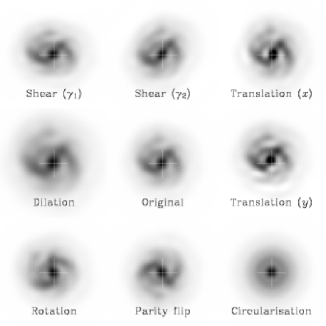
These operators’ actions are demonstrated upon a real galaxy image in figure 11.
6 Object shape measurement
The above symmetries of the polar shapelet basis functions can be used to identify combinations of shapelet coefficients that measure an object’s flux (photometry), centroid position (astrometry) and size. Similar weighted combinations of Cartesian shapelet coefficients were found in Shapelets I, but we find the interpretation of polar shapelets more intuitive, and the expressions below are usually more simple than their Cartesian equivalents. For example, the rotationally invariant part of an object is isolated into its coefficients. The linear offset of an object from the origin is described by its coefficients and the ellipticity of an object by its coefficients. In the latter cases, the magnitude of the coefficients indicate an amplitude, and the phases a direction.
6.1 Photometry
Practical measurements of objects’ flux usually introduce a Gaussian or top-hat weight function in order to limit contamination from surrounding noise and nearby objects. The flux of a shapelet model inside a circular aperture can be calculated using only the coefficients with . All other coefficients correspond to basis functions with positive and negative regions that cancel out under integration around . From equations (21) and (22) for an object’s radial profile, we find that
| (51) |
where
| (52) |
Using relation (77) to integrate by this parts, we can find a recursion relation111Thanks to Mark Coffey for help deriving this expression.
| (53) |
and a closed form
| (54) |
However, the imposition of a integration boundary is unnecessary with shapelets because the model is analytic and noise-free. In the limit of , we obtain a simple expression for the total flux in a shapelet model
| (55) |
a result that can also be recovered by transforming the sum over Cartesian shapelet coefficients from Shapelets I into polar shapelet space via equation (14). Cartesian shapelet models can also be integrated within square apertures using equations (35) to (39).
This extrapolation to large radii does rely upon the faithful representation of an object by a shapelet expansion, and the removal of its noise via series truncation. Such truncation restricts the basis functions’ completeness, and a weight function (constructed from a combination of the allowed basis functions) akin to a “prior probability” is subtly implicit inside our fitting procedure. However, a fitting method like ours can beat a direct, pixel-by-pixel measurement. Our fit is able to include flux from the extended wings of an object, by integrating it over a large area, even when the signal lies beneath the noise level in any individual pixel. The wings of galaxies in figure 7 are indeed well-captured by the shapelet models.
6.2 Astrometry
It can similarly be shown that the unweighted centroid () is
| (56) |
Here the summation is over only odd values of , because only these have the coefficients that possess the desired rotational symmetries.
6.3 Size
Measures for the size and ellipticity of an object can be derived from its unweighted quadrupole moments,
| (57) |
The rms radius of an object is given by
| (58) | |||||
| (59) |
6.4 Ellipticity
The unweighted ellipticity of an object can also be calculated from its quadrupole moments.
| (60) |
where the complex ellipticity notation of Blandford et al. (1991), with , arises here naturally.
7 Galaxy morphology classification
The shapelet decomposition of an object captures its entire structure, and useful information is frequently found in coefficients of higher order than those considered above. In particular, galaxy morphologies are well known to provide an indication of their physical properties, local environment and formation history. The classical “Hubble sequence” of morphological types has been recently improved by several shape estimators that attempt to classify galaxies in a more quantitative manner, which correlates directly with the physical properties of interest (e.g. Simard 1998; Bershady, Jangren & Conselice 2000; van den Bergh 2002).
It is possible to manufacure such morphology diagnostics from weighted combinations of shapelet coefficients. Introducing shapelets to this field allows a measurement to take advantage of our robust treatment of noise, pixellisation and PSF deconvolution. The shapelet expressions for existing shape measures are frequently elegant; and the natural symmetries in shapelets also suggest new diagnostics.
7.1 General scale-invariant quantities
One approach is to consider general shape estimators , formed from a linear combination of shapelet coefficients, as an extension of the previous section
| (61) |
where are arbitrary weights, and the exponent sets the dimension of the estimator. These are also linear in a galaxy’s surface brightness. We initially restrict ourselves to using those combinations which are independent of to at least first order. This ensures that the choice of the scale factor does not affect the final result, and is also equivalent to invariance under object dilations (5). We can then impose further constraints that the estimator must be independent of or linearly dependent upon the various other operations described in §5. Setting and using the result that
| (62) |
it is easy to show that we require
| (63) | |||||
Notice that all quantities so formed mix coefficients with only one value of . This can be chosen to give the desired properties under rotation. Any term on the right-hand side should be ignored if it refers to non-existent states with negative . The normalisation of the first term in each series, , is arbitrary: this can be set to ensure independence to changes of object flux.
Setting and recovers the flux , centroid , rms square radius and ellipticity , up to the normalisation factor of for the latter three quantities. This proves that these are indeed the only -invariant linear quantities with such dimensionality and rotational symmetries. Furthermore, since equations (55), (56), (59) and (60) describe for unweighted moments, they must in fact be independent of to all orders.
All of these basic shape estimators converge for any galaxy with a shapelet spectrum steeper than . This includes both spiral galaxies with an exponential profile, and elliptical galaxies with a “de Vaucouleurs” profile, as long as is kept sufficiently low to prevent the high- coefficients from modelling background noise at large radii. The flux and centroid estimators converge most rapidly, so are least sensitive to the choice of . The error on these series due to truncation can be calculated using any of a range of methods for generic Taylor series in e.g. Boas (1983).
7.2 Concentration
We can extend this sequence by raising further. For example, setting and gives the 2D unweighted kurtosis of the image, producing an estimate of the object’s concentration. Unfortunately, such a high value of yields a series of shapelet coefficients that does not converge for galaxies with a de Vaucouleurs or exponential radial profile.
We have also noticed that a ratio of the two existing shapelet scale sizes, and , also works rather well as a concentration index (although this estimator is not independent of ). Further work will need to be done to calibrate this estimator to the physical properties of galaxies.
An alternative approach is to mimic pre-existing, and pre-calibrated, morphology diagnostics. Bershady, Jangren & Conselice (2000) define a concentration index
| (64) |
where and are the radii of circular apertures containing 80% and 20% of the object’s total flux. This correlates well with a galaxy’s Hubble type (Bershady, Jangren & Conselice 2000) and also its mass (Conselice, Gallagher, & Wyse 2002). Integrals (51) to (6.1) can be evaluated for various values of , to find and , and thus calculate this quantity for a shapelet model.
7.3 Asymmetry
Conselice, Bershady & Jangren (2000) define an asymmetry index
| (65) |
where the superscript denotes an image rotated through . A term dealing with the background noise and sky level has been omitted here, as these are automatically dealt with during the shapelet decomposition process in §4. Asymmetry correlates with a galaxy’s star formation rate (Conselice, Bershady & Jangren 2000), and high asymmetry values often indicate recent galaxy interactions or mergers.
In a shapelet expansion, all of the information about galaxy asymmetry is contained in coefficients with odd (and ). Using the orthonormality condition (9) and rotating via equation (43), we find the simple form
| (66) |
Estimators of asymmetry under rotations of or can also be formed from sums of shapelet coefficients with not divisible by 3 or 4 respectively.
7.4 Chirality
A quadratic combination of shapelet coefficients can be used to describe the “chirality” or “handedness” of an object. One dimensionless estimator can be formed for each value of , to trace the relative rotation of those coefficients, with increasing . This is roughly equivalent to tracing the rotation of a galaxy’s isophotes with increasing radius. For example, the galaxy shown in figure 3 has two prominent spiral arms that unwind in a clockwise sense, so it has a large, positive value of .
We require that the chirality estimators should be invariant under global rotation of the object; invariant under changes of flux; invariant to first order under changes of ; and to flip sign when the object is mirror-imaged. These conditions uniquely specify
| (67) |
where and
| (68) |
thus mixing all coefficients with the same value of .
This estimator has yet to be calibrated against physical quantities. However, this approach ought to be able to automatically distinguish between elliptical galaxies and spiral galaxies in way that mimics a visual classification, and could also be adapted as a function of to find bars in the cores of spiral galaxies.
8 Conclusions
We have extended the formalism of shapelets for image analysis from basis functions separable in Cartesian to polar coordinates. Cartesian shapelets are convenient for the initial object decomposition. In particular, we have shown that that they can analytically be integrated inside a square boundary, thus facilitating the pixellisation of the smooth basis functions. On the other hand, polar shapelets decompose an object into components with explicit rotational symmetries, and often have a more direct physical interpretation. In addition, they yield more compact representations of typical galaxy images, since terms with low orders of rotational symmetry tend to dominate.
We have quantitatively investigated the effects of the choice of the shapelet scale size parameter, . For most objects in astronomical images, one scale size is clearly optimal for high quality image reconstruction, data compression and the fast convergence of shape estimators. We have developed a practical algorithm to find this value of for arbitrary objects in real images, plus optimum values for the shapelet centre and truncation order . This algorithm can also take into account observational effects including noise, pixellisation and PSF deconvolution.
We have then described a number of applications of polar shapelets. Shapelet models can be rotated, enlarged and sheared by simple analytic operations. Since the shapelet basis functions are invariant under Fourier transform, analytic convolutions and deconvolutions (e.g. from a PSF) are also easy to perform. Linear combinations of an object’s polar shapelet coefficients produce elegant expressions for its flux (photometry), position (astrometry) and size. We also showed how other combinations of shapelet coefficients can be used to distinguish between morphological types of galaxies. A complete IDL software package to perform the image decomposition and shapelet image analysis is publicly available on the world wide web at http://www.astro.caltech.edu/rjm/ shapelets/.
Acknowledgments
The authors thank David Bacon, Gary Bernstein, Sarah Bridle, Tzu-Ching Chang, Mark Coffey, Chris Conselice, Phil Marshall and Jean-Luc Starck for invaluable insights and constructive conversations. Astute suggestions from the referee helped shape this paper into a more logical progression.
References
- [1] Bernstein G. & Jarvis M. 2002, AJ 123, 583 (BJ02)
- [2] Berry R., Hobson M. & Withington S. 2004, MNRAS 34, 199
- [3] Bershady M., Jangren A. & Conselice C. 2000, AJ 119, 2645
- [4] Bertin E. & Arnouts S. 1996, A&AS 117, 393
- [5] Blandford R., Saust A., Brainerd T. & Villumsen J. 1991, MNRAS 251, 600
- [6] Boas M. 1983, “Mathematical Methods in the Physical Sciences”, Wiley
- [7] Conselice C., Bershady M. & Jangren A. 2000, ApJ 529, 886
- [8] Conselice C., Gallagher J. & Wyse R. 2002, AJ 123, 2246
- [9] Chang T. & Refregier A. 2002, ApJ 570, 447
- [10] Gerhard O. 1993, MNRAS 265, 213
- [11] Goldberg D. & Bacon D. 2004, ApJ 619, 741
- [12] Goldberg D. & Natarajan P. 2002, ApJ 564, 65
- [13] Kaiser N., Squires G. & Broadhurst T. 1995, ApJ 449, 460
- [14] Kelly B. & McKay T. 2004, AJ 127, 3089
- [15] Krist J. & Hook R. 1997, “The Tiny Tim User’s Guide”, Baltimore: STScI
- [16] Lupton R. 1993, “Statistics in Theory and Practice”, Princeton U. Press
- [17] Massey R., Refregier A., Conselice C. & Bacon D. 2004, MNRAS 348, 214
- [18] Refregier A. 2003, MNRAS 338, 35 (Shapelets I)
- [19] Refregier A. & Bacon D. 2003, MNRAS 338, 48 (Shapelets II)
- [20] Simard L. 1998 in “ADASS VII”, A.S.P. conference series 145, 108
- [21] Van den Bergh S. 2002 AJ 124, 786
- [22] Van der Marel R. & Franx, M. 1993, ApJ 407, 525
- [23] Van der Marel R. et al. 1994, MNRAS 268, 521
- [24] Williams R. et al. 1996, AJ 112, 1335
- [25] Williams R. et al. 1998, A&AS 193, 7501
- [26] Wünsche A. 1998 J. Phys. A: Math. Gen. 31, 8267
Appendix A Laguerre polynomials
Different conventions have been used to define the Laguerre polynomials, especially before the 1960s. The term is omitted from equation (6) in many older books, and caution must be observed with the resulting relations. Several useful recursion relations can be derived to simplify their calculation (e.g. Boas 1983, Ch.12), which we gather here, using our convention, for future reference:
| (69) | |||||
| (70) | |||||
| (71) | |||||
| (72) | |||||
| (73) | |||||
| (74) | |||||
| (75) | |||||
| (76) | |||||
| (77) |