Non-parametric inversion of strong lensing systems.
Abstract
We revisit the issue of non-parametric gravitational lens reconstruction and present a new method to obtain the cluster mass distribution using strong lensing data without using any prior information on the underlying mass. The method relies on the decomposition of the lens plane into individual cells. We show how the problem in this approximation can be expressed as a system of linear equations for which a solution can be found. Moreover, we propose to include information about the null space. That is, make use of the pixels where we know there are no arcs above the sky noise. The only prior information is an estimation of the physical size of the sources. No priors on the luminosity of the cluster or shape of the halos are needed thus making the results very robust. In order to test the accuracy and bias of the method we make use of simulated strong lensing data. We find that the method reproduces accurately both the lens mass and source positions and provide error estimates.
keywords:
galaxies:clusters:general; methods:data analysis; dark matter1 Introduction
Analysis of strong lensing images in galaxy clusters is one of the more subjective and intuitive fields of modern astronomy (see Blandford & Narayan 1992, Schneider, Ehlers & Falco 1993, Wambsganss 1998, Narayan & Bartelmann 1999, Kneib 2002, for comprehensive reviews on gravitational lensing). The common use of parametric models means making educated choices about the cluster mass distribution, for instance that the dark matter haloes follow the luminous matter in the cluster or that galaxy profiles posses certain symmetries. Once these choices are made, one can only hope they are the right ones. The recent improvement in strong lensing data however, is impressive and should increasingly allow us to extract information using fewer assumptions. For instance, it should allow us to relax assumptions about the mass distributions of the cluster and instead enable us to test this. The approach of testing rather than assuming the underlying physics has now been used in other branches of astrophysics and cosmology (e.g. Tegmark 2002) but has so far been largely absent in strong lensing analyses.
There are two relatively different fields within the area of strong lensing, namely lensing by galaxies and galaxy clusters. These are different both in appearance as well as in abundance. Galaxy-cluster systems are few and far between, only the most abnormally dense clusters have surface densities greater than the critical density for lensing. However, they are much more spectacular than their galaxy lens counterparts. The most massive clusters are able to create multiple images of extended objects such as distant galaxies with image separations of up to arcminute. Arguably the most impressive system, A1689 (Broadhurst et al. 2005), boasts more than 100 multiple images of some 30+ sources. Galaxy lens systems are of course on a much smaller scale with image separations of a few arcseconds. They are far more abundant, but less impressive. The lensed objects that we are able to observe are typically high redshift quasars due to their high luminosity and point like structure, although galaxy-galaxy lensing has been observed ( Brainerd, Blandford & Smail 1996, Hudson et al. 1998, Guzik & Seljak 2002).
The classification of strong lensing systems into these two groups is not merely a matter of scale. The baryons in galaxies have had time to cool and form the visible galaxy, thereby giving a cuspy profile, suitable for lensing. The cooling time for galaxy clusters exceed the Hubble time and the density profile is therefore far less cuspy, making them less ideal lenses. Although cluster lens systems are scarce, the impressive number of lensed images in each system, mean they still contain a lot of information, particularly regarding cluster mass profiles. The information is harder to extract due to the relatively complicated gravitational potentials, but if this challenge can be overcome they could be highly useful probes, certainly of cluster physics and potentially also for cosmology (Yamamoto & Futamase 2001, Yamamoto et al. 2001, Chiba & Takahashi 2002, Golse et al. 2002, Sereno 2002, Meneghetti et al 2005) The intention of this paper is to improve our methods for extracting this information.
Although alternative approaches have been suggested to recover the density field in both the weak and strong lensing regime, (see for instance Kaiser & Squires 1993, Broadhurst et al. 1995, Kaiser 1995, Schneider 1995, Schneider & Seitz 1995, Seitz & Schneider 1995, Bartelmann et al. 1996, Taylor et al. 1998, Tyson et al. 1998, Bridle et al. 1998, Marshall et al. 1998), the standard approach to modeling strong cluster lenses is using parametric methods. This is motivated by the fact that the data usually do not contain more than a few arcs. This is not enough to constrain the mass distribution without the help of a parametrization. Parametric methods rely heavily on assumptions or priors on the mass distribution (Kochanek & Blandford 1991, Kneib et al. 1993, 1995, 1996, 2003, Colley et al. 1996, Tyson et al. 1998, Broadhurst et al. 2000, 2005, Sand et al. 2002). A common prior is the assumption that there is a smooth dark matter component which is correlated spatially with the centroid of the luminous matter in the cluster. The mass is then ususally modeled by a large smooth dark matter halo placed on top of the central galaxy or the centroid of the luminous matter, as well as smaller dark matter haloes located in the positions of the other luminous galaxies. The parameters of each halo are then adjusted to best reproduce the observations.
There is plenty of subjectivity involved in this process, particularly in the addition of the dominant dark matter component to the cluster. The assumption that the dark matter follows the luminosity is necessary but remains the Achilles heel of parametric lens modelling. For large clusters the number of parameters in the parametric lens model quickly becomes large but there is still no guarantee that the parametric model used, is in fact capable of reproducing well the mass distribution. It is not hard to envisage complications like dark matter substructure, asymmetric galaxy profiles, interactions between individual galaxies and the cluster or even dark matter haloes without significant luminosity all of which would not be well represented by the typical parametric methods. In these cases, where the number of parameters is large, we may want to consider alternative non-parametric methods where all the previous problems do not have any effect on any of the assumptions. Also is in these situations where the number of parameters in both parametric and non-parametric methods is comparable. When the number of parameters is comparable in both cases, it is interesing to explore non-parametric methods since they do not rely on the same assumptions.
This paper does not pretend to be an attack to parametric methods but a defense of non-parametric alternatives. Parametric methods are usually the best way to obtain information about the gravitational potential (few multiple images, simple lens) and are not affeted by resolution problems, specially in the center of the lens which can play a key role in reproducing the radial arcs. They however suffer of some potential problems, some of which have been outlined above. These problems combined with the impressive quality of recent and upcoming data lead us in this paper to explore the potential to constrain the mass distribution without imposing priors on it. In other words we want to know what strong gravitational lensing images can tell us about cluster mass profiles whilst pretending we know nothing about the luminosity. Upcoming images of strong lensing in galaxy clusters will contain of the order of a hundred arcs and should make this a manageable task (Diego et al. 2004). A non-parametric approach will provide an important consistency check, since concurring results would lend strength to the parametric approach, whereas any resulting differences would need to be addressed.
Accepting this challenge we present in this paper a new method which makes use of all the available information in super-high quality strong lensing systems. The method has also been thoroughly tested with simulated lensing data with very good results. We thus address the crucial issue of how well we can reproduce both the cluster mass profile and the positions and shapes of the background galaxies.
We want to stress that ours is by no means the first work proposing use of non-parametric methods in strong lensing. Among the non-parametric methods already available, are the pixellization methods of Saha et al. (1997, 2000), Abdelsalam et al. (1998a, 1998b), Williams et al. (2001), who first established many of the ideas revisited in this work, as and also the multi-pole approach of Kochanek & Blandford (1991), Trotter et al. (2000).
Naturally, our work shares many similarities with this former work, but there are also important and interesting differences. Firstly, in Saha et al. (1997) (and subsequent papers), the authors divide the lens plane into a grid similar to the method presented here, but with the important difference that their grid is fixed while our grid is dynamical. Our grid adapts to the new estimated mass at each step. This has important implications for the solution since high density regions will be sampled more heavily. These dense regions play a key role, particularly in the positions of the radial arcs. Not sampling these regions properly will necessarily lead to a biased mass distribution.
Another important difference with Saha et al (1997) is that they make use of a prior on the mass distribution, penalizing deviations from the distribution of luminous matter. They claim this prior does not play an important role but we find this questionable. It is hard to quantify the effect since the method apparently was not tested on simulated lensing data. In contrast, as mentioned above, our method is thoroughly tested with simulations to quantify how well the mass distribution is recovered. We do not use any prior other than a physical prior on the sizes of the sources. This prior is proved to be weak provided it is chosen with a minimum of wisdom.
A third important difference between the work presented in this paper and others is that we show how to speed up the algorithm significantly by adopting techniques commonly used in optimization problems.
Moreover as an added novelty, our algorithm also includes for the first time information about the null space. Rather than using only the information in the lensed arcs, we use information which has hitherto been overlooked; the areas in the sky where no arcs are observed.
The paper is laid out as follows. In the next section we present the lens inversion problem, and provide a linear approximation. We then in section 3 present the simulated lensing data used to test the method, before we go on to present the adaptive gridification of the lens-plane, section 4. In section 5 we describe the various inversion algorithms and finally, in section 6 we introduce the use of the complementary (null) space.
2 The problem formulated in its basic linear form
The fundamental problem in lens modelling is the following: Given the positions of lensed images, , what are the positions of the corresponding background galaxies and the mass distribution of the lens, . Mathematically this entails inverting the lens equation
| (1) |
where is the deflection angle created by the lens which depends on the observed positions, . From now on we will omit the vector notation unless otherwise noted. The data points of our problem, , are given by the and positions of each of the pixels forming the observed arcs.
The deflection angle, , at the position , is found by integrating the contributions from the whole mass distribution.
| (2) |
where , , and are the angular distances from the lens to the source galaxy, the distance from the observer to the lens and the distance from the observer to the source galaxy respectively. In equation 2 we have made the usual thin lens approximation so the mass is the projected mass along the line of sight . Due to the (non-linear) dependency of the deflection angle, on the position in the sky, , this problem is usually regarded as a typical example of a non-linear problem. We will see that this is only partially true.
The next approximation we make is to split the lens plane in small regions (hereafter cells) over which the projected mass is more or less constant. We can then rewrite equation (2) as;
| (3) |
The first point we want to make here is that the deflection angle may be thought of as the net contribution of many small masses in the positions , each one pulling the deflection in the direction of () and with a magnitude which is proportional to . If we divide the lens plane in a grid with cells, the masses can be considered as the mass contained in the cell (). If the cells are sufficiently small then the above pixellization of the mass plane will give a good approximation to the real mass distribution.
Our second point is that the problem is non-linear in one direction but linear in the other. That is, given a position in the sky (and given a lens) there is only one which satisfy equation 1 but given a position of the background galaxy , there may be more than one position in the sky () satisfying equation 1 or equivalently, the source galaxy may appear lensed in more than one position in the sky. The linear nature of the problem is evident when one realizes that the only non-linear variable, namely the positions, are fixed by the observation and that the problem depends linearly on the unknowns ( positions and masses, , in the cells).
Let us now assume that we have a data set consisting of a system of radial and tangential strong lensing arcs which are spread over pixels in the image. We will also assume that we know which arcs originate from the same sources. Since both the data and the mass distribution has been discretized we can rewrite equation (1) as a simple matrix equation:
| (4) |
where and are now element vectors containing and values of the observed positions and the (unknown) source positions respectively. is the mass vector containing all mass cells, and is the () matrix casting the mass vector into a vector of displacement angles. A more technical account of the make-up of the matrix can be found in the appendix.
Equation 4 clearly demonstrates the linear nature of the problem when formulated in this manner. The problem has now been reduced to a set of linear equations with unknowns (lens masses and source galaxy positions). Notice that when the problem is formulated in this form, there are more unknowns than equations which means it is an underdetermined system with an infinite number of solutions. In order to identify a suitable solution for such a system, we need to add extra information or impose constraints.
One way of doing this is by reducing the number of unknowns, for instance by removing the source positions from the unknown category. This can be achieved by minimizing the dispersion in the source plane, i.e. demanding that the pixels in the source plane be as concentrated as possible for each source. In this case we are left with only unknowns.
Another way of constraining the system is by assuming the sources are well approximated by point sources, which reduces the number of unknowns to . This means effectively demanding that all observed s for arcs corresponding to the same source, can be traced back through the lens to single points. With this assumption we can rewrite the lens equation in the compact form of
| (5) |
is now a matrix of dimension and is the vector of dimension containing all the unknowns in our problem (see appendix A), the mass elements and the central (- and ) coordinates of the sources. Now the system is matematically overdetermined (more data points that unknowns) and has a unique point source solution. This unique solution can be found by numerical methods as we will see later.
The linearization of the problem means that it is in principle solvable by both matrix inversion and simple linear programming routines. In practice, the problem quickly becomes ill-conditioned and too large for direct matrix inversion, and approximate numerical methods are more suitable. The main problem with the linearization is that we do not know if the obtained linearized solution creates artificial tangential or radial arcs. Checking this requires forward solving of the lens equation which is non-linear due to the complicated dependence of the deflection angle on .
We suggest a novel approach to this problem, by using all the available information in the images, i.e. the information inherent in the dark areas (pixels containing no arcs) as well as the observed arcs. By pixellization the dark areas, tracing these pixels back through the lens and imposing that they fall outside the sources it is possible to find the true solution without over-predicting arcs. This use of the null space is to our knowledge unprecedented, and in principle allows for a complete, linear solution to a problem usually considered non-linear.
3 Simulations
Before proceeding to invert the system of linear equations (5), it is instructive to take a closer look at the simulations which are going to be used to test the inversion algorithms. Given that most methods rely on the luminous mass distribution, this is particularly important should the galaxies not accurately trace the dark matter.
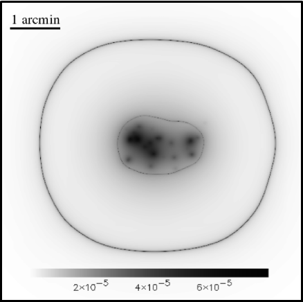
Our simulations consist of three elements. The first element of the simulation is the projected mass distribution () in the lens plane. We simulate a generic mass distribution of a cluster with a total projected mass of h-1 M⊙ in the field of view located at redshift . The field of view of our simulation is 0.1 degrees The mass profile is built from a superposition of 20 NFW profiles with added ellipticity. The halos’ masses vary from h-1 M⊙ to h-1 M⊙. In the context of lensing, NFW halos seem to reproduce well the shear profile of massive clusters up to several Mpc (Dahle et al. 2003, Kneib et al. 2003, Broadhurst et al. 2005). The final mass distribution is shown in figure 1. Also in the same figure we show the two critical curves. The interior one is the radial critical curve and the exterior one the tangential critical curve. Both curves have been calculated assuming the source is at redshift . The tangential critical curve is usually associated with the Einstein radius. Its large size (radius arcmin) is due to the unusually high projected mass of our cluster plus its relatively low redshift (). Although the deduced Einstein radius is larger than the one observed in clusters, the simulation presented here will serve the purpose of testing the different methods discussed here. More realistic simulations with proper mass distribution and source density will be presented in a future paper.
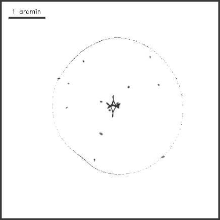
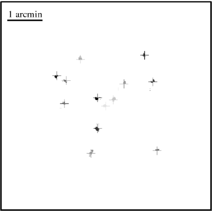
The second element in our simulation are the sources (), for which we extract 13 sources from the HUDF (Hubble Ultra Deep Field, Beckwith et al. 2003). We assign them a redshift () and size and place them in different positions behind the cluster plane.
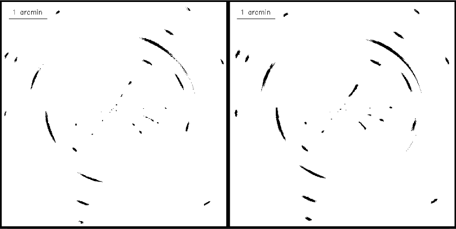
The third element are the lensed images () which are calculated from the first two elements ( and ). This is done through a simple ray-tracing procedure. For each position in the image, we calculate the deflection angle, , and then the corresponding source plane position,, according to the lens equation (equation 1). If the calculated coincides with one of the original sources, we assign to the lensed image the value (colour) of that source. Otherwise that point in the lensed image is left dark (value 0 ). We repeat the operation for all the pixels (s) to produce a complete image. Also, since the sources are small compared with our pixel size and to avoid missing some sources, we oversample our pixels by subdividing them and checking each pixel at different locations ( with and ) The original sources are plotted in figure 2 and the corresponding s in the left panel of figure 3.
4 Gridifying the mass distribution
4.1 The matrix
As laid out in section 2 the basis of our non-parametric reconstruction method is the assumption that the real mass can be well approximated by a pixelized mass distribution. The matrix is then the matrix which casts the mass vector into the vector of deflection angles
| (6) |
For convenience rather than taking the mass distribution in each cell to be constant we assume it follows a Gaussian distribution centred in the centre of the cell with some dispersion. This allows us to calculate analytically the lensing contribution from each mass cell, saving valuable computer time. We use a dispersion of where is the size of the cell, and we have confirmed with simulations that the lensed image generated with this choice agrees well with the true lensed image using a relatively small number of cells. The detailed structure of the matrix will be explained in appendix A.
4.2 Multi resolution mass-grid
Rather than taking a uniform grid, it is better to construct a dynamical- or multi-resolution grid. By sampling dense regions more heavily, it is possible to reduce drastically the number of cells needed to accurately reproduce the lensing properties of the cluster. In other words we choose an adaptive grid which samples the dense cluster centre better than the outer regions. Since we do not actually know the density profile of the cluster, this multi-resolution grid must be obtained through an iterative procedure. An example of this process can be found on the SLAP111see http://darwin.cfa.harvard.edu/SLAP/ (Strong Lensing Analysis Package) webpage.
Given a mass estimate (a first mass estimate can be obtained with a coarse regular grid), we split a given cell into four sub-cells if the mass in the cell exceeds some threshold value. The lower this threshold, the higher the number of divisions and consequently the higher the final number of cells. The obtained grid can then be used for the next mass estimate, and the process can be repeated as necessary. Typically the mass estimate will improve with each iterative step as this dynamical grid allows for the relevant regions of the cluster to become resolved.
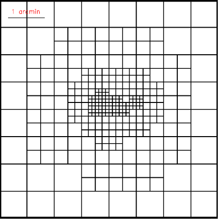
In figure 4 we show an example of a gridded version of the
true mass in figure 1 for a threshold of
h-1 M⊙.
This grid has 325 cells.
The corresponding (true) mass in the grid is shown in figure 5.
The parameter or equivalently the number of cells, , can be viewed
as a free parameter but also as a prior. Fixing it means we are fixing the minimum scale
or mass we are sensitive too. In a paralell paper (Diego et al. 2004) we explored
the role of and found that it can have a negative effect on the results
if it takes very large values. A natural upper limit for is 2 times the number of
pixels in the vector minus 2 times the number of sources (the factor 2 accounts
for the and positions). Our simulations show that a good election
for is normally of this upper limit.
For the shake of clarity it is useful to give some practical numbers. The image on the left of figure 3 has pixels from which 2156 pixels are part of one of the arcs so . These arcs are coming from 13 sources () and the lens plane is tipically divided in a few hundred cells ().
5 Inversion methods
In this section we will describe some inversion methods which can be applied to solve the problem. Most of these methods can be found in popular books like Numerical Recipes (Press et al. 1997). All these algorithms are being implemented in the package SLAP⋆ which will be made available soon.
Once we have the problem formulated in its linear form with all the unknowns on one side it is tempting to try a direct inversion of equation 5. Although the matrix is not square, one can find its inverse, , by decomposing into orthogonal matrices. This is similar to finding the eigenvalues and eigenvectors of . This approximation has its advantages as well as its drawbacks and we will explore this possibility later. However, we anticipate that degeneracies between neighboring pixels in the arcs as well as neighboring cells in the lens plane (not to mention the compact nature of the sources) will result in a system of linear equations which is not well behaved. The rank of the matrix will be normally smaller than its smaller dimension. Calculating the inverse in this situation is not a trivial task.
A second approach is rotating our system of linear equations using a transformation which is just . This transforms into a square, symmetric and positive definite matrix of dimension , which is better behaved than the original matrix.
However, the rank of is in generally smaller than its dimension and its inverse does not exist. The hope in this case must therefore be to find an approximate rather than exact solution to the system.
The third approach is the simplest and will be explored first. We assume we know nothing about the sources other than their redshift and that they are much smaller than the strong lensing arcs. This is the same as saying that the lens has to be such that it focuses the arcs into compact sources at the desired (known) redshift. This simple argument alone will turn out to be powerful enough to get a quick but good first estimate of the mass distribution in the lens plane.
We explore all these approaches below in reverse order.
5.1 A first approach: Minimizing dispersion in the source plane
In this subsection we will discuss the simplest (although effective) method to get a fast estimation of the mass using no prior information on the lens nor the sources. The problem then contains two sets of unknowns: The mass vector we want to determine, , and the positions of the sources. In general, for a finite number of observed arcs, there are several combinations of and which can reproduce the observations. The most obvious unphysical solution is the null solution, where the mass is zero and the sources identical to the observed arcs. The easiest way to avoid such unphysical solutions is to minimize the variance of the positions. This is equivalent to imposing that the vector really acts as a true lens: We require big arcs with large magnifications and multiple images separated by arcsec or even arc-min to focus into a rather compact region in the source plane. This minimization process assumes that we are able to associate the multiple lensed images with a particular source. This can be achieved with either spectroscopy or with morphology and the multicolor imaging of the arcs.
To minimize the variance in the source plane it is illustrative to follow the steepest descent path although other more effective minimization algorithms can be used (see below). Given an initial guess for the mass vector, one can calculate the derivative of the variance in the source plane as a function of the mass and minimize in the direction of the derivative. Once a minimum is found, we calculate the derivative in the new mass position and minimize again in an iterative procedure.
The quantity to be minimized is :
| (7) |
where the sum is over the number of identified sources and is the variance of the source in the source plane. That is;
| (8) |
where the ’s are calculated from equation 4 and the average is over the ’s corresponding to source . By combining equations 4 and 8 is easy to compute the derivative of with respect to .
| (9) |
where is the column of the matrix and the average is made only on the elements associated with the source . We should note that all equations involving the vectors , or have two components, and so there will be in fact two equations like equation 9. One for the component of and the other one for the component. At the end, the quantity we aim to minimize is . As we already mentioned, the minimization can be done following the path of steepest descent given by equation 9. This path will end in a minimum at the new mass . The process can be repeated by evaluating the new path at the new mass position until the variance is smaller than certain . A good choice for is to take a few times the expected variance for a population of galaxies at the measured redshifts. specific values for will be discussed later.
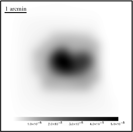
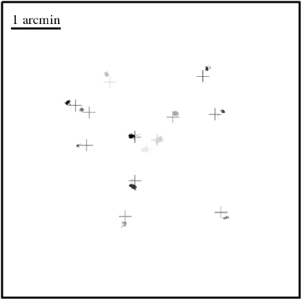
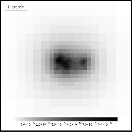
In practical terms the minimization is done through a series of iterations, gradually improving the dynamical grid as laid out in section 4.2. For each iteration the ability of the mass distribution to focus the s into compact sources is improved.
Equation 8 can be improved by weighting it with the amplification of the different images, assuming the errors in the image plane are similar from images to images. This point will not be explored here. The minimization of the variance is a powerful and robust method for finding a first guess for the mass vector without making assumptions about the sources. In fact, since the source positions can be estimated from equation 4, the minimization of the variance also provides us with an initial guess for these. The drawback is the slow convergence of the algorithm. A typical minimization may take several hours on a 1 GHz processor. In the next sub-section we will go a step further and we will include the positions in the minimization as well as speed up the convergence by orders of magnitude.
5.2 Biconjugate Gradient
Inversion of linear systems where the matrix dimensions are of order , is a numerically trivial problem for today’s computers provided the matrix is well behaved. If the matrix has null or negative eigenvalues, a direct inversion is not feasible and one has to aim to solve for some approximated solution. Our system of linear equations is a good example of an ill-conditioned one. Direct inversion of the matrix is not possible due to negative eigenvalues. However there is another important reason why we do not want to solve exactly (or invert) the system of equations. An exact solution means that we will recover a mass distribution which puts the arcs into delta function sources. As we will see later, this solution will be unphysical. Instead, we are interested in an approximated solution which does not solve exactly the system of equations and which has a residual. This residual will have the physical meaning of the extension of the sources or the difference between the point-like sources and the real, extended ones. The biconjugate gradient (Press et al. 1997) will be a useful way to regularize our problem.
The biconjugate gradient algorithm is one of the fastest and most powerful algorithms to solve for systems of linear equations. It is also extremely useful for finding approximate solutions for systems where no exact solutions exist or where the exact solution is not the one we are interested in. The latter will be our case. Given a system of linear equations;
| (10) |
a solution of this system can be found by minimizing the following function,
| (11) |
where is a constant. When the function is minimized, its gradient is zero.
| (12) |
That is, at the position of the minimum of the function we find the solution of equation (10). In most cases, finding the minimum of equation 11 is much easier than finding the solution of the system in 10 especially when no exact solution exists for 10 or does not have an inverse.
The biconjugate gradient finds the minimum of equation 11 (or equivalently, the solution of equation 10) by following an iterative process which minimizes the function in a series of steps no longer than the dimension of the problem. The beauty of the algorithm is that the successive minimizations are carried out on a series of orthogonal conjugate directions , , with respect to the metric . That is,
| (13) |
This condition is useful when minimizing in a multidimensional space since it guarantees that successive minimizations do not spoil the minimizations in previous steps.
Let us now turn to the system we want to solve, namely equation 5. The biconjugate gradient method assumes that the matrix ( matrix in equation 10) is square. For our case this does not hold since we typically have . Instead we build a new quantity, called the square of the residual,:
| (14) | |||||
| (15) |
By comparing equations 15 and 11 is easy to identify the terms, , and . Minimizing the quantity is equivalent to solving equation 5. To see this we only have to realize that
| (16) |
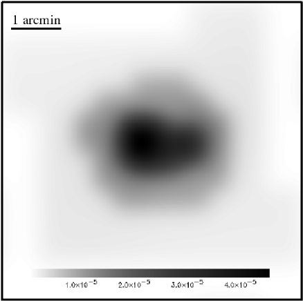
If an exact solution for equation 5 does not exist, the minimum of will give the better approximated solution to the system. The minimum can be now found easily with the biconjugate gradient (Press et al. 1997). For the case of symmetric matrices , the algorithm constructs two sequences of vectors and and two constants, and ;
| (17) |
| (18) |
| (19) |
| (20) |
At every iteration, an improved estimate of the solution is found by;
| (21) |
The algorithm starts with an initial guess for the solution, , and chooses the residual and search direction in the first iteration to be;
| (22) |
Note that is nothing but . Thus the algorithm chooses as a first minimization direction the gradient of the function to be minimized at the position of the first guess. Then it minimizes in directions which are conjugate to the previous ones until it reaches the minimum or the square of the residual is smaller than certain value .
The method has one potential pathological behavior when applied to our problem. One can not choose to be arbitrarily small. If one chooses a very small the algorithm will try to find a solution which focuses the arcs in sources which are delta functions. This is not surprising as we are assuming that all the unknown s are reduced to just s, i.e the point source solution (see figures 10 and 11 ) . The mass distribution which accomplishes this is usually very much biased compared to the right one. It shows a lot of substructure and it has large fluctuations in the lens plane. One therefore has to choose with a wise criteria. Since the algorithm will stop when we should choose to be an estimate of the expected dispersion of the sources at the specified redshifts. This is the only prior which has to be given to the method. However, we will see later how the specific value of is not very critical as long as it is within a factor of a few of the right source dispersion (see figure 18 below). Instead of defining in terms of is better to define it in terms of the residual of the conjugate gradient algorithm, . This will speed the minimization process significantly since we do not need to calculate the real dispersion at each step but to use the already estimated . Both residuals are connected by the relation,
| (23) |
Imposing a prior on the sizes of the sources means that we expect the residual of the lens equation, , to take typical values of the order of the expected dispersion of the sources at the measured redshifts. Hence we can define an of the form;
| (24) |
where the index runs from 1 to and is the dispersion (prior) assumed for the source associated to pixel and is a random number uniformly distributed over -1 and 1. Then, we can estimate as;
| (25) |
When calculating is is better to consider only the first columns of and discard the last . This is recommended to avoid that the 1s in this part of the matrix do not cancel out when multiplied by the random number and dominate the much smaller elements corresponding to the mass components. The last columns of should give 0 contribution when multiplied by the random vector. If we chose as a prior that the sources are Gaussians with a kpc located at the measured redshift, this renders . The reader will note that the chosen is a few times larger than the one we would assign to a typical galaxy. We will discuss this point later. The final result is shown in figures 8 and 9.
One has to be careful in not choosing the very small. In fact, they should be larger than the real dispersion of the source. Only when the number of grid points, , is large enough, can the gridded version of the true mass focus the arcs into sources which are similar in size to the real ones. If is not large enough, the gridded version of the true mass focuses the arcs into sources which are larger than the real sources. We should take this into account when fixing .
The reader can argue that a more clever way of including this prior information in the algorithm is by perturbing the elements in equation 5 (or similarly, equation 5 in Appendix A). This is done by adding some noise to the 1s in the two matrices in equation 37 (see Appendix A). One could for instance add Gaussian noise with a dispersion similar to the expected dispersion of the source at redshift . The reality however is that the quadratic nature of cancels out any symmetric perturbation added to the elements of . Thus, the result is similar if we perturb or not and we still have to include the prior and fix to be large enough so we do not recover the point source solution. This also tell us that this method is not very promising if one wants to include parity information in the recovery of the mass and sources. In the next subsection we will show a different approach which can include this parity information.
5.3 Singular Value Decomposition
The Singular Value Decomposition (hereafter SVD) algorithm allows for decomposition of a generic (with ) matrix into the product of 3 matrices, two orthogonal and one diagonal (e.g Press et al. 1997).
| (26) |
where is an orthogonal matrix, is an diagonal matrix whose elements in the diagonal are the singular values and is the transpose of an orthogonal matrix. When is symmetric, the SVD reduces to finding the eigenvectors and eigenvalues of A.
The advantage of this decomposition is that the inverse of is given by ;
| (27) |
where is another diagonal matrix whose elements are just the inverse of the elements of , that is . The proof follows from the property that and are orthogonal ().
In our case, we can use SVD to calculate the inverse of the matrix and find the solution, , directly by inverting equation (5)
| (28) |
Although the SVD allows us to invert the problem by calculating , its full power lies in its ability to solve a system approximately. The level of approximation can be controlled by setting a threshold in the matrix . In our problem, there will be many equations which are strongly correlated in the sense that most of the positions in a single arc will come from the same source (that is, they will have almost the same ). Also we have to keep in mind that we are using all the pixels in our data. This means that two equations corresponding to two neighboring pixels will look almost exactly the same. When one computes the SVD of the matrix , these two facts translate into a matrix with elements in the diagonal which are 0 or close to 0. The inverse of would be dominated by these small numbers and the solution will look very noisy. The good news about using SVD is that the most relevant information in the matrix is packed into the first few values (the largest values in ) while the small single values in will contain little information or the redundant information coming from neighboring pixels. One can just approximate by another matrix where all the elements in its diagonal smaller than certain threshold are set to 0. Also, in the inverse of , these elements are set to 0. The magic of this trick is that the solution found with this approximation will contain the main trend or main components of the mass distribution.
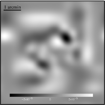
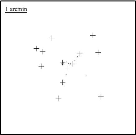
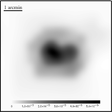
Another advantage of using the SVD algorithm is that in this case no prior on the extension of the sources is needed. The degree of accuracy is controlled by setting the threshold in the singular values of the matrix . Those elements in below the threshold are set to 0 and the same in its inverse. The threshold is usually set after looking at the singular values. The first ones will normally stay in some kind of plateau and after then the singular values will decrease rapidly. The threshold should be normally set immediately after the plateau. In figures 12 and 13 we show the result after decomposing in its SVD decomposition and calculating its inverse with (27).
Like the two previous algorithms, the SVD has its own pathologies. Using standard subroutines to find the SVD of usually return a no convergence error. This error comes from the nearly degenerate nature of . One has then to increase the number of maximum iterations on these subroutines or use a coarse version of where only a small fraction of the positions (or equivalently, rows) are considered. Another solution is inverting the preconditioned system of equations where we previously multiply for . This allows to use all the pixels and find the SVD of in a small number of iterations. However, using the SVD of instead of has a very interesting feature. It allows to introduce parity information in an effective way.
Contrary to the quadratic cases of minimization of the variance or the square of the residual , the SVD allows us to include parity information in the matrix which will not disappear when we look for the best solution. Since no or operations are involved, parity information will not cancel out. SVD could be an interesting way of fine tuning the solution by including the extra information coming from the parity of the arcs.
6 Incorporating the null space
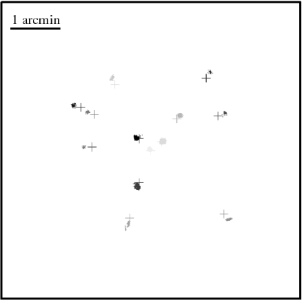
So far we have made use of the information contained in the observed strong lensing arcs. This gives us a solution which explains the data in the sense that it predicts arcs in the right positions but it could well happen that the solution over-predicts arcs. An example of this can bee seen by comparing the reproduced arcs in fig. (16) with the true arcs in fig. (3). Some of the reproduced arcs are slightly larger and span a larger area than the true ones, although the sources are perfectly reproduced in their true positions and the recovered mass is very close to the true mass distribution.
To avoid this we propose for the first time to include information from the null space, . That is, the part of the image which does not contain any arc. This space tell us where an arc should not appear but it does not tell us where the hypothetical should be. The only fair thing we can do is to impose that none of the pixels in the null space fall into the estimated of our solution. By achieving this we will have a solution which predicts the right arcs while not over-predicting arcs. The solution will be then fully consistent with the observed data.
The null space is connected to the solution X by;
| (29) |
It is evident that we want the new solution X ( and ) to be such that the new do not fall within a circle of radius centered in each one of the where is the prior with information on how extended are the sources. The null space will perturb the solution X in such a way that the new solution, is an approximated solution of equation 5 and satisfies all the constraints of the form .
The way we incorporate the constraints is by adopting an approach commonly used in penalized quadratic programming. We will minimize the new function
| (30) |
where the is a constant which guarantees that in the first iterations, the second term in equation 30 does not dominate the first and is a function which will penalize those models predicting falling near the positions which minimize . As a penalizing function we will choose an asymptotically divergent Gaussian
| (31) |
with,
| (32) |
Where is the x component of for the pixel in the null space. is our estimated value of (x component) and similarly for the y component. There are as many constraints of the form as there are pixels, , in the null space.
The parameter controls the degree of divergence of the Gaussian function. When we recover the classical Gaussian but as approaches 1 the Gaussian becomes more and more sharply without increasing its dispersion. For the Gaussian is infinite at (see figure 14. By minimizing the function with increasing values of we will find that in the limit the solution will push away those which originally were falling in the region defined by the set of .
Ideally we want to include all the dark or empty pixels in the space but this is, in general, found to be a waste of memory and computing time. The fact is that only the pixels which are hitting (or close to hit) one of the estimated positions of the sources will have some impact on the solution. Most of the pixels in the null space already satisfy all the constraints for the actual solution X. For this reason we will include only those for which the solution X predicts their corresponding are close to hitting (or actually hitting) a source. The space will include the observed ’s as a subspace. We have to exclude this subspace from before minimizing equation 30. This is, again, just an optimization process. In practice, one can include all the pixels in the image (excluding those containing part of an arc) in the null space.
After the minimization process is finished, the new solution will have the arcs falling in compact regions around while the extra-arcs produced by the previous solution will fall in regions outside areas around the .

¿From our simulation we have seen that addition of the null space induces small changes in the mass plane and it tends to stabilize the solution in the sense that it makes the recovered mass profile independent of the threshold . This is in fact an interesting bonus which comes with the addition of the null space. The new function to be minimized, , can be minimized until the true minimum is found. In this case, there is no equivalent of a point source solution. Since some of the are in fact very close to the observed , the solution which minimizes will focus those and in neighboring regions in the source plane. When minimizing there will be two competing effects. One will tend to increase the mass so it minimizes (point source solution). The other will tend to reduce the mass so the will be pushed away from the positions. The outcome will be a balanced situation between the trying to collapse into compact sources and the trying to escape the wells in the positions.
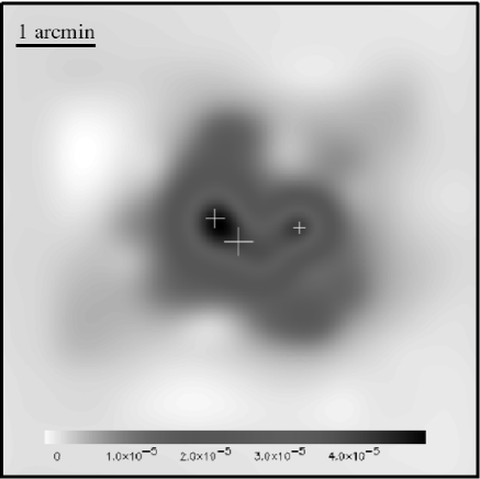
To accurately quantify the effect more simulations are needed. This will be done in a future paper but as an illustration we show in figure 15 the recovered mass after imposing the constraints in the space. The total mass is now only 1.2 % lower than the true mass. The new mass also contains more structure and starts showing the internal distribution of the main components of the cluster.
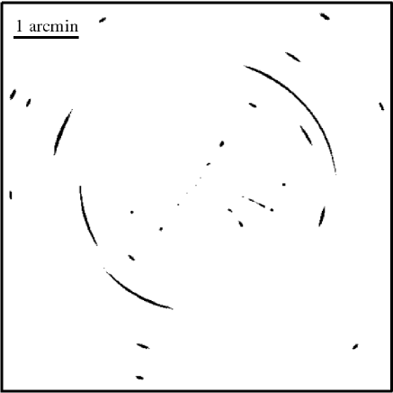
In figure 16 we show the predicted position for the arcs after combining the best mass together with the best estimate for the position of the sources. To compute the arcs we have assumed that each source is a circle with a radius kpc centred in the estimated best source positions and at the measured redshifts. By comparing figures 16 and figure 3 (left) we see that the predicted arcs matches very well the observed (simulated) data with the exception of some of the arcs near the center of the image.
7 Discussion
In this paper we have presented several approaches to non-parametric lens modelling. Using no information about luminosity distributions whatsoever, these methods perform remarkably well on simulated strong lensing data. One of the main conclusions of this work is simply that it works; It is possible to recover information about the mass distribution without using prior information on the same if one has a sufficiently large number of arcs. This can be seen in figure 17 where we show the recovered mass profiles compared with the original one. The recovered mass traces the real mass distribution up to furthest data point in the simulated image. Beyond this point, the recovered profile is insensitive to the data. When the minimization stops, the cells in the outer regions stay with a mass close to the one they had in the first step of the minimization. This point is discussed in more detail in Diego et al. (2004).
We are optimistic about the performance of these methods when used on future data, but we would also like to emphasize the potential pathologies. We will now discuss the major issues. As we have seen in section (2) the inversion algorithms rely on a linearization of the lens equation. We achieve that by decomposing the lens plane into small mass-cells and assuming that the gridded mass is a fair representation of the true underlying mass. This is true when the number of cells in the grid is large enough, but for a uniform grid this may mean using several thousand mass-cells, making the problem ill conditioned and underdetermined. By inverting the lens equation in a series of iterations we introduce an adaptive grid which optimizes the number of cells by sampling dense regions more heavily and using larger cells for underdense regions. This allows for good sampling of the lens without a huge number of cells.

However, the gridded mass plane is still an approximation to the true mass plane so we expect the solution to be an approximation to the true solution as well. Since a solution comprises not only the masses but the positions and extents of the sources as well, this means that we should expect these to also be approximations to the true ones. This has already been identified as one of the potential pathologies of the algorithm. Namely, if we try to focus the sources into very compact regions, with sizes comparable to the typical galaxy sizes at the relevant redshifts, the obtained mass is in general different to the true mass. In fact the best results are obtained when the mass plane focuses the arcs into regions which are a few times larger than the extent of the true sources. As we pointed out before, this reconstructed mass corresponds to a short-sighted version of the lens. This problem can be overcome by requiring the minimization algorithms stop once the recovered sources are a few times larger than the true sources. The extent of the true sources can be guessed from the redshift.

Introducing such a prior begs the question: How sensitive is the solution to the specific guess of prior? The answer is that it depends on exactly “how bad” that choice is. As long as we assume a source size significantly larger than the true sizes the actual solution does not change much and resembles well the true mass distribution. However, when trying to approach the true source size, the solutions changes rapidly away from the realistic model. The situation is shown in fig. (18). As shown in section 5.2 a given physical size corresponds to a given threshold, , and as long as this threshold is sufficiently large, , (corresponding to a physical size of kpc) the total mass is well behaved. If we instead demand that the physical size of the reconstructed sources be more realistic, say kpc, we get a threshold of for which the mass distribution is already starting to diverge away from the true mass. We therefore want the recovered sources to be larger than the true ones. In other words we want to recover a short-sighted cluster! In previous sections we have demonstrated non-parametric lens modelling using several different algorithms with promising results. However we have not yet addressed the question of uniqueness. Is there a unique solution, and if not, how different are the possible solutions?
The good news is that minimizing quadratic functions like the variance or the square of the residual guarantees that there is only one absolute minimum. This absolute minimum corresponds to the point source solution. The bad news is that this is not the solution we are looking for. As shown above, trying to focus the sources too much introduces artifacts in the mass distribution, so we need to stop the minimization at some step before the absolute minimum. In two dimensions it is easy to visualize that the quadratic function will have the shape of a valley, and stopping the minimization at some point before the actual minimum means choosing an ellipse on which all solutions are equally good. In many dimensions this is harder to visualize but we expect our obtainable solutions to lie on an N-dimensional ellipsoid around the minimum.
To get a quantitative grasp on how much these solutions differ in mass and source positions, we solve the equations for a range of random initial conditions. This is a manageable task since our minimization algorithm is extremely fast, taking only about second on a 1GHz processor. Also for speed purposes, we fix the grid to the one corresponding to the solution shown in figure 8. Fixing the grid speeds the process significantly since the matrix and the vector do not need to be recalculated in each minimization. In Diego et al. (2004) a similar process is followed carrying multiple minimizations but this time the grid is changed dynamically based on the solution found in the previous step. The authors found on that paper that the dispersion of the solutions increases due to the extra variability of the grid.
The result is shown in figure 19. The minimization process described in section 5.2 will stop at a different point in the N-dimensional ellipsoid for each set of different initial conditions. If the total mass of the initial mass distribution is very low the minimization will stop at solutions with mass below the true mass and positions further away from the center of the cluster than the real ones (dots). If instead we start with a total mass much larger than the true value, the minimization process returns higher masses and positions closer to the center of the potential (crosses). The situation improves when we impose that the total mass of the initial distribution have a reasonable value. In this case, the minimization stops in a region close to both the right mass and the right s. This argument motivates an iterative minimization where successive estimations for the mass are obtained at each step and used in the next.
Among the three algorithms presented in this work, the minimization of the variance is the less powerfull due to its low convergence. It is however interesting from a pedagogical point of view since it shows the existing degeneracies between the total mass of the cluster and the positions of the sources. The biconjugate gradient is orders of magnitude faster and is capable of finding the point source solution in a few seconds. The point source solution is however unphysical and a prior associated to the size of the sources is needed in order to stop the minimization process at the proper place. The good news are that the algorithm shows a weak sensitivity to this prior provided it is chosen with a minimum of wisdom. Since the point where the minimization stops depends on where the minimization starts, this also allows to study the range of possible models consistent with the data by minimizing many times while changing the initial conditions. This feature makes the biconjugate gradient very attractive for studying the space of solutions. This space can be reduced by including the extra-information contained in the null space, that is, the areas in the sky with no observed arcs. We have seen how this information can be naturally included in the minimization process by introducing a penalty function.
Finally, the SVD has the interesting feature that it allows to add extra information regarding the parity or resolved features in the arcs. This possibility has not been studied in detail in this paper but is definitely worth exploring since it would allow to recover smaller details in the mass distribution. The main drawbacks of the SVD is that the decomposition fails to converge when all the information is used and one has to use a coarse version of the data instead. The second drawback is that some of the singular values in the matrix are very small. These values will dominate the inverse if they are not masked by a threshold in the matrix . Choosing the value for this threshold is not very critical as long as its amplitude is large enough to mask the small singular values in .

The accuracy of the methods presented in this paper allow for high precision non-parametric mass reconstructions and direct mapping of the dark matter distribution of clusters. Previous works have suggested some discrepancy between mass estimates derived from different data (Wu & Fang 1997). Accuracy, combined with the speed of the algorithm opens the door to cosmological studies. Strong lensing analyses were predicted to yield interesting cosmological constraints, but due to the uncertainties in our understanding of galaxy clusters they have yet to live up to these predictions. A fast, per-cent level determination of cluster masses from lensing observations, could allow for sufficient statistical sampling to provide information about cosmological parameters. An interesting follow up to this work would be to establish what number of strong lensing systems, and what quality of data is necessary in order to make interesting constraints using our methods.
However the methods presented here should not be applied indiscriminately. For instance, if the reconstructed mass is systematically biased toward recovering less cuspy central regions this reduces the possibility of making conclusions about mechanisms for dark matter annihilation (Spergel & Steinhardt 2000, Wyithe et al. 2001, Boehm et al. 2004). If one is interested in using our methods to discuss this, that bias must be quantified. Due to lens resolution issues we anticipate that our reconstruction algorithms indeed have a bias in this direction and it is likely that other algorithms may suffer from similar problems. These and other poetential systematic errors shall be investigated in future works.
7.1 Future work
This paper is not intended to be an exhaustive exploration of the accuracy of non-parametric mass reconstruction methods but rather to help re-ignite debate and competition in the field, and demonstrate the feasibility and power of such methods in the face of new data. Specific issues such as magnitudes of the mass profile bias, source morphologies, surface brightness of the arcs, parity, projection effects as well as other relevant issues discussed above should be explored in order to improve the results. Special emphasis should be paid to the effects the grididification of the lens plane has on the results. An attempt to study this issue has been made on a second paper (Diego et al 2004) where the authors have shown that the grid may play an important role. In this paper we have presented the results using a very specific simulation. Although the algorithm has been tested with different simulations with positive results, it would be desirable to make a more detailed study of how the result is affected by issues like the structure of the lens, its symmetry or the number of sources and accuracy in their redshifts. Such a study would be even more interesting if a comparative study between parametric and non-parametric methods is done using the same simulations. Also interesting is to explore the effects of adding constraints in the mass of the type which may help to stabilize the solution even in the absence of a prior on the source sizes. This can be accomplished by adopting the techniques used in quadratic programming. All theses issues, although very interesting, are beyond the scope of this paper and will be studied in subsequent papers.
Although not discussed in this paper, a very interesting piece of work would be about the potentiality of an accurate strong lensing analysis as a cosmological tool (e.g Link & Pierce 1998, Yamamoto et al. 2001, Golse et al. 2002, Soucail et al. 2004). Previous works (Yamamoto et al. 2001, Chiba & Takahashi 2002, Sereno 2002, Dalal et al. 2004) suggest that the lensing observables are primarily dependent on the lens model while the dependency in the cosmological parameters is minor. Constraining the lens model with accuracy can open the window to do cosmology with strong lensing images. Is easy to imagine that a single image of a cluster with dozens of arcs coming from sources at different redshifts will constrain the lens model rather accurately and then, it will have something to say about the cosmology given the large number of distances involved in the analysis. All these issues are of great interest and they are intended to be studied in subsequent papers.
8 Acknowledgments
This work was supported by NSF CAREER grant AST-0134999, NASA grant NAG5-11099, the David and Lucile Packard Foundation and the Cottrell Foundation. The work was also partially supported by B. Jain through lousy poker playing. We thank D. Rusin and G. Bernstein for helpful discussions. We would like also to thank J.P Kneib for helpful suggestions.
References
- [1] Abdelsalam H.M., Saha P. & Williams, L.L.R., 1998, MNRAS, 294, 734.
- [2] Abdelsalam H.M, Saha P. & Williams, L.L.R., 1998, AJ, 116, 1541.
- [3] Bartelmann M., Narayan R., Seitz S. Schneider P., 1996, ApJ, 464, L115.
- [4] Beckwith S.V.W. et al. 2003, AAS, 202,1705
- [5] Blandford R.D., Narayan R. 1992, ARA&A, 30, 311.
- [6] Boehm C., Hooper D., Silk J., Casse M., Paul J., 2004, PhRvL, 92, 1301.
- [7] Brainerd T.G, Blandford R.D, Smail I, 1996, ApJ, 466, 623.
- [8] Bridle S.L, Hobson M.P., Lasenby A.N., Saunders R., 1998, MNRAS, 299, 895.
- [9] Broadhurst T.J., Taylor A.N., Peacock J.A., 1995, ApJ, 438, 49.
- [10] Broadhurst T.J., Huang X., Frye B., Ellis R., 2000, ApJL, 534, 15.
- [11] Broadhurst T.J. et.al. 2005, ApJ, 621, 53.
- [12] Chiba T., Takahashi R. 2002, Progress of Theoretical Physics, 107, 625.
- [13] Colley W.N., W.N, Tyson J.A., Turner E.L., 1996, ApJL, 461, 83.
- [14] Dahle H., Hannestad S.; Sommer-Larsen J. 2003, ApJ, 588, 73
- [15] Dalal N., Holder G., Hennawi, J.F. 2004, ApJ, 609, 50.
- [16] Diego J.M., Sandvik H.B., Protopapas P., Tegmark M., Benitez N., Broadhurst T., 2004, submitted to MNRAS, preprint astro-ph/0412191
- [17] Golse G., Kneib J.-P., Soucail G., 2002, A&A, 387, 788.
- [18] Guzik J., Seljak U., 2002, MNRAS, 335, 311.
- [19] Hudson M.J., Gwyn S.D.J., Dahle H., Kaiser N., 1998, ApJ, 503, 531.
- [20] Kaiser N. & Squires 1993, ApJ, 404, 441.
- [21] Kaiser N. 1995, ApJ, 439, L1.
- [22] Kneib J.-P., Mellier Y., Fort B., Mathez G., 1993,A&A, 273, 367.
- [23] Kneib J.-P., Mellier Y., Pello R., Miralda-Escudé J., Le Borgne J.-F.,Boehringer H., & Picat J.-P. 1995, A&A, 303, 27.
- [24] Kneib J.-P., Ellis R.S., Smail I.R., Couch W., & Sharples R. 1996, ApJ, 471, 643.
- [25] Kneib J.-P., 2002, The shapes of galaxies and their dark halos, Proceedings of the Yale Cosmology Workshop ”The Shapes of Galaxies and Their Dark Matter Halos”, New Haven, Connecticut, USA, 28-30 May 2001. Edited by Priyamvada Natarajan. Singapore: World Scientific, 2002, ISBN 9810248482, p.50
- [26] Kneib J.-P., Hudelot P., Ellis R.S., Treu T., Smith G.P., Marshall P., Czoske O., Smail I.R., Natarajan P., 2003, ApJ, 598, 804.
- [27] Kochanek C.S. & Blandford R.D., 1991, ApJ, 375, 492.
- [28] Link R. & Pierce M.J., 1998, ApJ, 502, 63.
- [29] Marshall P.J., Hobson M.P., Gull S.F., Bridle S.L, 2002, MNRAS, 335, 1037.
- [30] Meneghetti M., Jain B., Bartelmann M., Dolag K., 2004, astro-ph/0409030.
- [31] Narayan R. & Bartelmann M., Formation of Structure in the Universe, Proceedings of the 1995 Jerusalem Winter School. Edited by A. Dekel and J.P. Ostriker; Cambridge University Press 1999. p. 360.
- [32] Press W.H., Teukolsky S.A., Vetterling W.T., Flannery B.P., 1997, Numerical Recipes in Fortran 77. Cambrdige University Press.
- [33] Saha, P., Williams, L.L.R., 1997, MNRAS, 292, 148.
- [34] Saha P. 2000, AJ, 120, 1654.
- [35] Sand D.J., Treu T. Ellis R.S. 2002, ApJ, 574, 129.
- [36] Schneider P., Ehlers J., Falco E.E., 1993, Book Review: Gravitational lenses. Springer-Verlag, 1993.
- [37] Schneider P., 1995, A&A…302..639S.
- [38] Schneider P., & Seitz C. 1995, A&A, 294, 411.
- [39] Seitz C., & Schneider P. 1995, A&A, 297, 287.
- [40] Sereno M., 2002, A&A, 393, 757.
- [41] Soucail G., Kneib J.-P., Golse G. 2004, A&A, 417, L33.
- [42] Spergel D.N. & Steinhardt P.J., 2000, PhRvL, 84, 3760.
- [43] Taylor A.N., Dye S., Broadhurst T.J., Benitez N., van Kampen E. 1998, ApJ, 501, 539.
- [44] Tyson J.A., Kochanski G.P., Dell’Antonio I., 1998, ApJL, 498, 107.
- [45] Tegmark M., 2002, PhRvD, 66, 3507.
- [46] Trotter C.S., Winn J.N., Hewitt J. N., 2000, ApJ, 535, 671.
- [47] Wambsganss J., 1998, Living Reviews in Relativity, 1, 12.
- [48] Wyithe J.S.B., Turner E.L., Spergel D.N. 2001, ApJ, 555, 504.
- [49] Wu X.-P., & Fang L.-Z. 1997, ApJ, 483, 62.
- [50] Yamamoto K., & Futamase T., 2001, Progress of Theoretical Physics, 105, 5.
- [51] Yamamoto K., Kadoya Y., Murata T., Futamase T., 2001, Progress of Theoretical Physics, 106, 917.
APPENDIX A: THE AND MATRICIES
The matrix contains the information of how each mass element
affects the deflection angle. That is
| (33) |
Precisely how the matrix is constructed is a matter of convenience. Our specific choice is to put both and components of all the arc pixels into vectors with elements. The resulting is then a matrix.
In fact the structure of the matrix and the vectors are irrelevant as long as they combine to correctly represent the lens equation as
| (34) |
Each element in the matrix is computed as follows.
| (35) |
where
| (36) |
The index runs over the observed pixels,
index runs over the elements in the mass vector, .
The factor in equation (35) is just the difference
(in radians) between the x position in the arc (or x of pixel ) and
the x position of the cell in the mass grid
().
Similarly we can define and
. Also, for
we only have to change by .
Since we include the factor M⊙ in (see equation
36), the mass vector in equation 4
will be given in h-1 M⊙ units. The
dependency comes from the fact that in we have the ratio
which goes as .
Also we calculate and separately, the final
matrix entering in equation 4 contains both,
and (the same holds for the vectors and ).
One can rearrange the x and y components in any order.
The structure of the matrix is identical to the matrix but with the difference that it has additional columns (the location of the extra-columns is irrelevant as long as it is consistent with the location of the unknowns in the vector). Is easy to see that each one of these extra columns (with dimension ) corresponds to one of the sources. Since the matrix has to contain both the x and y component, the first/second half of each one of the extra columns will be all 0’s depending on if it corresponds to the y/x component of . The other half will be full of 0’s and 1’s, the 1’s being in the positions associated with that particular source, the 0’s elsewhere. That is, the lens equation can be written explicitly as ( denotes matrix and denotes vector);
| (37) |
Where again, and are two dimensional vectors containing the x and y positions, respectively, of the pixels in the observed arcs. The two ( matrices and contain the x and y lensing effect of the cell on the pixel . The dimensional matrices and are full of 0’s (the matrix) or contain 1’s (the matrix) in the positions () where the th pixel comes from the source () and 0 elsewhere. The vector contains the gridded masses we want to estimate. contains the central x positions of the sources. Similarly, will contain the central y positions.