THE LARGE-SCALE STRUCTURE OF THE UNIVERSE
IN ONE DIMENSION

Abstract

I investigate statistical properties of one-dimensional fields in the universe such as the Ly$\alpha$ forest (Ly$\alpha$ absorptions in the quasar spectrum) and inverted line-of-sight densities. The Ly$\alpha$ forest has opened a great window for studying the large-scale structure of the universe, because it can probe the cosmic density field over a wide range of redshift at relatively high resolution, which has not been easily accessible with other types of observations.

The power spectrum completely characterizes Gaussian random fields. However, because of gravitational clustering, the cosmic density field is already quite non-Gaussian on scales below 10 $h^{-1}$Mpc at redshift $z=3$. I analyze the covariance of the one-dimensional mass power spectrum, which involves a fourth-order statistic, the trispectrum. The covariance indicates that Fourier modes in the cosmic density field are highly correlated and that the variance of the measured one-dimensional mass power spectrum is much higher than the expectation for Gaussian random fields. It is found that rare high-density structures contribute significantly to the covariance. The window function due to the length of lines of sight introduces additional correlations between different Fourier modes.

In practice, one observes quasar spectra instead of one-dimensional density fields. As such, flux power spectrum has been the basis of many works. I show that the nonlinear transform between density and flux quenches the fluctuations so that the flux power spectrum is less sensitive to cosmological parameters than the one-dimensional mass power spectrum. The covariance of the flux power spectrum is nearly Gaussian, which suggests that higher-order statistics may be less effective for the flux.

Finally, I provide a method for inverting Ly$\alpha$ forests and obtaining line-of-sight densities, so that statistics can be measured from one-dimensional density fields directly.

STATEMENT BY AUTHOR

This dissertation has been submitted in partial fulfillment of requirements for an advanced degree at The University of Arizona and is deposited in the University Library to be made available to borrowers under rules of the Library.

Brief quotations from this dissertation are allowable without special permission, provided that accurate acknowledgment of source is made. Requests for permission for extended quotation from or reproduction of this manuscript in whole or in part may be granted by the copyright holder.

SIGNED:

ACKNOWLEDGMENTS

I thank my advisors David Burstein, Daniel Eisenstein, and Li-Zhi Fang for their supervision and guidance over the course of my study.

I also thank my mentors and collaborators, Bruce Barrett, Romeel Davé, Xiaohui Fan, Priya Jamkhedkar, Fulvio Melia, Petr Navrátil, Andreas Nogga, Michael Shupe, James Vary, Rogier Windhorst, and Ann Zabludoff. Without them, I would probably have spent a lot more time practicing trial and error.

I appreciate the financial support from Bruce in the Spring and Summer of 2003, during which ideas in this dissertation germinated. I have benefited from grants from the Theoretical Astrophysics Program and registration fee waivers from the Physics Department.

I am grateful to my wife, Yue, for her enduring support.

DEDICATION

This dissertation is dedicated to my parents, Hua’an and Lanzhen, and my wife, Yue.

TABLE OF CONTENTS

toc

LIST OF FIGURES

lof

LIST OF TABLES

lot

LIST OF ABBREVIATIONS

2dF	Two Degree Field (Survey)
CDM	Cold Dark Matter
CMB	Cosmic Microwave Background
EOS	Equation of State
GRF	Gaussian Random Field
IGM	Intergalactic Medium
LCDM	$\Lambda$ CDM (Model) or Low-Density-and-Flat CDM (Model)
LOS	Line of Sight or Line-of-Sight
OCDM	Open CDM (Model)
PS	Power Spectrum
QSO	Quasi-Stellar Object or Quasar
SCDM	Standard CDM (Model)
SDSS	Sloan Digital Sky Survey
SPH	Smooth-Particle Hydrodynamics
TCDM	$\tau$ CDM (Model) or Tilted CDM (Model)
TSC	Triangular-Shaped Cloud (Assignment Function)
UV	Ultraviolet
WHIM	Warm-Hot Intergalactic Medium
WMAP	Wilkinson Microwave Anisotropy Probe

Chapter 1 Introduction

The cosmological principle, i.e. the assumption of homogeneity and isotropy (Milne 1935), has been born out by decades of tests (for reviews, see Peebles 1980, 1993). As profound as it is, structures do rise from minute primordial fluctuations because of gravitational instability (e.g. Jeans 1928; Lemaître 1934). On scales beyond galaxy clusters, the cosmic density field remains in the linear or quasi-linear regime, which means the formation and evolution of the large-scale structure still bears the initial imprint of cosmology. In other words, the large-scale structure is a sensitive tool for measuring fundamental properties of the universe.

Galaxies and clusters of galaxies were the first objects used to study the large-scale structure of the universe (e.g. Hubble 1934; Shapley 1934). Recent surveys include the Center for Astrophysics Survey (Huchra et al. 1990), the Automatic Plate-measuring Machine Survey (Maddox et al. 1990), the Las Campanas Redshift Survey (Shectman et al. 1996), the Infrared Astronomical Satellite Point Source Catalog Redshift Survey (Saunders et al. 2000), the Two Degree Field (2dF) Galaxy Redshift Survey (Colless et al. 2001), and the Sloan Digital Sky Survey (SDSS, initial release, Stoughton et al. 2002). One useful statistic is the galaxy clustering power spectrum (PS, Peacock 1991; Baugh & Efstathiou 1993; Fisher et al. 1993; Lin et al. 1996; Percival et al. 2001; Dodelson et al. 2002). Because galaxies reside in high-density peaks of the cosmic density field, galaxy statistics may be (slightly) biased with respect to the true statistics of the field (Dekel & Silk 1986; Gaztanaga & Frieman 1994; Kauffmann, Nusser & Steinmetz 1997; Dekel & Lahav 1999; Benson et al. 2000; Peacock & Smith 2000; Somerville et al. 2001; Verde et al. 2002; Weinberg et al. 2004). Galaxy surveys are often limited by depth. For example, the mean redshift of the above-mentioned surveys is around 0.1 or less, which translates to a volume on the order of a thousandth of the Hubble volume. Such a small survey volume limits our ability to study the large-scale structure at high redshift and its evolution.

Quasars, or quasi-stellar objects (QSOs), are far more luminous than galaxies, and they have been observed near the edge of the visible universe (Fan et al. 2001, 2003). The 2dF QSO survey (Boyle et al. 2000) and the SDSS will provide large QSO samples for statistics such as the QSO clustering correlation function and PS (Shaver 1984; Shanks et al. 1987; Iovino & Shaver 1988; Mo & Fang 1993; Shanks & Boyle 1994; La Franca, Andreani & Cristiani 1998; Outram et al. 2003). Like galaxies, QSOs also live in high-density peaks of the universe, and their statistics may be biased as well. In fact, galaxies are often found to cluster around QSOs (Tyson 1986; Fisher et al. 1996; Pascarelle et al. 2001; Kauffmann & Haehnelt 2002). Because of large separations, QSOs statistics are more reliable for studying the clustering of matter above 10 $h^{-1}$Mpc, where $h$ is the Hubble constant in units of 100 km s^-1 Mpc^-1.

One often sees numerous Ly$\alpha$ absorption lines in QSO spectra that are resulted from absorptions by the diffusely distributed and photoionized intergalactic medium (IGM). Absorption systems that have neutral-hydrogen column density $10^{12}\leq N_{\rm HI}\leq 10^{17}$ cm^-2 are also called the Ly$\alpha$ forest (for a review, see Rauch 1998). It has been demonstrated by various hydrodynamical simulations that the IGM traces the density of the underlying mass field on large scales (Cen et al. 1994; Zhang, Anninos & Norman 1995; Hernquist et al. 1996; Miralda-Escudé et al. 1996; Davé et al. 1997; Bryan et al. 1999). In other words, baryon densities in Ly$\alpha$ absorption systems are roughly proportional to total matter densities for $\rho/\bar{\rho}\lesssim 10$ (Bi & Davidsen 1997; Gnedin & Hui 1998; Zhang et al. 1998), where $\rho$ is the density and $\bar{\rho}$ is the mean density. Therefore, the Ly$\alpha$ forest offers a less biased probe of the large-scale structure of the universe.

The Ly$\alpha$ forest has been observed up to $z\sim 6$ (Becker et al. 2001), beyond which neutral hydrogen (H i) completely absorbs the QSO flux at rest wavelength $\lambda_{0}=1216$ Å due to the Gunn-Peterson effect (Gunn & Peterson 1965). For each line of sight (LOS) to a QSO, one can sample the density field almost continuously in one dimension and obtain more information than the clustering of QSOs. With enough LOS’s covering $0\leq z\lesssim 6$, the Ly$\alpha$ forest will enable us to establish a more complete picture of the universe and its evolution. In fact, statistics of the Ly$\alpha$ forest have been applied to many aspects of large-scale structure studies such as recovering the initial linear mass PS (Croft et al. 1998, 1999; Hui 1999; Feng & Fang 2000; McDonald et al. 2000; Gnedin & Hamilton 2002; Zaldarriaga, Scoccimarro & Hui 2003), measuring the flux PS and bispectrum (Hui et al. 2001; Mandelbaum et al. 2003; Kim et al. 2004; Viel et al. 2004), estimating cosmological parameters (McDonald & Miralda-Escudé 1999; Zaldarriaga, Hui & Tegmark 2001; Croft et al. 2002; Seljak, McDonald & Makarov 2003; McDonald 2003; Viel et al. 2003), inverting the Ly$\alpha$ forest (Nusser & Haehnelt 1999; Pichon et al. 2001; Zhan 2003), finding the applicable range of the hierarchical clustering model (Feng, Pando & Fang 2001; Zhan, Jamkhedkar & Fang 2001), and estimating the velocity field (Zhan & Fang 2002). These studies show that the Ly$\alpha$ forest has provided an important complement to studies based on galaxy and QSO samples.

The unique nature of the Ly$\alpha$ forest brings its own subtleties. First, the Ly$\alpha$ forest probes well into the nonlinear regime, e.g. from several $h^{-1}$Mpc down to tens of $h^{-1}$kpc. The non-Gaussianity on such small scales plays an important role in statistics, and cosmological hydrodynamical simulations are needed for the study. Second, the direct observable is the Ly$\alpha$ flux rather than the density. Statistics of the density, which are more fundamental to cosmology, have to be recovered from flux statistics. Third, the observed Ly$\alpha$ forest may be affected by many elements such as the continuum fitting (Hui et al. 2001), the UV ionization background (Rauch et al. 1997; Scott et al. 2000; McDonald & Miralda-Escudé 2001; Meiksin & White 2004), saturated Ly$\alpha$ absorptions (Zhan 2003; Viel et al. 2004), metal-line contaminations, and redshift distortion. At low redshift, additional uncertainties arise from the thinning of the Ly$\alpha$ forest (Riediger, Petitjean & Mücket 1998; Theuns, Leonard & Efstathiou 1998) and the shock-heated warm-hot IGM (WHIM, Davé et al. 1999; Davé & Tripp 2001; Davé et al. 2001).

This dissertation focuses on theoretical and numerical aspects of one-dimensional statistics of the large-scale structure. It is organized as follows. Chapter 2 discusses the relation between the one-dimensional PS and the three-dimensional PS with an emphasis on spatial average. The covariance of the one-dimensional mass PS is derived for Gaussian random fields (GRFs) and the cosmic density field in Chapter 3. One-dimensional mass PS’s and their covariances are calculated in Chapter 4 for simulated density fields. Flux PS’s and their covariances are measured from simulated as well as observed Ly$\alpha$ forests in Chapter 5, and they are compared with corresponding mass PS’s and covariances. Effects of the UV ionization background and the WHIM are also discussed there. Chapter 6 introduces the mean density–width relation (Zhan 2003) and its application in extracting density information from saturated Ly$\alpha$ absorptions. Chapter 7 concludes the dissertation.

Chapter 2 One-Dimensional Power Spectrum

The one-dimensional mass PS and its relation to the three-dimensional mass PS have been frequently utilized to recover the linear mass PS from the Ly$\alpha$ forest (Croft et al. 1998, 1999, 2002; Gnedin & Hamilton 2002). This opens a great window for studying the large-scale structure of the universe over a wide range of redshift.

For an ensemble of isotropic fields, the one-dimensional mass PS $P_{\rm 1D}(k)$ is a simple integral of the three-dimensional mass PS $P(k)$ (Lumsden, Heavens & Peacock 1989),

$$P_{\rm 1D}(k)=\frac{1}{2\pi}\int_{k}^{\infty}P(k^{\prime})k^{\prime}\,{\rm d}k^{\prime},$$ (2.1)

where $k$ is the LOS wavenumber. However, there is only one observable universe. The ensemble average has to be replaced by a spatial average. For instance, one may sample multiple LOS densities from the three-dimensional cosmic density field and use the average PS of the one-dimensional densities in place of the ensemble-average quantity. Such spatial average alters the relation between the one-dimensional mass PS and the three-dimensional mass PS. I discuss the modification to equation (2.1) and its significance in this chapter. Although I use the density field as an example, the results obtained here are generic.

2.1 Three-Dimensional Power Spectrum

It is beneficial to review the three-dimensional PS before we look at the one-dimensional PS. I assume the following convention of Fourier transforms for a cubic density field $\rho({\bf x})$ in the volume $V=B^{3}$:

$$\delta({\bf x}) = \frac{1}{V}\sum_{{\bf n}=-\infty}^{\infty}\hat{\delta}({\bf n})\,e^{2\pi i{\bf n}\cdot{\bf x}/B},$$ (2.2)

$$\hat{\delta}({\bf n}) = \int_{V}\delta({\bf x})\,e^{-2\pi i{\bf n}\cdot{\bf x}/B}\,{\rm d}{\bf x},$$

where $\delta({\bf x})=[\rho({\bf x})-\bar{\rho}]/\bar{\rho}$ is the overdensity, $\hat{\delta}({\bf n})$ is the Fourier transform of $\delta({\bf x})$, the summation $\sum_{{\bf n}=-\infty}^{\infty}$ is an abbreviation for $\sum_{n_{1},n_{2},n_{3}=-\infty}^{\infty}$, and the wavevector ${\bf k}$ equals $2\pi{\bf n}/B$ with integral $n_{1}$, $n_{2}$, and $n_{3}$. I choose this form of Fourier transforms because real surveys always have a finite volume and, after all, the visible universe is finite. Equation (2.2) will approach the limit of continuous Fourier transforms as the volume increases.

With the understanding that Fourier modes exist only at discrete wavenumbers, i.e. $n_{1}$, $n_{2}$, and $n_{3}$ are integers, one may use ${\bf k}$ and ${\bf n}$ interchangeably for convenience. To be complete, the orthonormality relations are

$$\frac{1}{V}\int_{V}e^{-2\pi i({\bf n}-{\bf n}^{\prime})\cdot{\bf x}/B}{\rm d}{\bf x} = \delta^{\rm K}_{{\bf n},{\bf n}^{\prime}},$$ (2.3)

$$\frac{1}{V}\sum_{{\bf n}=-\infty}^{\infty}e^{2\pi i{\bf n}\cdot({\bf x}-{\bf x}^{\prime})/B} = \delta^{\rm D}({\bf x}-{\bf x}^{\prime}),$$ (2.4)

where $\delta^{\rm K}_{{\bf n},{\bf n}^{\prime}}$ is the three-dimensional Kronecker delta function, and $\delta^{\rm D}({\bf x}-{\bf x}^{\prime})$ the Dirac delta function.

The three-dimensional mass PS of the universe is defined through

$$\langle\hat{\delta}({\bf k})\hat{\delta}^{*}({\bf k}^{\prime})\rangle=P({\bf k})V\delta^{\rm K}_{{\bf n},{\bf n}^{\prime}},$$ (2.5)

where $\langle\ldots\rangle$ stands for an ensemble average. One may define an observed PS,

$$P^{\prime}({\bf k})=|\hat{\delta}({\bf k})|^{2}/V,$$ (2.6)

so that $P({\bf k})=\langle P^{\prime}({\bf k})\rangle$. For an isotropic field, $P({\bf k})$ is a function of the length of ${\bf k}$ only, i.e. $P({\bf k})\equiv P(k)$. A shot-noise term should be included if the PS is measured from discrete objects, and it is inversely proportional to the mean number density of the objects. I neglect the shot-noise in this dissertation. An alternative definition of $P(k)$ utilizes the correlation function $\xi(r)$, e.g.

$$\xi(r) = \langle\delta({\bf x}+{\bf r})\delta({\bf x})\rangle,$$ (2.7)

$$P(k) = \int_{V}\xi(r)\,e^{-i{\bf k}\cdot{\bf r}}\,{\rm d}{\bf r}.$$ (2.8)

The four-point function of $\delta({\bf x})$ is

$$\langle\delta({\bf x}_{\rm a})\delta({\bf x}_{\rm b})\delta({\bf x}_{\rm c})\delta({\bf x}_{\rm d})\rangle=\xi_{\rm ab}\xi_{\rm cd}+\xi_{\rm ac}\xi_{\rm bd}+\xi_{\rm ad}\xi_{\rm bc}+\eta,$$ (2.9)

where $\xi_{\rm ab}$ stands for $\xi(|{\bf x}_{\rm a}-{\bf x}_{\rm b}|)$, and $\eta$ is the reduced four-point correlation function that has six degrees of freedom arising from relative coordinates of the four points under the constraint of homogeneity (Peebles 1980). From equations (2.8) and (2.9), we have the four-point function of $\hat{\delta}({\bf k})$

$$\langle\hat{\delta}({\bf k}_{\rm a})\hat{\delta}^{*}({\bf k}_{\rm b})\hat{\delta}({\bf k}_{\rm c})\hat{\delta}^{*}({\bf k}_{\rm d})\rangle = V^{2}\big{[}P(k_{\rm a})P(k_{\rm c})\delta^{\rm K}_{{\bf n}_{\rm a},{\bf n}_{\rm b}}\delta^{\rm K}_{{\bf n}_{\rm c},{\bf n}_{\rm d}}+P(k_{\rm a})P(k_{\rm b})\delta^{\rm K}_{{\bf n}_{\rm a},{\bf n}_{\rm d}}\delta^{\rm K}_{{\bf n}_{\rm b},{\bf n}_{\rm c}}\big{]}$$ (2.10)

$$+VT({\bf k}_{\rm a},-{\bf k}_{\rm b},{\bf k}_{\rm c},-{\bf k}_{\rm d}),$$

where

$$T({\bf k}_{\rm a},{\bf k}_{\rm b},{\bf k}_{\rm c},{\bf k}_{\rm d})=\frac{1}{V}\int_{V}\eta\,\exp[{-i{\bf k}_{\rm a}\cdot{\bf x}_{\rm a}-i{\bf k}_{\rm b}\cdot{\bf x}_{\rm b}-i{\bf k}_{\rm c}\cdot{\bf x}_{\rm c}-i{\bf k}_{\rm d}\cdot{\bf x}_{\rm d}}]\,{\rm d}{\bf x}_{\rm a}\,{\rm d}{\bf x}_{\rm b}\,{\rm d}{\bf x}_{\rm c}\,{\rm d}{\bf x}_{\rm d}$$

is the trispectrum, and the wavevectors are restricted to be in the same hemisphere so that the term $P(k_{\rm a})P(k_{\rm b})\delta^{\rm K}_{{\bf n}_{\rm a},-{\bf n}_{\rm c}}\delta^{\rm K}_{{\bf n}_{\rm b},-{\bf n}_{\rm d}}$ does not appear. Since the reduced four-point correlation function $\eta$ is a six-variable function, there is a redundancy in the variables of the trispectrum. It is evident from the four-point function that the covariance of the three-dimensional mass PS is (see also Meiksin & White 1999; Cooray & Hu 2001)

$$\sigma^{2}({\bf k},{\bf k}^{\prime}) = \langle[P^{\prime}({\bf k})-P({\bf k})][P^{\prime}({\bf k}^{\prime})-P({\bf k}^{\prime})]\rangle=\langle\hat{\delta}({\bf k})\hat{\delta}^{*}({\bf k})\hat{\delta}({\bf k}^{\prime})\hat{\delta}^{*}({\bf k}^{\prime})\rangle V^{-2}-P(k)P(k^{\prime})$$ (2.11)

$$= P^{2}(k)\delta^{\rm K}_{{\bf n},{\bf n}^{\prime}}+V^{-1}T({\bf k},-{\bf k},{\bf k}^{\prime},-{\bf k}^{\prime}).$$

For GRFs, the trispectrum vanishes, and

$$\sigma^{2}({\bf k},{\bf k^{\prime}})=P^{2}(k)\delta^{\rm K}_{{\bf n},{\bf n}^{\prime}}.$$ (2.12)

Since the survey volume is always smaller than the observable universe, the covariance will be modified according to Feldman, Kaiser & Peacock (1994), and the non-Gaussianity will further alter the covariance through the trispectrum.

2.2 One-Dimensional Power Spectrum

For a LOS density that is along the $x_{3}$-axis and sampled at $(x_{1},x_{2})$, the one-dimensional Fourier transform gives

$$\tilde{\delta}({\bf x}_{\perp},n_{3})=\int_{0}^{B}\delta({\bf x})\,e^{-2\pi in_{3}x_{3}/B}\,{\rm d}x_{3}=\frac{1}{B^{2}}\sum_{{\bf n}_{\perp}=-\infty}^{\infty}\hat{\delta}({\bf n}_{\perp},n_{3})\,e^{2\pi i{\bf n}_{\perp}\cdot{\bf x}_{\perp}/B},$$ (2.13)

where the subscript $\perp$ signifies the first two components of a vector, i.e. ${\bf x}_{\perp}=(x_{1},x_{2})$. Similar to the three-dimensional mass PS, the one-dimensional mass PS is expected to follow

$$\langle\tilde{\delta}({\bf x}_{\perp},n_{3})\tilde{\delta}^{*}({\bf x}_{\perp},n^{\prime}_{3})\rangle=P_{\rm 1D}(n_{3})B\delta^{\rm K}_{n_{3},n^{\prime}_{3}}.$$ (2.14)

Substituting equation (2.13) in equation (2.14) and making use of equation (2.5), one finds the relation between the one-dimensional mass PS and the three-dimensional mass PS,

$$P_{\rm 1D}(n_{3})=\frac{1}{B^{2}}\sum_{{\bf n}_{\perp}=-\infty}^{\infty}P({\bf n}_{\perp},n_{3}),$$ (2.15)

which is a discrete analog of equation (2.1).

Practically, one measures PS’s of LOS densities sampled at some locations, e.g.

$$P^{\prime}_{\rm 1D}({\bf x}_{\perp},k_{3})=|\tilde{\delta}({\bf x}_{\perp},k_{3})|^{2}/B.$$ (2.16)

A simple estimator of the one-dimensional mass PS may be constructed by a spatial average over many LOS’s, i.e.

$$P^{\prime}_{\rm 1D}(k_{3})=\langle P^{\prime}_{\rm 1D}({\bf x}_{\perp},k_{3})\rangle_{{\bf x}_{\perp}},$$ (2.17)

where $\langle\ldots\rangle_{{\bf x}_{\perp}}$ stands for a spatial average over all LOS’s in the sample. To assess the performance of the estimator, two questions need to be addressed: (1) How does $P^{\prime}_{\rm 1D}(k_{3})$ relate itself to $P^{\prime}({\bf k})$; and (2) What is the covariance of $P^{\prime}_{\rm 1D}(k_{3})$ with respect to $P_{\rm 1D}(k_{3})$? The rest of this chapter answers the former, and Chapter 3 the latter.

For simplicity, I assume that LOS’s are sampled regularly in transverse directions at an interval of $b=B/m$, where $m$ is an integer. Each LOS has a length of $B$, and ${\bf x}_{\perp}=b{\bf l}_{\perp}$ with $l_{1},l_{2}=0,\ldots,m-1$. The estimated one-dimensional mass PS is then

$$P^{\prime}_{\rm 1D}(n_{3}) = \frac{1}{m^{2}}\sum_{{\bf l}_{\perp}=0}^{m-1}|\tilde{\delta}(b{\bf l}_{\perp},n_{3})|^{2}/B$$ (2.18)

$$= \frac{1}{m^{2}B^{5}}\sum_{{\bf l}_{\perp}=0}^{m-1}\Big{|}\sum_{{\bf n}_{\perp}=-\infty}^{\infty}\hat{\delta}({\bf n}_{\perp},n_{3})\,e^{2\pi i{\bf n}_{\perp}\cdot{\bf l}_{\perp}/m}\Big{|}^{2}$$

$$= \frac{1}{B^{5}}\sum_{{\bf n}_{\perp},\,{\bf j}_{\perp}=-\infty}^{\infty}\hat{\delta}({\bf n}_{\perp},n_{3})\,\hat{\delta}^{*}({\bf n}_{\perp}\!+m{\bf j}_{\perp},n_{3}),$$

where the equality,

$$\frac{1}{m}\sum_{l=0}^{m-1}e^{2\pi i(n-n^{\prime})l/m}=\delta^{\rm K}_{n,n^{\prime}+mj}\quad j=0,\pm 1,\ldots,\pm\infty,$$ (2.19)

has been used to obtain the last line of equation (2.18). It is easy to show with equation (2.18) that

$$P_{\rm 1D}(k_{3})=\langle P_{\rm 1D}^{\prime}(k_{3})\rangle=\langle P_{\rm 1D}^{\prime}({\bf x}_{\perp},k_{3})\rangle.$$ (2.20)

Note that there is no spatial average on the far right side of equation (2.20). It seems that only in the limit $m\to\infty$ do $P^{\prime}_{\rm 1D}(k_{3})$ and $P^{\prime}({\bf k})$ follow the same relation as equations (2.1) and (2.15), i.e. $P^{\prime}_{\rm 1D}(k_{3})=\sum_{{\bf n}_{\perp}=-\infty}^{\infty}P^{\prime}({\bf k}_{\perp},k_{3})/B^{2}$, where I have assumed $\hat{\delta}(\infty)=0$ so that only ${\bf j}_{\perp}=(0,0)$ terms contribute. In other words, one would need a high sampling rate in the transverse direction to accurately recover $P^{\prime}({\bf k})$ from $P^{\prime}_{\rm 1D}(k_{3})$ regardless the scale of interest. This apparently contradicts the new sampling paradigm (Unser 2000), according to which one only has to prefilter signals and sample them at a minimum rate of twice the frequency (wavenumber) of interest. However, the one-dimensional mass PS is a projection of the three-dimensional mass PS, so that even a prefiltering of transverse modes on small scales will lead to a distortion of the measured one-dimensional mass PS on large scales.

2.3 Aliasing

Without losing generality, one may choose $m$ to be even, so that equation (2.18) can be re-arranged as

$$P^{\prime}_{\rm 1D}(n_{3}) = \frac{1}{B^{2}}\sum_{{\bf n}_{\perp}=-m/2}^{m/2}P_{\rm a}({\bf n}_{\perp},n_{3})$$

$$= \frac{1}{B^{2}}\sum_{{\bf n}_{\perp}=-\infty}^{\infty}P^{\prime}({\bf n}_{\perp},n_{3})+A(n_{3}),$$

where

$$P_{\rm a}({\bf n}_{\perp},n_{3})=\frac{1}{V}\Big{|}\sum_{{\bf j}_{\perp}=-\infty}^{\infty}\hat{\delta}({\bf n}_{\perp}\!+m{\bf j}_{\perp},n_{3})\Big{|}^{2},$$ (2.22)

and

$$A(n_{3})=\frac{1}{B^{5}}\sum_{\mbox{\scriptsize$\begin{array}[]{c}{\bf j}_{\perp},{\bf j}^{\prime}_{\perp}\!=-\infty\\ {\bf j}^{\prime}_{\perp}\!\neq 0\end{array}$}}^{\infty}\sum_{{\bf n}_{\perp}\!=-m/2}^{m/2}\hat{\delta}({\bf n}_{\perp}\!+m{\bf j}_{\perp},n_{3})\,\hat{\delta}^{*}({\bf n}_{\perp}\!+m{\bf j}_{\perp}\!+m{\bf j}^{\prime}_{\perp},n_{3}).$$ (2.23)

Equation (2.3) provides two equivalent views of the sampling effect. On one hand, the one-dimensional mass PS is a sum of the aliased three-dimensional mass PS, $P_{\rm a}({\bf k})$, that is sampled by a grid of $m\times m$ LOS’s. On the other hand, it is a complete sum of the underlying three-dimensional mass PS with an extra term $A(k_{3})$ that is determined by the sampling rate and properties of the density field.

The discrete Fourier transform cannot distinguish a principal mode at $|k|\leq k_{\rm Nyq}$ from its aliases at $k\pm 2k_{\rm Nyq},k\pm 4k_{\rm Nyq},\ldots$, where $k_{\rm Nyq}$ is the sampling Nyquist wavenumber. For example, $k_{\rm Nyq}=\pi/b$ if one samples the field at an equal spacing of $b$. The alias modes will be added to the principal mode if they are not properly filtered out before sampling (for details, see Hockney & Eastwood 1981). Since the cosmic density field is not bandlimited, aliasing can distort statistics of the field. The distortion on the three-dimensional mass PS cannot be quantified a priori, because it depends on relative phases between the principal mode and its aliases. The alias effect is less pronounced, if amplitudes of the alias modes are much smaller than that of the principal mode. Since the three-dimensional mass PS decreases towards small scales, a high sampling rate (or $k_{\rm Nyq}$) can suppress aliasing for modes with $k\ll k_{\rm Nyq}$. Alternatively, one can use anti-aliasing filters to reduce the alias effect (for instance, with wavelets Fang & Feng 2000).

Aliasing occurs in the estimated one-dimensional mass PS because the continuous density field contains significant Fourier modes at wavenumbers that are greater than the sampling Nyquist wavenumber in $x_{1}$ and $x_{2}$ directions. This is evident in equation (2.22). Unlike the three-dimensional case, prefiltering small-scale transverse modes may not improve the estimated one-dimensional mass PS, because each mode of the theoretical one-dimensional mass PS contains contributions of transverse modes in the three-dimensional cosmic density field on all scales.

If the Fourier modes of the density field are uncorrelated, the term $A(k_{3})$ may neglected for a finite number of LOS’s and, therefore, validate equation (2.15). Strictly speaking, $A(k_{3})$ vanishes only as an ensemble average over many GRFs, but since there are so many independent modes in a shell of radius around $k$, especially at large wavenumbers, the summation in $A(k_{3})$ will tend to vanish even for a single GRF. The cosmic density field is more Gaussian at higher redshift, so equation (2.15) may be a good approximation then. At low redshift, however, one might only be able to recover a heavily aliased three-dimensional mass PS from a sparse sample of LOS’s.

Chapter 3 Covariance of the One-Dimensional Power
Spectrum: Gaussian Random Fields

As one starts to attempt precision cosmology using the Ly$\alpha$ forest (Croft et al. 2002; Mandelbaum et al. 2003), it becomes necessary to quantify systematic uncertainties of the PS analysis. The covariance of the PS is of interest because it tells us the sample variance error of the measured PS and how much the modes on different scales are correlated. For GRFs, the variance of the PS (without binning and averaging) equals the PS itself. The non-Gaussianity of the cosmic density field will strongly affect the covariance of the one-dimensional mass PS on both large and small scales because the one-dimensional mass PS is an integral of the three-dimensional mass PS to the smallest scale possible.

The covariance of the spatial-average mass PS can differ from that of the ensemble-average mass PS for at least two reasons. First, LOS’s are no longer independent of each other. Correlations between the LOS’s could increase the variance of the one-dimensional mass PS. Second, the length of each LOS is always less than the size of the universe, so that false correlations between two different modes are introduced in the covariance (for the three-dimensional case, see Feldman et al. 1994).

3.1 Covariance of the One-dimensional Power Spectrum

For the one-dimensional mass PS, the covariance is defined as

$$\sigma^{2}_{\rm 1D}(k_{3},k_{3}^{\prime})=\langle[P^{\prime}_{\rm 1D}(k_{3})-P_{\rm 1D}(k_{3})][P^{\prime}_{\rm 1D}(k_{3}^{\prime})-P_{\rm 1D}(k_{3}^{\prime})]\rangle,$$ (3.1)

where $P^{\prime}_{\rm 1D}(k_{3})=\langle P^{\prime}_{\rm 1D}({\bf x}_{\perp},k_{3})\rangle_{{\bf x}_{\perp}}$ and $P_{\rm 1D}(k_{3})=\langle P_{\rm 1D}^{\prime}(k_{3})\rangle=\langle P_{\rm 1D}^{\prime}({\bf x}_{\perp},k_{3})\rangle$ from Chapter 2. The covariance of the mean PS of $N$ LOS’s can be expanded into a sum of pair-wise covariances between two LOS’s separated by ${\bf s}^{jl}_{\perp}={\bf x}^{j}_{\perp}-{\bf x}^{l}_{\perp}$, e.g.

$$\sigma^{2}_{\rm 1D}(k_{3},k_{3}^{\prime})=\frac{1}{N^{2}}\sum_{j,l=1}^{N}\sigma^{2}_{\rm 1D}(k_{3},k_{3}^{\prime};{\bf s}^{jl}_{\perp}),$$ (3.2)

where

$$\sigma^{2}_{\rm 1D}(k_{3},k_{3}^{\prime};{\bf s}^{jl}_{\perp}) = \langle[P^{\prime}_{\rm 1D}({\bf x}^{j}_{\perp},k_{3})-P_{\rm 1D}(k_{3})][P^{\prime}_{\rm 1D}({\bf x}^{l}_{\perp},k_{3}^{\prime})-P_{\rm 1D}(k_{3}^{\prime})]\rangle$$

$$= \langle P^{\prime}_{\rm 1D}({\bf x}^{j}_{\perp},k_{3})P^{\prime}_{\rm 1D}({\bf x}^{l}_{\perp},k_{3}^{\prime})\rangle-P_{\rm 1D}(k_{3})P_{\rm 1D}(k_{3}^{\prime}),$$

and ${\bf x}^{j}_{\perp}$ is the location of the $j$th LOS in $x_{1}$–$x_{2}$ plane.

For GRFs, the four-point function [equation (2.10)] helps reduce the pair-wise covariance to

$$\sigma^{2}_{\rm 1D}(n_{3},n_{3}^{\prime};{\bf s}) = \frac{1}{B^{10}}\!\sum_{{\bf n}_{\perp},{\bf n}^{\prime}_{\perp},{\bf n}^{\prime\prime}_{\perp},{\bf n}^{\prime\prime\prime}_{\perp}=-\infty}^{\infty}\!\!\!\langle\hat{\delta}({\bf n}_{\perp},n_{3})\hat{\delta}^{*}({\bf n}^{\prime}_{\perp},n_{3})\hat{\delta}({\bf n}^{\prime\prime}_{\perp},n^{\prime}_{3})\hat{\delta}^{*}({\bf n}^{\prime\prime\prime}_{\perp},n^{\prime}_{3})\rangle$$ (3.3)

$$\qquad\qquad\quad\times e^{2\pi i[({\bf n}_{\perp}-{\bf n}^{\prime}_{\perp})\cdot{\bf x}_{\perp}^{j}+({\bf n}^{\prime\prime}_{\perp}-{\bf n}^{\prime\prime\prime}_{\perp})\cdot{\bf x}_{\perp}^{l}]/B}-P_{\rm 1D}(n_{3})P_{\rm 1D}(n_{3}^{\prime})$$

$$= \Big{|}\frac{1}{B^{2}}\sum_{{\bf n}_{\perp}=-\infty}^{\infty}P({\bf n}_{\perp},n_{3})\,e^{2\pi i{\bf n}_{\perp}\cdot\,{\bf s}/B}\Big{|}^{2}\delta^{\rm K}_{n_{3},n_{3}^{\prime}}=|\xi({\bf s},n_{3})|^{2}\delta^{\rm K}_{n_{3},n_{3}^{\prime}},$$

where the subscript and the superscript are dropped for ${\bf s}$. Fourier transforms of $\xi({\bf s},k_{3})$ will give the three-dimensional mass PS and correlation function of the density field, and $P_{\rm 1D}(k_{3})=\xi(0,k_{3})$ (see also Viel et al. 2002). Because of isotropy, the pair-wise covariance $\sigma^{2}_{\rm 1D}(k_{3},k_{3}^{\prime};{\bf s})$ and $\xi({\bf s},k_{3})$ depend only on the magnitude of the separation, i.e. $\sigma^{2}_{\rm 1D}(k_{3},k_{3}^{\prime};{\bf s})\equiv\sigma^{2}_{\rm 1D}(k_{3},k_{3}^{\prime};s)$ and $\xi({\bf s},k_{3})\equiv\xi(s,k_{3})$.

If one LOS is sampled from each GRF, the variance of the measured one-dimensional mass PS, $P^{\prime}_{\rm 1D}(k_{3})$, is $\sigma^{2}_{\rm 1D}(k_{3},k_{3})=\sigma^{2}_{\rm 1D}(k_{3},k_{3};0)=P^{2}_{\rm 1D}(k_{3})$, analogous to the three-dimensional case. If $N=m^{2}$ LOS’s are sampled in each GRF on a regular grid as in Chapter 2, e.g. ${\bf s}$ = $({\bf l}_{\perp}-{\bf l}^{\prime}_{\perp})b$, the covariance becomes

$$\sigma^{2}_{\rm 1D}(n_{3},n_{3}^{\prime}) = \frac{1}{N^{2}}\sum_{{\bf l}_{\perp},{\bf l}^{\prime}_{\perp}=0}^{m-1}\sigma^{2}_{\rm 1D}[n_{3},n_{3}^{\prime};({\bf l}_{\perp}-{\bf l}^{\prime}_{\perp})b]$$ (3.4)

$$= \frac{1}{N^{2}B^{4}}\sum_{{\bf n}_{\perp},{\bf n}^{\prime}_{\perp}=-\infty}^{\infty}\!\!\!\!\!P({\bf n}_{\perp},n_{3})P({\bf n}^{\prime}_{\perp},n_{3})\,\Big{|}\sum_{{\bf l}_{\perp}=0}^{m-1}e^{2\pi i({\bf n}_{\perp}-{\bf n}^{\prime}_{\perp})\cdot{\bf l}_{\perp}/m}\Big{|}^{2}\delta^{\rm K}_{n_{3},n_{3}^{\prime}}$$

$$= \frac{1}{B^{4}}\sum_{{\bf n}_{\perp},\,{\bf j}_{\perp}=-\infty}^{\infty}\!\!\!\!\!P({\bf n}_{\perp},n_{3})P({\bf n}_{\perp}+m{\bf j}_{\perp},n_{3})\,\delta^{\rm K}_{n_{3},n_{3}^{\prime}},$$

where I have used equation (2.19) to reach the last line. This result can be easily obtained using equations (2.10) and (2.18) as well. It is seen that the summation in the last line of equation (3.4) runs over only one mode out of every $N$ modes in the Fourier space. If the three-dimensional mass PS were constant, the variance of the mean PS of the $N$ LOS’s would be $N$ times smaller than the variance of the PS of a single LOS. This is coincident with the theory of the variance of the mean. Since the cosmic density field is not a GRF in general, equation (3.4) is not expected to give an accurate estimate.

If the $N$ LOS’s are sampled randomly in each GRF, the summation over LOS’s in the second line of equation (3.4) should be re-cast to read

$$\sigma^{2}_{\rm 1D}(n_{3},n_{3}^{\prime})=\frac{1}{N^{2}B^{4}}\sum_{{\bf n}_{\perp},{\bf n}^{\prime}_{\perp}=-\infty}^{\infty}\!\!\!\!\!P({\bf n}_{\perp},n_{3})P({\bf n}^{\prime}_{\perp},n_{3})\sum_{j,\,l=1}^{N}e^{2\pi i({\bf n}_{\perp}-{\bf n}^{\prime}_{\perp})\cdot({\bf x}^{j}_{\perp}-{\bf x}^{l}_{\perp})/B}\,\delta^{\rm K}_{n_{3},n_{3}^{\prime}}.$$ (3.5)

Since ${\bf x}^{j}_{\perp}$ is randomly distributed, with a large number of LOS’s the second sum in equation (3.5) tends to vanish except for $j=l$. Thus, one obtains

$$\sigma^{2}_{\rm 1D}(n_{3},n_{3}^{\prime})\simeq\frac{1}{NB^{4}}\sum_{{\bf n}_{\perp},{\bf n}^{\prime}_{\perp}=-\infty}^{\infty}\!\!\!\!\!P({\bf n}_{\perp},n_{3})P({\bf n}^{\prime}_{\perp},n_{3})\,\delta^{\rm K}_{n_{3},n_{3}^{\prime}}=\frac{1}{N}P^{2}_{\rm 1D}(n_{3})\,\delta^{\rm K}_{n_{3},n_{3}^{\prime}}.$$ (3.6)

Again, it shows that the variance of $P^{\prime}_{\rm 1D}(k_{3})$ is inversely proportional to the number of LOS’s, but this is valid only for a large number of LOS’s randomly sampled in a GRF.

Through the Gaussian case one can find the lowest bound of the uncertainty for a measured one-dimensional mass PS and the minimum number of LOS’s needed for a target precision. For example, to measure the one-dimensional mass PS of GRFs accurate to $5\%$ on every mode, one needs at least 400 LOS’s. However, the cosmic density field has a far more complex covariance due to its non-vanishing trispectrum, which can significantly increase the variance of the measured one-dimensional mass PS. The trispectrum introduces an extra term to the covariance of the one-dimensional mass PS in addition to the Gaussian piece [equation (3.4)], i.e.

$$\sigma^{2}_{\rm 1D}(n_{3},n_{3}^{\prime})=\frac{1}{B^{4}}\sum_{{\bf n}_{\perp},\,{\bf j}_{\perp}=-\infty}^{\infty}\!\!\!\!\!P({\bf n}_{\perp},n_{3})P({\bf n}_{\perp}+m{\bf j}_{\perp},n_{3})\,\delta^{\rm K}_{n_{3},n_{3}^{\prime}}+T_{\rm 1D}(n_{3},n_{3}^{\prime}),$$ (3.7)

where

$$T_{\rm 1D}(n_{3},n_{3}^{\prime})=\frac{1}{B^{4}}\sum_{{\bf n}_{\perp},\,{\bf j}_{\perp},\,{\bf n}^{\prime}_{\perp},\,{\bf j}^{\prime}_{\perp}=-\infty}^{\infty}T({\bf n},-{\bf n}-m{\bf j},{\bf n}^{\prime},-{\bf n}^{\prime}-m{\bf j}^{\prime}),$$ (3.8)

${\bf n}_{\perp}$, ${\bf j}_{\perp}$, ${\bf n}^{\prime}_{\perp}$, and ${\bf j}^{\prime}_{\perp}$ are the transverse components of ${\bf n}$, ${\bf j}$, ${\bf n}^{\prime}$, and ${\bf j}^{\prime}$, respectively, and $j_{3}=j^{\prime}_{3}=0$. In deriving equation (3.7), I have made use of equations (2.10) and (2.18).

3.2 Line-of-Sight Length

Observationally, the length of a LOS is always much less than the size of the observable universe. In this case, the one-dimensional mass PS and its covariance must be re-formulated.

For a LOS from $({\bf x}_{\perp},0)$ to $({\bf x}_{\perp},L)$, its Fourier transform is

$$\tilde{\delta}_{\rm L}({\bf x}_{\perp},\tilde{n}_{3}) = \int_{0}^{L}\delta({\bf x}_{\perp},x_{3})e^{-2\pi i\tilde{n}_{3}x_{3}/L}{\rm d}x_{3}$$ (3.9)

$$= \frac{L}{B^{3}}\sum_{{\bf n}=-\infty}^{\infty}\hat{\delta}({\bf n})e^{2\pi i{\bf n}_{\perp}\cdot{\bf x}_{\perp}/B}\frac{e^{2\pi i(n_{3}L/B-\tilde{n}_{3})}-1}{2\pi i(n_{3}L/B-\tilde{n}_{3})},$$

so that

$$\langle\tilde{\delta}_{\rm L}({\bf x}_{\perp},\tilde{n}_{3})\tilde{\delta}^{*}_{\rm L}({\bf x}_{\perp},\tilde{n}^{\prime}_{3})\rangle=\frac{L^{2}}{B^{3}}\sum_{{\bf n}=-\infty}^{\infty}(-1)^{\tilde{n}^{\prime}_{3}-\tilde{n}_{3}}P({\bf n})w(n_{3},\tilde{n}_{3})w(n_{3},\tilde{n}^{\prime}_{3}),$$ (3.10)

where

$$w(n_{3},\tilde{n}_{3})=\frac{\sin[(n_{3}L/B-\tilde{n}_{3})\pi]}{\pi(n_{3}L/B-\tilde{n}_{3})}.$$ (3.11)

The factor $w(n_{3},\tilde{n}_{3})$ acts like a window function that mixes Fourier modes of the density field along $n_{3}$ direction into the one-dimensional Fourier mode at $\tilde{n}_{3}$. Because $w(n_{3},\tilde{n}_{3})$ and $w(n_{3},\tilde{n}^{\prime}_{3})$ are not orthogonal to each other, the term $\langle\tilde{\delta}_{\rm L}({\bf x}_{\perp},\tilde{n}_{3})\tilde{\delta}^{*}_{\rm L}({\bf x}_{\perp},\tilde{n}^{\prime}_{3})\rangle$ is no longer diagonal with respect to $\tilde{n}_{3}$ and $\tilde{n}^{\prime}_{3}$. However, it remains diagonal-dominant.

One may define an observed one-dimensional mass PS at ${\bf x}_{\perp}$ as

$$\widetilde{P}_{\rm 1D}({\bf x}_{\perp},\tilde{n}_{3})=\langle|\tilde{\delta}_{\rm L}({\bf x}_{\perp},\tilde{n}_{3})|^{2}\rangle/L.$$ (3.12)

The ensemble-averaged one-dimensional mass PS is

$$\widetilde{P}_{\rm 1D}(\tilde{n}_{3})=\langle\widetilde{P}_{\rm 1D}({\bf x}_{\perp},\tilde{n}_{3})\rangle=\frac{L}{B^{3}}\sum_{{\bf n}=-\infty}^{\infty}P({\bf n})w^{2}(n_{3},\tilde{n}_{3}).$$ (3.13)

The covariance of $\widetilde{P}_{\rm 1D}(\tilde{n}_{3})$ for GRFs is

$$\tilde{\sigma}^{2}_{\rm 1D}(\tilde{n}_{3},\tilde{n}^{\prime}_{3}) = \langle[\widetilde{P}_{\rm 1D}({\bf x}_{\perp},\tilde{n}_{3})-\widetilde{P}_{\rm 1D}(\tilde{n}_{3})][\widetilde{P}_{\rm 1D}({\bf x}_{\perp},\tilde{n}^{\prime}_{3})-\widetilde{P}_{\rm 1D}(\tilde{n}^{\prime}_{3})]\rangle$$ (3.14)

$$= \frac{L^{2}}{B^{6}}\!\sum_{{\bf n},{\bf n}^{\prime}=-\infty}^{\infty}\!\!P({\bf n})P({\bf n}^{\prime})w(n_{3},\tilde{n}_{3})w(n_{3},\tilde{n}^{\prime}_{3})w(n^{\prime}_{3},\tilde{n}_{3})w(n^{\prime}_{3},\tilde{n}^{\prime}_{3}).$$

As expected, the covariance is not diagonal because of the window function $w(n_{3},\tilde{n}_{3})$.

Chapter 4 Covariance of the One-Dimensional Power
Spectrum: the Cosmic Density Field

Even at moderately high redshift, the cosmic density field is already quite non-Gaussian on scales below 10 $h^{-1}$Mpc (Feng & Fang 2000; Zhan et al. 2001; Zhan & Fang 2002). When projected in one dimension, i.e. equation (2.1), the small-scale non-Gaussianity will obviously affect the measured one-dimensional mass PS on much larger scales. A non-vanishing trispectrum arises because of the non-Gaussianity, and it introduces an extra term, $T_{\rm 1D}(k_{3},k^{\prime}_{3})$, to the covariance of the one-dimensional mass PS [see equation (3.7)]. Although it is possible to derive the trispectrum based on the halo model (e.g. Cooray & Hu 2001), the one-dimensional projection, unfortunately, obscures the contribution of the trispectrum to the one-dimensional mass PS. Therefore, numerical simulations are necessary for the study.

4.1 Simulations

Three $N$-body simulations of 256³ cold dark matter (CDM) particles are used to quantify the covariance of the one-dimensional mass PS. The model parameters are largely consistent with WMAP results (Spergel et al. 2003), e.g. ($\Omega$, $\Omega_{\rm b}$, $\Omega_{\Lambda}$, $h$, $\sigma_{8}$, $n$) = (0.27, 0.04, 0.73, 0.71, 0.85, 1), where $\Omega$ is the cosmic matter density parameter, $\Omega_{\rm b}$ the baryon density parameter, $\Omega_{\Lambda}$ the energy density parameter associated with the cosmological constant, $\sigma_{8}$ the rms density fluctuation within a radius of 8 $h^{-1}$Mpc, and $n$ is the power spectral index. The box sizes of the simulations are 128 $h^{-1}$Mpc (labeled as B128), 256 $h^{-1}$Mpc (B256), and 512 $h^{-1}$Mpc (B512). The baryon density $\Omega_{\rm b}$ is used only for the purpose of calculating the transfer function using linger (Ma & Bertschinger 1995), which is then read by grafic2 (Bertschinger 2001) to generate the initial condition. The CDM particles are evolved from $z=44.5$ to present using gadget (Springel, Yoshida & White 2001).

The simulation produces snapshots at $z=3$ and 0. For each snapshot, the particles are assigned to a density grid of 512³ nodes using the triangular-shaped-cloud (TSC) scheme (Hockney & Eastwood 1981). LOS’s are then sampled along the $x_{3}$-axis. The particle Nyquist wavenumber ($k_{\rm p}=2\pi,\pi,\pi/2\ h$ Mpc^-1) sets a nominal cut-off of the wavenumber beyond which the Fourier modes of the density field cannot be represented by discrete particles. Of course, since the simulation code retains higher-wavenumber perturbations to the particles, the actual cut-off can be somewhat higher. Nevertheless, the Nyquist wavenumber of the density grid ($2k_{\rm p}$) should be sufficient to accurately recover most of the Fourier modes contained in the particle distribution.

Because the density grid has a finite resolution, both the coordinates and the wavenumbers are discrete and finite. The equations in Chapters 2–3 need to be modified accordingly, so that they do not sum over non-existing modes. For example, equation (2.15) becomes

$$P_{\rm 1D}(n_{3})=\frac{1}{B^{2}}\sum_{{\bf n}_{\perp}=-M/2}^{M/2}P({\bf n}_{\perp},n_{3}),$$ (4.1)

where $M=512$ is the number of nodes of the density grid in transverse directions.

For brevity and the purpose of comparing covariances, I introduce the following normalized covariances:

$$C(k_{3},k_{3}^{\prime};s)=\sigma^{2}_{\rm 1D}(k_{3},k_{3}^{\prime};s)[P_{\rm 1D}(k_{3})P_{\rm 1D}(k_{3}^{\prime})]^{-1},$$ (4.2)

which is the pair-wise covariance between two LOS’s separated transversely by a distance $s$ and scaled by the one-dimensional mass PS;

$$C(k_{3},k_{3}^{\prime})=\sigma^{2}_{\rm 1D}(k_{3},k_{3}^{\prime})[P_{\rm 1D}(k_{3})P_{\rm 1D}(k_{3}^{\prime})]^{-1},$$ (4.3)

which is the covariance of the estimated one-dimensional mass PS, e.g. equation (2.18), scaled by the one-dimensional mass PS; and

$$\hat{C}(k_{3},k_{3}^{\prime})=C(k_{3},k_{3}^{\prime})[C(k_{3},k_{3})C(k_{3}^{\prime},k_{3}^{\prime})]^{-1/2}.$$ (4.4)

For GRFs, all these covariances are diagonal in matrix representation, if the length of LOS’s is the same as the size of the simulation box. In addition, $C(k_{3},k_{3};0)=1$ and $C(k_{3},k_{3})=N^{-1}$, where $N$ is the number of LOS’s that are sampled for estimating the one-dimensional mass PS. The advantage of $\hat{C}(k_{3},k_{3}^{\prime})$ is that $\hat{C}(k_{3},k_{3})=1$ for all fields, so that they can be compared with each other in a single (grey) scale.

4.2 Pair-Wise Covariance

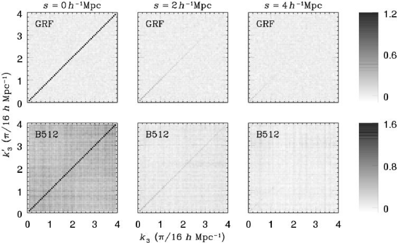
Figure 4.1: Normalized pair-wise covariances $C(k_{3},k_{3}^{\prime};s)$ [see equation (4.2)] in grey scale. The covariances are calculated over 2000 pairs of LOS’s sampled at a fixed separation $s$ from the simulation B512 at $z=3$ (lower panels) and from 2000 GRFs that have the same three-dimensional mass PS as the simulation (upper panels). The grey scale extends to $-0.1$, which corresponds to white.

Figure 4.2: Diagonal elements of the covariance matrix $C(k_{3},k_{3}^{\prime};s)$. The horizontal solid line in the left panel marks the rms value of the off-diagonal elements in the $s=8\ h^{-1}$Mpc case. Other lines are from direct summations of the three-dimensional mass PS using equation (3.3). The symbols are measured from GRFs (left) and the simulation B512 at $z=3$ (right). For GRFs, $C(k_{3},k_{3};0)$ is expected to be unity.

The normalized pair-wise covariance $C(k_{3},k_{3}^{\prime};s)$ is shown in Fig. 4.1 for GRFs and the simulation B512 at $z=3$. The covariances for the GRFs are averaged over an ensemble of 2000 random realizations, while those for the simulation are averaged over 2000 pairs of LOS’s from a single field. The behavior of the covariances is consistent with the expectation. Namely, $C(k_{3},k_{3}^{\prime};0)\simeq\delta^{\rm K}_{n_{3},n_{3}^{\prime}}$ and $C(k_{3},k_{3};s)$ decreases as the separation $s$ increases. The simulation does deviate from GRFs because of the non-Gaussianity, which increases the variance $C(k_{3},k_{3};s)$. Fig. 4.2 compares $C(k_{3},k_{3};s)$ with that from equation (3.3). I note in passing that the expected values of $C(k_{3},k_{3};8\ \mbox{$h^{-1}$Mpc})$ are so close to 0 that they are even below the rms value of the off-diagonal elements of $C(k_{3},k^{\prime}_{3};8\ \mbox{$h^{-1}$Mpc})$ for 2000 GRFs. Hence, it is practically difficult to recover three-dimensional statistics from $\sigma_{\rm 1D}(k_{3},k_{3};s)$ or $\xi(s,k_{3})$ if the LOS’s are too far apart. In theory, the modes of two LOS’s are always correlated as $k\to 0$, regardless of their separation. However, the correlation for $s\gtrsim 8\ h^{-1}$Mpc is so weak that it will not be easily detected against statistical uncertainties. Thus, Figs. 4.1 and 4.2 suggest that LOS’s sampled in a single cosmic density field are practically independent of each other as long as $s\gtrsim 8\ h^{-1}$Mpc.

4.3 Covariance

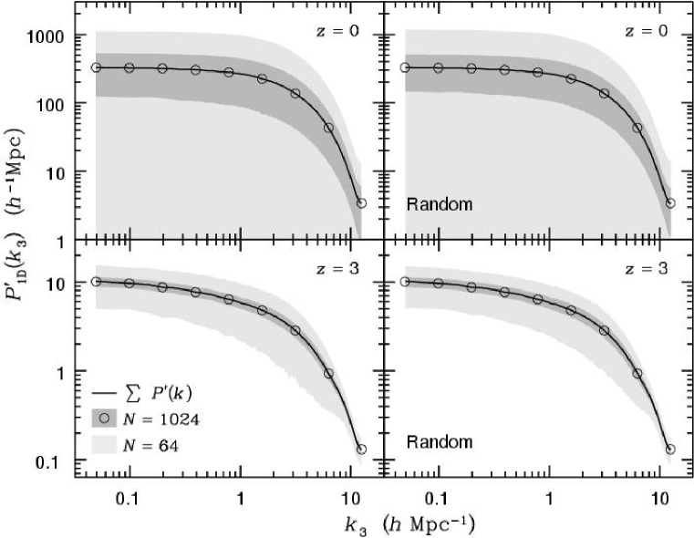
Figure 4.3: Estimated one-dimensional mass PS’s $P^{\prime}_{\rm 1D}(k_{3})$. The PS’s are measured by averaging over 64 (light grey) and 1024 (dark grey) LOS’s that are drawn from the B128 simulation. Shaded areas mark $1\sigma$ dispersion of the PS among 2000 (light grey) and 256 (dark grey, as $256\times 1024$ exhausts all the $512^{2}$ LOS’s) distinct drawings. Circles are the mean PS’s for dark grey areas, i.e. the mean of $512^{2}$ LOS’s. Solid lines are results of a direct summation of the three-dimensional mass PS using equation (4.1). The LOS’s are sampled on a grid with fixed spacing in the left panels but drawn randomly in the right panels.

Fig. 4.3 shows the one-dimensional mass PS measured by averaging over 64 and 1024 LOS’s from the B128 simulation. Although the mean PS of all the $512^{2}$ LOS’s agrees with the result of a direct summation of the three-dimensional mass PS using equation (4.1), the deviation of the PS for any particular group of 64 or 1024 LOS’s is substantial, especially at $z=0$. The variance is smaller at $z=3$ than at $z=0$ because the cosmic density field is more Gaussian earlier on. It is roughly inversely proportional to the number of LOS’s. This can seen better by comparing the lower right panels of Figs. 4.4 and 4.5. However, even at $z=3$ the variance of the one-dimensional mass PS is still much higher than $N^{-1}P_{\rm 1D}^{2}(k_{3})$, i.e. the variance for GRFs, which indicates a heavy contribution from the trispectrum. The formulae in Chapters 2 and 3 often assume that LOS’s are sampled on a grid with fixed spacing, which may not be applicable to realistic data such as inverted densities from the Ly$\alpha$ forest (Nusser & Haehnelt 1999; Zhan 2003). Therefore, I sample the LOS’s in two ways in Fig. 4.3: grid sampling and random sampling. Since no significant difference is observed, random sampling can be safely applied in the rest of this dissertation.

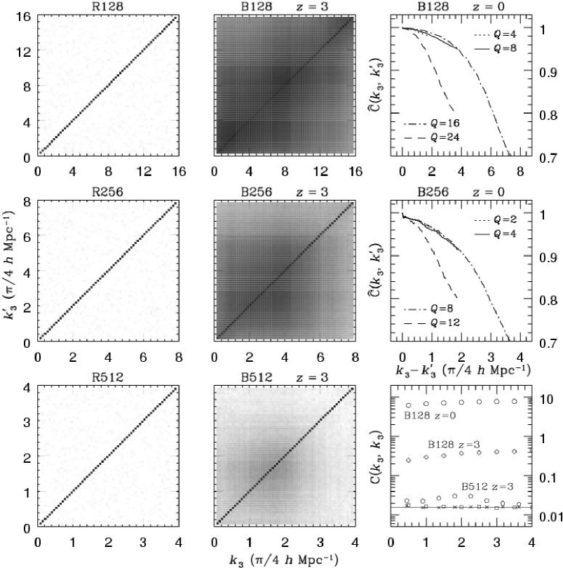
Figure 4.4: Normalized covariances $\hat{C}(k_{3},k^{\prime}_{3})$ [see equation (4.4)] averaged over 2000 groups, each of which consists of 64 LOS’s ($N=64$). For each panel in the left, the LOS’s are randomly drawn from a single GRF that has a box size of 128 $h^{-1}$Mpc (R128), or 256 $h^{-1}$Mpc (R256), or 512 $h^{-1}$Mpc (R512). The GRFs have the same three-dimensional mass PS as their corresponding simulations at $z=0$, but note that $\hat{C}(k_{3},k^{\prime}_{3})$ is independent of redshift for GRFs. Similarly, the middle column is for simulations at $z=3$. The covariances are shown in a linear grey scale with black being $1.2$ and white less than or equal to 0. At $z=0$, the normalized covariances become much less diagonally dominant than the B128 $z=3$ panel in the same grey scale, so only 4 cross sections along $Q=(k_{3}+k_{3}^{\prime})/(\pi/4\ h\ \mbox{Mpc}^{-1})$ are plotted for B128 and B256. Diagonal elements $C(k_{3},k_{3})$ [see equation (4.3)] of R128 (squares), B128 at $z=0$ (circles), B128 at $z=3$ (diamonds), R512 (crosses), and B512 at $z=3$ (pentagons) are shown in the lower right panel along with a thin solid line marking the value $1/64$, i.e. the expectation for GRFs.

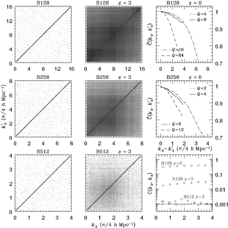
Figure 4.5: The same as Fig. 4.4, except that the normalized covariances $\hat{C}(k_{3},k^{\prime}_{3})$ are averaged over 256 groups, each of which consists of 1024 LOS’s ($N=1024$). The thin solid line in the lower right panel marks the value of $1/1024$.

The normalized covariances $\hat{C}(k_{3},k_{3}^{\prime})$ and $C(k_{3},k_{3}^{\prime})$ are quantified in Figs. 4.4 ($N=64$) and 4.5 ($N=1024$). The left column in each figure is the covariances of the spatially averaged one-dimensional mass PS from a single GRF that has the same box size and three-dimensional mass PS as its corresponding simulation. Clearly, the covariances based on spatial average are nearly diagonal with unity diagonal elements. This is in agreement with the expectations based on ensemble average for GRFs and is consistent with the ergodicity argument. The middle column is similar to the left column except that the density fields are from simulations at $z=3$. The modes in the simulated density fields are strongly correlated, so that the covariances are no longer diagonal. In other words, the trispectrum is non-vanishing for the cosmic density field, as it is the only term that contributes to off-diagonal elements in the covariance. The cosmic density field becomes so non-Gaussian at $z=0$ that grey scale figures of the covariances will not be readable. Hence, I only plot four cross sections perpendicular the diagonal with $Q=(k_{3}+k_{3}^{\prime})/(\pi/4\ h\ \mbox{Mpc}^{-1})$ for B128 and B256 in the right column. The dominance of the diagonals suggested by these cross sections is actually weaker than that in the middle column, which can be seen by contrasting the cross sections for B128 at $z=0$ in Fig. 4.4 with that for B128 at $z=3$ in Fig. 4.6.

The non-Gaussianity is reflected not only in the correlations between different modes but also in the variance of the one-dimensional mass PS, i.e. the diagonal elements of the normalized covariance $C(k_{3},k^{\prime}_{3})$. The lower right panels of Figs. 4.4 and 4.5 compare $C(k_{3},k_{3})$ for five different density fields. The variance from the simulation B128 is orders of magnitude higher than $N^{-1}P^{2}_{\rm 1D}(k_{3})$, and it grows as the non-Gaussianity becomes stronger toward $z=0$. As a result, the sample variance error estimated for GRFs is much lower than what one can actually measure from the cosmic density field. According to equation (3.7), both aliasing and the trispectrum contribute to the variance. Since the GRFs have the same three-dimensional mass PS and are sampled in the same way as the simulations, their near-Gaussian variances of spatially averaged one-dimensional mass PS’s suggest that the contribution of the aliasing effect is negligible. Comparisons of $C(k_{3},k_{3})$ for the same density field but with different sizes of sample ($N=64$ and 1024) confirm the observation in Fig. 4.3 that the variance of the one-dimensional mass PS scales roughly as $N^{-1}$. This means even though the non-Gaussianity drives up the sample variance error of the measured one-dimensional mass PS, one can still reduce the error by sampling a large number of LOS’s.

The distribution function of line-of-sight column densities (upper left panel of Fig. 4.6) suggests that the long tail of high-column-density LOS’s may affect the covariance. I re-calculate the covariance $\hat{C}(k_{3},k_{3}^{\prime})$ with a selection criterion that the column density of each LOS $\rho_{\rm col}/\bar{\rho}_{\rm col}<3$. The result is shown in the upper middle panel of Fig. 4.6. The diagonal elements are more dominant than those in the B128 $z=3$ panel in Fig. 4.4. The first two lower panels are the cross sections of $\hat{C}(k_{3},k_{3}^{\prime})$ with (middle) or without (left) the selection criterion. They provide a more quantitative comparison, which suggests that rare high-column-density LOS’s do increase the correlations between different modes of fluctuations. Meanwhile, Fig. 4.7 clearly demonstrates that these LOS’s also increase the variance of the one-dimensional mass PS by at least a factor of 2 on all scales.

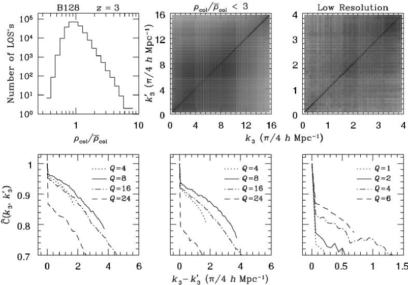
Figure 4.6: The effect of non-Gaussianity and resolution on the covariance. The left column shows the distribution function of column density $\rho_{\rm col}/\bar{\rho}_{\rm col}$ (upper panel) and cross sections of the normalized covariance $\hat{C}(k_{3},k_{3}^{\prime})$ along $Q=(k_{3}+k_{3}^{\prime})/(\pi/4\ h\ \mbox{Mpc}^{-1})$ (lower panel) for B128 at $z=3$. The middle column shows $\hat{C}(k_{3},k_{3}^{\prime})$ (upper panel) and its cross sections (lower panel) for the same simulation output but with an exclusion of 318 LOS’s that have $\rho_{\rm col}/\bar{\rho}_{\rm col}\geq 3$. The normalized covariances in the first two columns are calculated in the same way as in Fig. 4.4, i.e. with 2000 groups and $N=64$. Thus, about half of the 318 LOS’s would be selected without the criterion $\rho_{\rm col}/\bar{\rho}_{\rm col}<3$. The right column is similar to the middle column, but the density is assigned on a grid of $128^{3}$ nodes. All the $128^{2}$ LOS’s are selected and divided into 256 groups with $N=64$. The grey scale is the same as Fig. 4.4.

Figure 4.7: The effect of non-Gaussianity and resolution on the variance, i.e. diagonal elements of the covariance $\sigma^{2}_{\rm 1D}(k_{3},k^{\prime}_{3})$. Diamonds are the normalized variance $C(k_{3},k^{\prime}_{3})$ for B128 at $z=3$. Circles correspond to the middle column of Fig. 4.6, which imposes the selection criterion $\rho_{\rm col}/\bar{\rho}_{\rm col}<3$. Squares are from the low-resolution calculation in the right panel of Fig. 4.6. The horizontal line marks the Gaussian value of $1/64$.

For a fixed number of particles, the simulation box sets a cut-off scale, below which the fluctuations cannot be represented. In other words, the number of particles and the size of the simulation determine the highest-wavenumber modes that are included in calculations of the one-dimensional mass PS and its covariance. Since the non-Gaussianity is stronger at smaller scales, a larger simulation box cuts off more small-scale fluctuations and may cause the correlation to appear weaker in Figs. 4.4 and 4.5. To test this, I assign the density field of the simulation B128 at $z=3$ on a grid of $128^{3}$ nodes. The spatial resolution is the same as the simulation B512 on a grid of $512^{3}$ nodes. The covariance $\hat{C}(k_{3},k_{3}^{\prime})$ is calculated in the same way as those in Fig. 4.4 but with fewer groups of LOS’s. Each group still has 64 LOS’s. The results are shown in the right column of Fig. 4.6 and in Fig. 4.7. Evidently, there is a significant reduction of the correlations between different modes as well as the variance of the one-dimensional mass PS. Indeed, the variance from the low-resolution calculation is close to that from the B512 simulation. Thus, the apparent resemblance between B512 and R512 in Figs. 4.4 and 4.5 is mostly due to the low resolution of the large-box simulation.

It is expected from equation (3.14) that the covariance matrix will not be diagonal if the length of LOS’s is less than the size of the simulation box. Fig. 4.8 shows the covariances that are calculated in the same way as those in Fig. 4.4 for the GRF R512 and the simulation B512, except that each LOS is only 128 $h^{-1}$Mpc long. The effect of the length is not visible for the GRF, but it does increase the correlation between different modes and doubles the variance of the one-dimensional mass PS for the simulation B512. For real observations, the line-of-sight length is always much less than the size of the observable universe, so that the window function in the line-of-sight direction will cause stronger mixing of modes and more pronounced increase of correlation and variance.

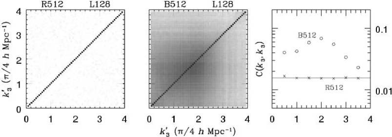
Figure 4.8: The same as the bottom row of Fig. 4.4, but with length of LOS’s $L=128\ h^{-1}$Mpc.

Chapter 5 Covariance of the One-Dimensional Power Spectrum: the Ly$\boldsymbol{\alpha}$ Forest

Previous chapters have focused on the mass PS and its covariance. However, one does not directly observe one-dimensional density fields. What can be observed instead is the Ly$\alpha$ flux. Therefore, many works have been based on flux statistics, which are then used along with simulations to constrain cosmology. Here I examine the flux PS and its covariance using simulated Ly$\alpha$ forests.

5.1 Simulated Ly$\boldsymbol{\alpha}$ Forests

The Ly$\alpha$ forest probes deeply into the nonlinear regime of the cosmic density field. This has made numerical simulations an indispensable tool for understanding the nature of the Ly$\alpha$ forest and inferring cosmological parameters from flux statistics. Two types of cosmological simulations have been commonly used to simulate the Ly$\alpha$ forest. One is pure CDM simulations ($N$-body simulations) that assume baryons to trace dark matter (e.g. Petitjean, Mücket & Kates 1995; Riediger et al. 1998). The other is hydrodynamical simulations (e.g. Cen et al. 1994; Zhang et al. 1995; Hernquist et al. 1996). Other types of simulations exist as well. For example, the simple log-normal model (Bi & Davidsen 1997) is already able to reproduce some Ly$\alpha$ flux statistics.

I use both $N$-body simulations and hydrodynamical simulations to investigate the flux PS and its covariance. Readers are referred to the above references for details of simulation techniques, and I describe the procedure of extracting Ly$\alpha$ forests from simulations in this section.

5.1.1 Hydrodynamical Simulations with Photoionization

Two hydrodynamical simulations (HYDRO1 & HYDRO2) were provided by Romeel Davé. They are both variants of the low-density-and-flat CDM (LCDM) model with a slight tilt of the power spectral index $n$ (see Table 5.1). HYDRO1 evolves $128^{3}$ CDM particles and $128^{3}$ gas particles from $z=49$ to 0 using Parallel TreeSPH (Davé, Dubinski & Hernquist 1997). HYDRO2 differs from HYDRO1 only in cosmological parameters, and it has snapshots available down to $z=2$. The box size is 22.222 $h^{-1}$Mpc in each dimension with a 5 $h^{-1}$kpc resolution. The two simulations also include star formation with feedback and photoionization (Katz, Weinberg & Hernquist 1996). The UV ionization background is from Haardt & Madau (1996).

Table 5.1: Parameters of the simulations.

Model	Type	$\Omega$	$\Omega_{\rm b}^{\ a}$	$\Omega_{\Lambda}$	$h$	$n$	$\sigma_{\mathrm{8}}$
HYDRO1	Hydro.	0.4	0.05	0.6	0.65	0.95	0.8
HYDRO2	Hydro.	0.3	0.04	0.7	0.7	0.95	0.8
HIGH$n$	$N$-Body	0.3	0.04	0.7	0.7	1.1	0.8
HIGH$\sigma$	$N$-Body	0.3	0.04	0.7	0.7	1.0	1.0
LCDM	$N$-Body	0.3	0.04	0.7	0.7	1.0	0.8
OCDM	$N$-Body	0.3	0.04	0	0.7	1.0	0.8

• With exceptions of HYDRO1 & HYDRO2, the baryon density parameter is used only for generating the initial mass power spectrum.

5.1.1.1 Density Grid

Snapshots of the simulations contain the position ${\bf r}_{i}$ and velocity ${\bf v}_{i}$ of each particle, where $i$ is the label of the $i$th particle. Smooth-particle hydrodynamics (SPH) defines the baryon density $\rho_{\rm b}({\bf x})$ at any location to be a sum of contributions from all nearby gas particles, i.e.

$$\rho_{\rm b}({\bf x})=\sum_{i=1}^{N_{\rm p}}m_{i}\,w(|{\bf x}-{\bf r}_{i}|,\epsilon^{j}_{i}),$$ (5.1)

where $N_{\rm p}$ is the total number of particles, $w$ is the density kernel or the assignment function, $m_{i}$ is the mass of particle $i$, and $\epsilon^{j}_{i}$ is the smoothing length determined by the distance between particle $i$ and its $j$th neighbor ($j=32$ in this chapter). In practice, densities are assigned on a discrete grid for further analysis.

I adopt a spherically symmetric spline kernel from Monaghan & Lattanzio (1985, with a typo corrected), which is also used in TreeSPH for force calculations. It has the form

$$w(r,\epsilon)=\frac{1}{\pi\epsilon^{3}}\left\{\begin{array}[]{ll}1-\frac{3}{2}\left(\frac{r}{\epsilon}\right)^{2}+\frac{3}{4}\left(\frac{r}{\epsilon}\right)^{3}&\quad 0\leq r<\epsilon\\ \frac{1}{4}\left[2-\frac{r}{\epsilon}\right]^{3}&\quad\epsilon\leq r<2\epsilon\\ 0&\quad r\geq 2\epsilon,\\ \end{array}\right.$$ (5.2)

which vanishes beyond the radius $2\epsilon$ and has a smooth gradient everywhere. The Fourier transform of the kernel is

$$\hat{w}(k,\epsilon)\equiv\hat{w}(k\epsilon)=\frac{48}{(k\epsilon)^{6}}\left[(4-k\epsilon\sin k\epsilon)\sin^{2}\frac{k\epsilon}{2}-\sin^{2}k\epsilon\right].$$ (5.3)

Fig. 5.1 shows that the density kernel is an effective low-pass filter that suppresses fluctuations on scales smaller than $2\epsilon$ ($k>\pi/\epsilon$). This filtering is necessary because fluctuations on scales less than the physical size of an SPH particle are unphysical. Furthermore, to reduce the alias effect (see Chapter 2), the smoothing length $\epsilon$ is required to be greater than or equal to the spacing of the density grid. Other kernels such as the TSC and wavelet scaling functions have also been used for similar purpose.

Figure 5.1: Fourier transform of the assignment function $w(r,\epsilon)$.

It is important to realize that the filtering scale should be adjusted to particle con-centration—the denser the environment, the smaller the filtering scale. A particle in an empty region does not represent a condensed clump of matter sitting in vacuum but rather a dilute distribution that fills the space between the particle and its distant neighbors. Thus, particles in empty regions should not contribute to small-scale fluctuations. On the other hand, particles in high density regions contain more small-scale information, and their filtering scale should be smaller, i.e. a higher cutoff wavenumber. Density kernels based on neighbor distances satisfy such requirement, and they are widely used in SPH simulations. When the scale of interest is larger than or comparable to the mean inter-particle distance ($k\lesssim k_{\rm p}$, see Chapter 4), kernels with an indiscriminating filtering scale for all particles are just as good. Otherwise, a density-dependent kernel must be used.

The density field $\rho_{\rm b}({\bf x})$ can be readily constructed once the smoothing length is determined for each particle. In principle, LOS’s may be sampled in any random direction, but for computational simplicity I assign the density on a grid of $256^{3}$ nodes, and then extract one-dimensional densities randomly from this grid. Meanwhile, particle temperatures are also assigned to each node with weights proportional to each particle’s contribution of density at that node.

5.1.1.2 Ly$\boldsymbol{\alpha}$ Flux

I assume a universal hydrogen fraction of 0.76 to convert baryon densities to hydrogen densities. For each density node, the equilibrium H i fraction is calculated from the balance between cooling and heating, which include adiabatic cooling (cosmic expansion), photoionization, recombination, collisional excitation and ionization, thermal Bremsstrahlung, and Compton scattering with cosmic microwave background (CMB) photons (for details, see Katz et al. 1996). R. Davé provided codes for this calculation. The assumption of ionization equilibrium certainly breaks down in very dynamic regions such as shocks. However, since the equilibrium H i fraction calculated for shocks is already considerably lower than that elsewhere, there will not be much an effect on simulated Ly$\alpha$ forests even if additional shock physics can further reduce the H i fraction by orders of magnitude. Besides, shock fronts, unlike shocked gases, occupy only a small fraction of the total simulation volume, so they could not have a great impact on the Ly$\alpha$ forest.

With the H i fraction and hydrogen density along the LOS, one can determine the Ly$\alpha$ optical depth $\tau$ and transmitted Ly$\alpha$ flux $F$ of each pixel, i.e. each node of the density grid. The mean flux $\bar{F}$ of all LOS’s is well determined by observations. I adjust the intensity of the UV ionization background $\Gamma_{\rm UV}$ so that the mean flux of all pixels in the simulations follows

$$\bar{F}(z)\simeq\left\{\begin{array}[]{ll}\exp\left[-0.032\,(1+z)^{3.37\pm 0.2}\right]&\quad 1.5\leq z\leq 4\\ 0.97-0.0252\,z\pm(0.003+0.0054\,z)&\quad 0\leq z<1.5,\\ \end{array}\right.$$ (5.4)

which is adapted from Kim et al. (2002) and Davé et al. (1999). This mean flux formula is also consistent with other observations (Lu et al. 1996; Rauch et al. 1997; McDonald et al. 2000). There is a slight inconsistency that HYDRO1 and HYDRO2 have already included the UV ionization background, yet I need to adjust the intensity of the UV radiation on outputs of the simulations to fit mean fluxes. This inconsistency does not significantly affect the results that follow because, first, the simulation outputs are able to reproduce the observed mean flux with their internal UV ionization background (Davé et al. 1999). External adjustments are only needed to vary the mean flux within the given observational and numerical uncertainties. Second, the UV ionization background has an important role in the evolution of the IGM temperature (Katz et al. 1996), but the large-scale distribution of baryons is driven by gravity. Thus, even if the intensities of the externally adjusted UV background were used internally in the simulations, LOS Ly$\alpha$ absorptions should not change greatly.

The mean temperature of the IGM is on the order of $10^{4}$ K, so thermal broadening of absorptions must be taken into account. At a temperature $T_{i}$, the flux decrement $D_{i}=1-F_{i}$ of pixel $i$ is spread to pixel $j$ as

$$D_{ji}=\frac{D_{i}}{\sqrt{\pi T_{4,i}}}\frac{Hd}{b}\int_{j-1/2}^{j+1/2}\,e^{-(i-t)^{2}(Hd)^{2}/b^{2}T_{4,i}}\,{\rm d}t,$$ (5.5)

where $b\simeq 13$ km s^-1, $H$ is the Hubble constant at corresponding redshift, $d$ is the physical separation mapped by two adjacent pixels, and $T_{4,i}=T_{i}/(10^{4}\ \mbox{K})$. The ionization-equilibrium temperature can be uniquely determined from density, and it is obtained for each pixel while H i fraction is calculated recursively. Because of shock heating, especially at low redshift, ionization-equilibrium temperatures are often lower than density-weighted SPH temperatures of the density grid. In this case, the latter is used for thermal broadening. The broadened flux $\widetilde{F}$ is then

$$\widetilde{F}_{i}=1-\sum_{j=1}^{M}D_{ij},$$ (5.6)

where $M$ is the number of pixels along the LOS, but practically the summation is over a much smaller number of pixels where $D_{ij}$ is significant.

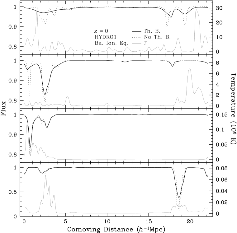
Figure 5.2: Thermal broadening of Ly$\alpha$ absorptions at $z=0$. Solid lines are Ly$\alpha$ absorptions with thermal broadening, and dotted lines without. Grey lines are temperatures along LOS’s. The Ly$\alpha$ forests are generated from baryon distributions in HYDRO1 with the assumption of ionization equilibrium.

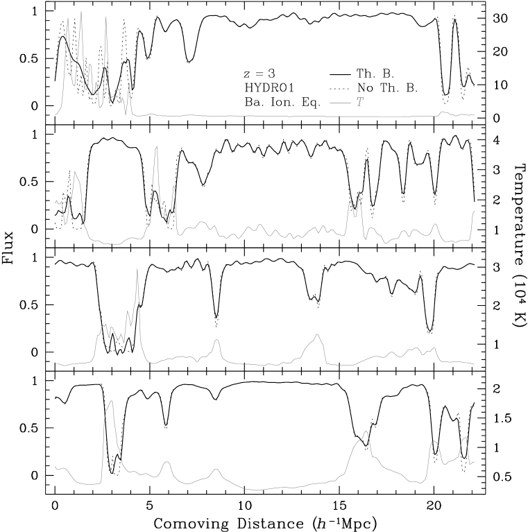
Figure 5.3: Thermal broadening of Ly$\alpha$ absorptions at $z=3$. Legends are the same as in Fig. 5.2.

Thermal broadening smoothes out small-scale fluctuations in the Ly$\alpha$ forest without altering the mean flux. Therefore, it preferentially reduces the flux power on small scales. At $z=3$, the majority of Ly$\alpha$ absorptions arise from regions of density $\rho/\bar{\rho}\lesssim 10$, where temperatures are not much above $10^{4}$ K and broadening widths $b\sqrt{T_{4}}$ are a few tens of km s^-1. At $z=0$, however, Ly$\alpha$ absorptions are produced in much hotter regions where broadening widths can be as high as hundreds of km s^-1. In other words, thermal broadening is a much stronger effect at lower redshift, which can be seen by comparing simulated Ly$\alpha$ forests at $z=0$ (Fig. 5.2) with those at $z=3$ (Fig. 5.3).

There is a general correlation between the temperature and Ly$\alpha$ absorption due to the temperature–baryon density–H i fraction relation (see Section 5.1.2.2). However, high-temperature regions ($T\gtrsim 10^{6}$ K) at $z=0$ are not always related to Ly$\alpha$ absorptions because they are often too hot and too dilute to maintain an appreciable H i column density. These high-temperature regions are categorized as the shock-heated $10^{5}$–$10^{7}$ K WHIM (Davé et al. 1999; Davé & Tripp 2001; Davé et al. 2001).

The cosmic density field becomes more and more clustered so that for any random LOS the chance of passing through relatively high density regions that can produce detectable Ly$\alpha$ absorptions is much smaller at $z=0$. This is reflected in Figs. 5.2 and 5.3 that low-redshift Ly$\alpha$ forests have much fewer absorptions per unit comoving distance than high-redshift ones. It is also interesting to note that there is a relatively deep Ly$\alpha$ absorption in the last panel of Fig. 5.2 despite the high mean flux of 0.97 at $z=0$. The LOS in this panel is the same as that in the second and fourth panels of Fig. 5.5, where LOS baryon and dark matter densities are shown in real space and redshift space, respectively. The deep absorption actually arises from a nearly virialized cluster of real-space density $\rho/\bar{\rho}\sim 160$.

5.1.1.3 Line of Sight in Redshift Space

So far I have not mentioned the fact that the Ly$\alpha$ forest is observed in redshift space where the distribution of matter is distorted by peculiar velocities. A simple way to approximate redshift distortion is to displace each particle a distance $v_{3}/H$ along the LOS before constructing the density grid, i.e.

$${\bf r}^{S}_{i}={\bf r}_{i}+\frac{{\bf v}_{i}\cdot\hat{x}_{3}}{H}\hat{x}_{3},$$ (5.7)

where the superscript $S$ stands for redshift space, and I have made use of the plan-parallel approximation and assumed $\hat{x}_{3}$ to be in the LOS direction. Subsequently, the redshift-space density $\rho^{S}_{\rm b}({\bf x})$ is

$$\rho^{S}_{\rm b}({\bf x})=\sum_{i=1}^{N_{\rm p}}m_{i}\,w(|{\bf x}-{\bf r}^{S}_{i}|,\epsilon^{32}_{i}),$$ (5.8)

where the smoothing length of each particle is also obtained in redshift space. Then, Ly$\alpha$ forests can be extracted from $\rho^{S}_{\rm b}({\bf x})$ in the same way as discussed above. A more detailed discussion on the effect of redshift distortion is given in Section 5.1.2.1.

5.1.2 Pseudo-Hydro Technique

Although full hydrodynamical simulations are well suited for studies of the Ly$\alpha$ forest, they are currently too time-consuming to explore a large cosmological parameter space as one often desires. Whereas, $N$-body simulations run much faster, and they can be used to cover a wide range of cosmological models in practical time.

Croft et al. (1998) proposed a pseudo-hydro technique for generating Ly$\alpha$ forests from $N$-body simulations. It is based on two important theoretical expectations that are supported by hydrodynamical simulations: (1) In general, baryons trace dark matter above the Jeans scale (e.g. Gnedin & Hui 1998); and (2) In ionization equilibrium, the equation of state (EOS) of the IGM gives rise to an approximate temperature–density relation

$$T=T_{0}(\rho_{\rm b}/\bar{\rho}_{\rm b})^{\alpha},$$ (5.9)

where $T_{0}\sim 10^{4}$ K, $0.3\leq\alpha\leq 0.6$, and $\rho_{\rm b}/\bar{\rho}_{\rm b}\lesssim 10$ (Hui & Gnedin 1997). Since the Ly$\alpha$ optical depth is proportional to $\rho_{\rm b}^{2}\,T^{-0.7}$ in regions around the mean density, one finds

$$F\simeq e^{-A(\rho_{\rm b}/\bar{\rho}_{\rm b})^{\gamma}}\simeq e^{-A(\rho_{\rm d}/\bar{\rho}_{\rm d})^{\gamma}},$$ (5.10)

where $A\propto\Omega_{\rm b}^{2}\,\Gamma_{\rm UV}^{-1}T_{0}^{-0.7}$, $\gamma=2-0.7\alpha$, and $\rho_{\rm d}$ is the dark matter density. Usually the constant $A$ is left as a fitting parameter adjusted to reproduce the observed mean flux.

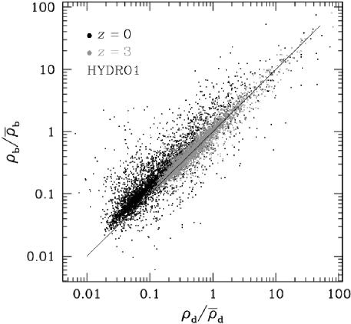
Figure 5.4: The correlation between baryon and dark matter densities. Grey dots are for $z=3$, and black dots $z=0$. Each group consists of 4000 pairs of density values randomly selected from the density grid of the simulation HYDRO1. The diagonal line follows $\rho_{\rm b}/\bar{\rho}_{\rm b}=\rho_{\rm d}/\bar{\rho}_{\rm d}$.

5.1.2.1 Correlation between Baryons and Dark Matter

To justify the pseudo-hydro technique, one must show that baryons and dark matter trace each other on large scales. For a simple test, Fig. 5.4 compares baryon densities with dark matter densities from the same set of 4000 randomly selected density nodes of HYDRO1. There is clearly a strong correlation between baryons and dark matter (see also Gnedin & Hui 1998). The correlation has larger scatter at lower redshift because gravity is no longer the dominant driving force behind strong hydrodynamical events such as shocks, which occur more frequently at lower redshift. Baryons are slightly denser than dark matter below the mean density at $z=0$ because of finite pressure of SPH particles (Gnedin & Hui 1998). In other words, SPH particles have much larger smoothing radii than CDM particles, so that SPH particles in a low-density region receive less acceleration toward a nearby high-density region than CDM particles.

The Jeans length sets a characteristic scale, below which baryon pressure will resist the growth of gravitational perturbations and cause baryons not to trace dark matter. By a simple comparison between the dynamical time and sound travel time, one finds the comoving Jeans length

$$L_{\mathrm{J}} = (1+z)\sqrt{\frac{\pi\,c_{\mathrm{s}}^{2}}{G\rho}}=\sqrt{\frac{40\pi^{2}k_{\mathrm{B}}T}{9\mu m_{\mathrm{p}}H_{\mathrm{0}}^{2}\Omega\,\rho\,(1+z)}}$$ (5.11)

$$= 780\ T_{\mathrm{4}}^{1/2}\left[\Omega\,(\rho/\bar{\rho})(1+z)\right]^{-1/2}\mbox{$h^{-1}$kpc},$$

where $c_{\mathrm{s}}$ is the speed of sound, $G$ is the gravitational constant, $k_{\mathrm{B}}$ is the Boltzmann constant, $\mu\simeq 0.59$ is the mean molecular weight, $m_{\mathrm{p}}$ is the proton mass, and $H_{0}=100\ h$ km s^-1 Mpc^-1. With the EOS equation (5.9), the Jeans length can be rewritten as

$$L_{\mathrm{J}}=780\ \left(\frac{T_{0}}{10^{4}\ {\rm K}}\right)^{1/2}\left[\frac{1}{\Omega\,(1+z)}\right]^{1/2}\left(\frac{\bar{\rho}}{\rho}\right)^{(1-\alpha)/2}\mbox{$h^{-1}$kpc}.$$ (5.12)

For $T_{0}=10^{4}$ K and $\Omega=0.4$ (HYDRO1), it is expected that baryons in regions around the mean density to generally follow dark matter above 1.2 $h^{-1}$Mpc (0.6 $h^{-1}$Mpc) at $z=0$ ($z=3$). Of course, in vast low density regions the Jeans length may be much larger.

The Jeans length analysis idealizes the state of baryons and neglects external forces. Thus, it is not applicable in very dynamic regions such as shock fronts. For example, in the spherical collapse case, even though baryons may initially follow dark matter, shocks could eventually develop and allow baryons to separate from dark matter.

Figure 5.5: LOS baryon densities (dashed liens) and dark matter densities (solid lines) at $z=0$. The upper two panels show LOS’s in real space, while the lower two the same LOS’s in redshift space. All densities are extracted from HYDRO1. The two LOS’s here correspond to those in the second and last panels of Fig. 5.2.

Figure 5.6: The same as Fig. 5.5 but at $z=3$. The two LOS’s here correspond to those in the second and last panels of Fig. 5.3.

Figs. 5.5 and 5.6 examine baryon and dark matter densities along LOS’s in both real space and redshift space. The two LOS’s in Fig. 5.5 (Fig. 5.6) correspond to the LOS’s in the second and last panels of Fig. 5.2 (Fig. 5.3). Baryon densities and dark matter densities have almost one-to-one correspondence in real space at $z=3$. However, they do not share the same velocity structure because SPH particles receive not only gravitational accelerations but also hydrodynamical accelerations. This leads to the departure of baryons from dark matter in redshift space. At $z=0$, the difference between baryon and dark matter distributions is already seen in real space, and it does not seem to be amplified by redshift distortion.

Figure 5.7: Three-dimensional and one-dimensional mass PS’s of baryons (dashed lines) and dark matter (solid lines) from HYDRO1. Redshift-space PS’s are shown in thick lines, and real-space PS’s thin lines.

The LOS densities of baryons and dark matter are qualitatively consistent with the expectation from Jeans length analysis, and statistics are needed to quantify how well baryons and dark matter trace each other. Fig. 5.7 compares baryon and dark matter PS’s in both real space and redshift space. At $z=3$, the three-dimensional baryon PS has already departed from the three-dimensional dark matter PS on scales below 6 $h^{-1}$Mpc ($k\gtrsim 1$ $h$ Mpc^-1), which is ten times larger than the Jeans length in mean-density regions. This discrepancy can be attributed to the fact that the vast volume of the universe is well below the mean density and have much larger Jeans lengths. Therefore, the three-dimensional baryon PS is somewhat lower than that of dark matter for $k\gtrsim 1$ $h$ Mpc^-1, even though the Jeans length in mean-density regions corresponds to $k_{\rm J}\simeq 10$ $h$ Mpc^-1. At $z=0$, shocks have heated parts of the IGM to much higher temperatures and led to more reduction of the baryon PS with respect to the dark matter PS.

The linear redshift distortion is first derived by Kaiser (1987),

$$P^{S}({\bf k})=\left(1+\beta\,\mu^{2}_{\theta}\right)^{2}P({\bf k}),$$ (5.13)

where $P^{S}({\bf k})$ is the three-dimensional mass PS in redshift space, $\beta\simeq\Omega^{0.6}(z)$ (Lahav et al. 1991), and $\mu_{\theta}$ is the cosine of the angle between the LOS and the wavevector ${\bf k}$. The monopole of $P^{S}({\bf k})$ is

$$P^{S}_{0}(k)=\Big{(}1+\frac{2}{3}\beta+\frac{1}{5}\beta^{2}\Big{)}P(k),$$ (5.14)

which is boosted with respect to $P(k)$ by a factor of 1.9 at high redshift. The nonlinear redshift distortion reduces the power of Fourier modes along the LOS, and the reduction is more severe on smaller scales. These effects are illustrated in Fig. 5.7. Both the constant boost on large scales and the reduction of power on small scales can be seen from three-dimensional mass PS’s at $z=3$. Whereas, the nonlinear scale of redshift distortion has evolved beyond the size of the simulation box at $z=0$, so that the monopole of the redshift-space PS is always below the real-space PS. The nonlinear redshift distortion is also reflected in Fig. 5.5, where a real-space structure of $\rho/\bar{\rho}\sim 160$ is smoothed to $\rho/\bar{\rho}\sim 20$ in redshift space. Since the nonlinear redshift distortion is equivalent to a small-scale filter, differences between PS’s are expected to be smaller in redshift space than in real space. However, the agreement of $P^{S}_{0}(k)$ between baryons and dark matter at $z=3$ is probably coincidental.

The real-space one-dimensional PS of baryons can differ significantly from that of dark matter even on large scales, because the one-dimensional mass PS is an integral of the three-dimensional mass PS. The difference should be a constant on scales that baryons have exactly the same three-dimensional PS as dark matter. In redshift space, the one-dimensional mass PS is

$$P^{S}_{\rm 1D}(k_{3})=\frac{1}{4\pi^{2}}\int_{0}^{\infty}P^{S}({\bf k}_{\perp},k_{3})\,{\rm d}{\bf k}_{\perp}.$$ (5.15)

The anisotropy of the redshift-space three-dimensional mass PS has made redshift distortion less intuitive for the one-dimensional mass PS.

5.1.2.2 Equation of State

Fig. 5.8 demonstrates the correlation between temperature and baryon density for the simulation HYDRO1. The temperature–density relation is fairly tight at $z=3$, and it follows the EOS $T=T_{0}(\rho_{\rm b}/\bar{\rho}_{\rm b})^{0.6}$ closely. Two theoretical temperature–density curves for ionization equilibrium at $z=3$ are also provided in Fig. 5.8. The UV background intensities of the two curves are adjusted to fit mean fluxes of $0.77$ and $0.64$. Although the UV intensities differ by a factor of 2.5, there is no visible difference between the two curves at $\rho_{\rm b}/\bar{\rho}_{\rm b}<5$. Compared to the simulation and the curves of ionization equilibrium, the simple EOS is indeed a good approximation.

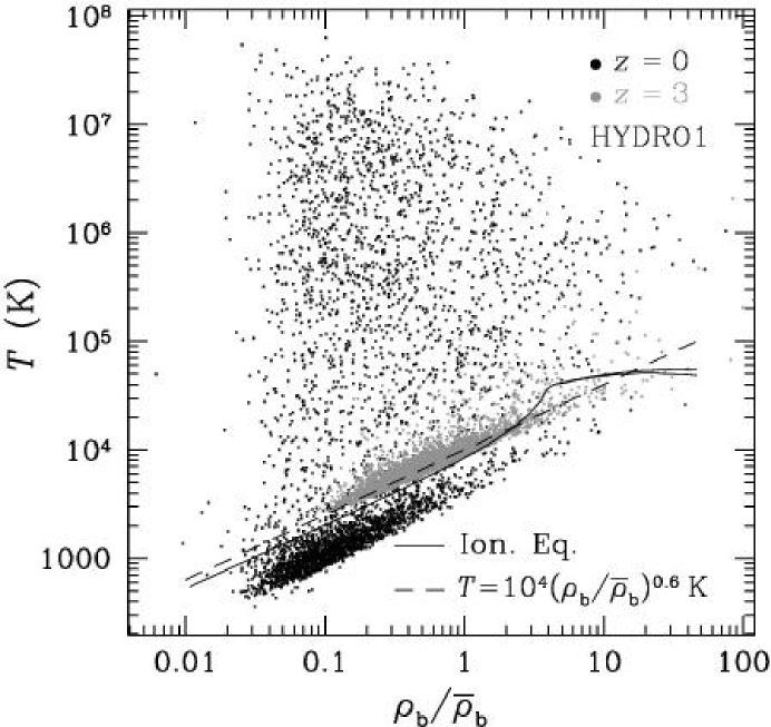
Figure 5.8: The temperature–density relation of baryons. Grey dots are for $z=3$, and black dots $z=0$. Each group consists of 4000 pairs of temperature and density values randomly selected from the density grid of HYDRO1. The dashed line represents an EOS $T=10^{4}(\rho_{\rm b}/\bar{\rho}_{\rm b})^{0.6}$ K. The solid lines are calculated from ionization equilibrium with a factor of 2.5 difference in the UV background intensity.

At $z=0$, the IGM develops multiple phases; the bulk of the IGM has become cooler, while some gases are shock-heated to temperatures up to a few times $10^{7}$ K—the WHIM. These WHIM gases are generally too hot and too dilute to produce appreciable Ly$\alpha$ absorptions. They explain why many high-temperature regions at $z=0$ (see the first two panels of Fig. 5.2) do not correspond to any absorptions at all, even though high-temperature regions would be naively thought of as high-density regions from the simple EOS.

Note that the temperatures and densities in Fig. 5.8 are randomly selected from the density grid. Since smoothing lengths of SPH particles are required to be at least the size of the grid spacing, one will not get a high-density tail that is often seen in a particle temperature–particle density plot. The sharp edges of temperature–density distributions are due to the internal UV background of the simulation, which keeps SPH particles from cooling below the ionization-equilibrium temperature.

5.1.2.3 Variants of the Pseudo-Hydro Technique

Table 5.2: Methods for generating the Ly$\alpha$ forest.

Method	Particle	$\rho_{\rm b}$	$T_{\rm th}^{\ \ a}$	$\tau$
BI	SPH		Max$[T_{\rm sph},T_{\rm ie}(\rho_{\rm b})]$	Ion. Eq.
BE	SPH		$T_{0}(\rho_{\rm b}/\bar{\rho}_{\rm b})^{\alpha}$	$\propto(\rho_{\rm b}/\bar{\rho}_{\rm b})^{\gamma}$
DI	CDM	$\propto\rho_{\rm d}$	$T_{\rm ie}(\rho_{\rm b})$	Ion. Eq.
DE	CDM	$\propto\rho_{\rm d}$	$T_{0}(\rho_{\rm b}/\bar{\rho}_{\rm b})^{\alpha}$	$\propto(\rho_{\rm b}/\bar{\rho}_{\rm b})^{\gamma}$

• $T_{\rm th}$ is the temperature used for thermal broadening, $T_{\rm sph}$ is the grid temperature based on temperatures of SPH particles in hydrodynamical simulations, and $T_{\rm ie}(\rho_{\rm b})$ is the ionization-equilibrium temperature of a gas with density $\rho_{\rm b}$.

Separately, Petitjean et al. (1995) developed a slightly different pseudo-hydro technique. They assume baryons to trace dark matter but do not use the simple EOS. Temperatures and optical depths of baryons are calculated from ionization equilibrium in their method (labeled as DI). As seen in Fig. 5.8, the ionization-equilibrium temperature is usually lower than the density-weighted SPH temperature. As such, small-scale fluctuations may not be sufficiently filtered by thermal broadening in this method.

One may devise another variant of the pseudo-hydro technique by applying the simple EOS and equation (5.10) to baryons in hydrodynamical simulations. I refer to this method as BE and that of Croft et al. (1998) DE. Similarly, the name BI is given to the full-hydrodynamical approach described in Section 5.1.1. One can assess the importance of shocks by comparing methods BE with BI, while the difference between methods BE and DE must arise from the difference between baryon distributions and dark matter distributions. The four methods are summarized in Table 5.2.

Figure 5.9: Transmitted Ly$\alpha$ flux based on baryon and dark matter distributions at $z=0$. The three panels compare the same Ly$\alpha$ forest generated from baryons in ionization equilibrium (BI) to those from baryons with an EOS (BE), dark-matter-converted baryons in ionization equilibrium (DI), and dark-matter-converted baryons with an EOS (DE). All the four methods are required to reproduce the same mean flux of $0.97$.

Figure 5.10: The same as Fig. 5.9, except that Ly$\alpha$ forests are generated from baryon and dark matter distributions at $z=3$ and the mean flux is $0.71$.

5.1.3 Comparison

To give a visual impression of pseudo-hydro techniques, I show in Figs. 5.9 and 5.10 Ly$\alpha$ forests obtained along the same LOS using the four methods, BI, BE, DI, and DE. The mean flux over all $256^{2}$ Ly$\alpha$ forests by the four methods are required to match the observed mean flux of $0.97$ at $z=0$ and $0.71$ at $z=3$, but the mean flux of a single LOS is not necessarily the same across the methods. Since a simple EOS does not take into account the substantial amount of WHIM at $z=0$ (see Fig. 5.8), pseudo-hydro techniques are expected to be less accurate at lower redshift. This is seen in Fig. 5.9. On the other hand, at $z=3$, methods involving ionization equilibrium and the EOS generate almost identical Ly$\alpha$ forests, and the difference between Ly$\alpha$ forests generated from baryons and those from dark matter is also small.

Fig. 5.11 evaluates the statistical performance of pseudo-hydro techniques using flux PS’s. Grey bands are $1\sigma$ dispersions of flux PS’s of Ly$\alpha$ forests produced using the method BI. The dispersions are calculated among 1000 groups, each of which contains 64 LOS’s randomly selected with no repetition. There is a good agreement among all methods at $z=3$, but all the three pseudo-hydro methods, BE, DE, and DI fail to converge on BI at $z=0$. The method DI seems to work better than the other two on scales $k<5$ $h$ Mpc^-1 at $z=0$. The excess of flux power for pseudo-hydro techniques is expected because they all underestimate the IGM temperature and produce more flux fluctuations than the full-hydro method (see Figs. 5.8 and 5.9). In fact, methods BI and BE have identical baryon distributions, so that the difference in their flux PS’s can only be attributed to the IGM temperature. Hence, one concludes that the temperature structure of the IGM is critical to the Ly$\alpha$ forest and flux PS at low redshift.

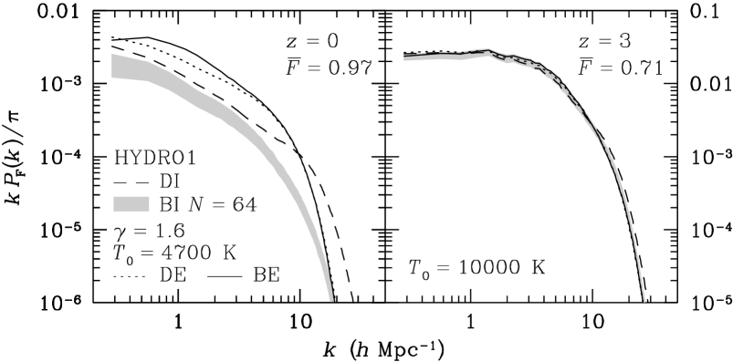
Figure 5.11: Flux PS’s of Ly$\alpha$ forests at $z=0$ and $z=3$. The Ly$\alpha$ forests are produced using the four methods listed in Table 5.2. Grey bands represent $1\sigma$ dispersions of flux PS’s of Ly$\alpha$ forests generated from baryons in ionization equilibrium. The dispersions are calculated among 1000 groups, each of which consists of 64 LOS’s.

The mean-density temperature of the IGM $T_{0}$ does not affect the optical depth in methods BE and DE because it is absorbed into the parameter $A$ in the approximation $F=\exp\left[-A(\rho/\bar{\rho})^{\gamma}\right]$, which is adjusted to fit the observed mean flux. However, $T_{0}$ can affect simulated Ly$\alpha$ forests through thermal broadening as indicated by the fast drop of the flux PS’s for methods BE and DE. To test this, I reproduce Ly$\alpha$ forests using $T_{0}=15000$ K, which is roughly three times (1.5 times) the mean-density temperature of the IGM in HYDRO1 at $z=0$ ($z=3$). Flux PS’s of these Ly$\alpha$ forests are shown in Fig. 5.12. One sees that the higher mean-density temperature reduces more flux power on small scales while leaving flux PS’s unchanged on large scales. As such, the flux PS is less robust on small scales as a constraint for cosmology. The small-scale excess of flux power for the method DI with respect to BI is also due to thermal broadening because the ionization-equilibrium temperature is almost always lower than the density-weighted temperature of SPH particles.

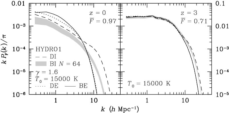
Figure 5.12: The same as Fig. 5.11, except that for methods BE and DE Ly$\alpha$ forests are generated with $T_{0}=15000$ K. Methods BI and DI are not affected by $T_{0}$.

5.2 Tuning the Ly$\boldsymbol{\alpha}$ Forest

It is already seen in last section that pseudo-hydro techniques do not work well at low redshift and their performances are not all equal. Simulated Ly$\alpha$ forests are affected by many elements including, for instance, the EOS (for methods BE and DE) and the mean flux. If they are to be compared with the statistics of observed Ly$\alpha$ forests and to be used to determine cosmological parameters, one must understand the dependence of the statistics of simulated Ly$\alpha$ forests on the above-mentioned elements.

5.2.1 Equation of State

The EOS maps density fluctuations to flux fluctuations by relating optical depths to densities. For a given density and mean flux, different EOS’s will assign different optical depths, which alters amplitudes of flux fluctuations and, therefore, the flux PS.

For a stiff EOS, i.e. a small value of $\gamma$, high-density regions have to absorb less Ly$\alpha$ flux, while, in compensation, low-density regions have to absorb more. In terms of flux, a stiff EOS leads to higher fluxes in deep (or large-equivalent-width) absorptions and lower fluxes in shallow absorptions than a soft EOS does. This expectation is confirmed in Figs. 5.13 and 5.14, where Ly$\alpha$ forests generated using methods BE and DE are compared with those using the method BI at $z=0$, 1, 2, and 3. The mean flux is kept the same for all the methods used here at each epoch, while only the EOS is varied. The value of $\gamma=1.4$ in the figures corresponds to an unrealistically stiff EOS, and it is provided only for the purpose of comparison.

Figs. 5.13 and 5.14 show that low-amplitude and small-scale fluctuations in the flux are likely to be suppressed for methods BE and DE, while high-amplitude fluctuations are likely to be amplified. Overall, this boosts the flux PS on large scales with respect to that of the method BI as observed in Fig. 5.11. Although methods BE and DE are not good approximations at low redshift, they work remarkably well with $\gamma=1.6$ at $z=3$.

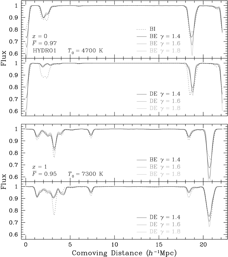
Figure 5.13: Ly$\alpha$ Forests generated from baryon and dark matter distributions with different EOS’s. The upper two panels are for $z=0$, and the lower two $z=1$. The Ly$\alpha$ forests are produced from baryon densities and dark matter densities using $F=\exp[-A(\rho/\bar{\rho})^{\gamma}]$, where $A$ is adjusted to fit the mean flux $\bar{F}$. Thermal broadening is included with temperature given by $T=T_{0}(\rho/\bar{\rho})^{\alpha}$.

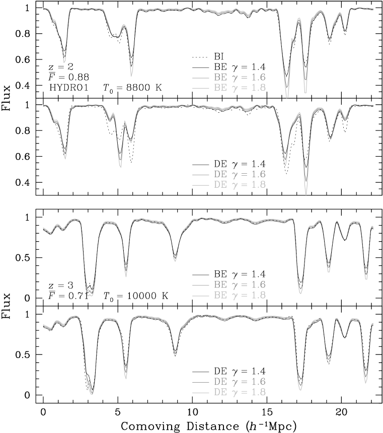
Figure 5.14: The same as Fig. 5.13, except that the upper two panels are for $z=2$, and the lower two $z=3$.

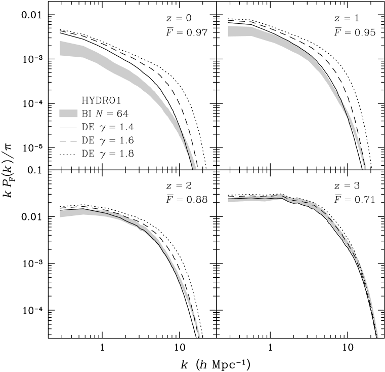
Figure 5.15: Flux PS’s of Ly$\alpha$ forests generated from dark-matter-converted baryon densities using different EOS’s. Grey bands represent $1\sigma$ dispersions of the flux PS’s of Ly$\alpha$ forests generated from baryons in ionization equilibrium. The dispersions are calculated in the same way as in Fig. 5.11.

Since the amplitude of flux fluctuations increases with $\gamma$ in Figs. 5.13 and 5.14, a smaller value of $\gamma$ must lead to a lower flux PS. This is observed in Fig. 5.15, where flux PS’s of Ly$\alpha$ forests obtained using the method DE with different EOS’s are compared with those using the method BI. Methods DE and BE produce very similar Flux PS’s, so flux PS’s of method BE are not shown separately. Fig. 5.15 demonstrates that one cannot tune the EOS to make pseudo-hydro techniques work at low redshift. Meanwhile, pseudo-hydro techniques appear to be a good approximation for studies of the flux PS at $z=3$. The difference among different EOS’s is also less pronounced at $z=3$, because the dynamical range of $\rho/\bar{\rho}$ is much smaller.

5.2.2 Mean Flux

The mean flux affects the Ly$\alpha$ forest and the flux PS in a simple way. Low-density regions of the IGM cannot absorb much Ly$\alpha$ flux no matter what mean flux is required. Thus, the mean flux mostly affects regions where absorption is already significant. Specifically, a higher mean flux weakens existing absorptions and decreases the flux PS over all scales. The Ly$\alpha$ forest should be more sensitive to the mean flux at lower redshift when Ly$\alpha$ absorptions often arise from denser regions.

Fig. 5.16 compares Ly$\alpha$ forests obtained along the same LOS but with different mean fluxes given by observational and simulational uncertainties [see equation (5.4)]. Since all the four methods in Table 5.2 have the same dependence on the mean flux, I only show flux PS’s of Ly$\alpha$ forests generated using the full-hydro method. As expected, the mean flux monotonically alters Ly$\alpha$ forests in all regions with greater changes in deeper absorptions, and a lower mean flux gives rise to stronger fluctuations in the flux. If one takes into account that the difference in the mean fluxes at $z=0$ is about 20 times smaller than that at $z=3$, the low-redshift Ly$\alpha$ forest does seem to be more sensitive to the mean flux.

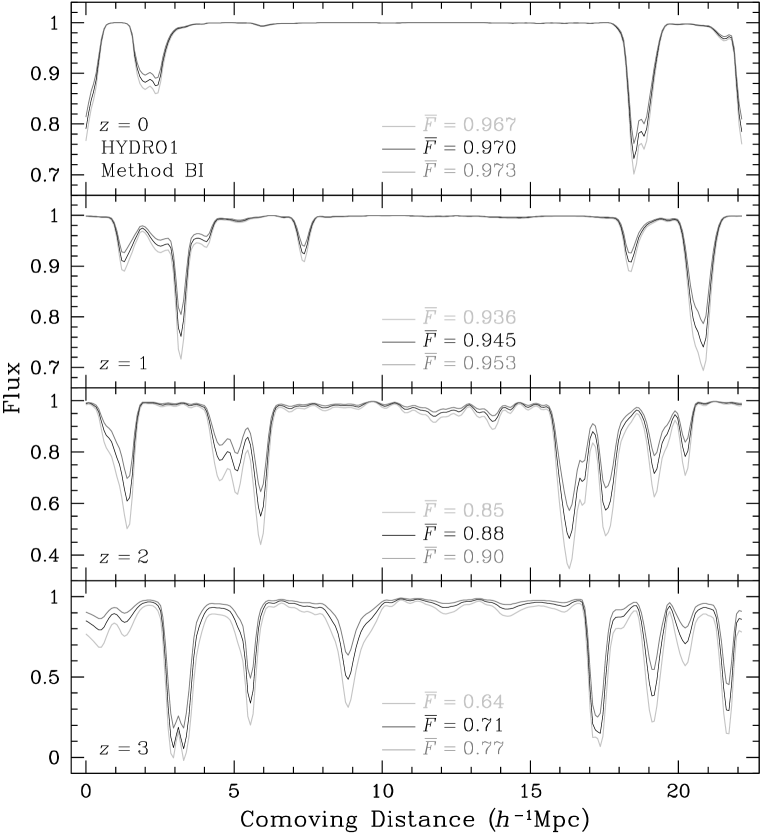
Figure 5.16: Simulated Ly$\alpha$ forests with mean fluxes from equation (5.4). The Ly$\alpha$ forests are generated from baryons in ionization equilibrium. Note that the difference in mean fluxes increases with redshift.

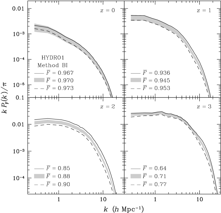
Figure 5.17: Flux PS’s of simulated Ly$\alpha$ forests with mean fluxes from equation (5.4). The Ly$\alpha$ forests are generated from baryons in ionization equilibrium. The grey band in each panel is the $1\sigma$ dispersion of the flux PS with the medium mean flux. The dispersions are calculated among 1000 groups, each of which consists of 64 LOS’s.

Fig. 5.17 shows that flux PS’s are also monotonically altered by the mean flux. A lower mean flux (more absorptions) leads to a higher flux PS on all scales. Unlike the EOS, the mean flux does not change the shape of the flux PS much. This implies that the mean flux can uniquely determine the normalization of the flux PS. In other words, the mean flux is a relatively robust constraint on simulated Ly$\alpha$ forests.

5.3 Mass Statistics vs. Flux Statistics

5.3.1 Power Spectrum

The Ly$\alpha$ forest has been used to infer the linear mass PS of the cosmic density field. The nonlinear transform of the density to the flux has made it difficult to derive the mass PS from the flux PS analytically. One way to circumvent the difficulty is to use simulations to map the flux PS to the mass PS (Croft et al. 2002). As such, it is important to compare the flux PS with the mass PS.

Plotted in Figs. 5.18 and 5.19 are flux PS’s of Ly$\alpha$ forests produced from baryons and dark-matter-converted baryons in ionization equilibrium along with one-dimensional mass PS’s of baryons and dark matter. One $\sigma$ dispersions of baryon flux PS’s and mass PS’s are shown in grey. The most prominent feature is that one-dimensional mass PS’s have much larger dispersions than flux PS’s. As discussed in Chapter 4, the variance in the one-dimensional mass PS is severely inflated by the trispectrum of the cosmic density field because of the non-Gaussianity.

An interesting observation is that unlike the mass PS the flux PS decreases with time. This is due to the thinning of the Ly$\alpha$ forest and the higher mean flux toward lower redshift that reduce fluctuations in the Ly$\alpha$ flux.

The nonlinear transform between baryon density and flux greatly suppresses the fluctuations. For example, the overdensity $\delta$ may vary from -1 to hundreds (tens) at $z=0$ ($z=3$), but the flux can only be between 0 and 1. With a mean flux on the order of unity, fluctuations in the flux are $10$–$10^{2}$ times weaker than those in the cosmic density field. Hence, the flux PS is a factor of $10^{2}$ ($z=3$) to $10^{4}$ ($z=0$) times lower than the one-dimensional mass PS. Moreover, the non-Gaussianity in the cosmic density field is even more suppressed in the flux because it is a higher-order effect. Thus, the flux trispectrum is much closer to zero as compared to the mass trispectrum of the cosmic density field, and the variance of the flux PS becomes much smaller than the variance of the one-dimensional mass PS.

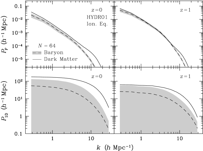
Figure 5.18: Flux PS’s of simulated Ly$\alpha$ forests and one-dimensional mass PS’s of the underlying density fields at $z=0$ and $1$.

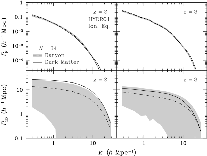
Figure 5.19: Flux PS’s of simulated Ly$\alpha$ forests and one-dimensional mass PS’s of the underlying density fields at $z=2$ and $3$.

The near-Gaussian Ly$\alpha$ flux is probably the reason that many simulations and techniques are able to reproduce lower-order statistics of the observed Ly$\alpha$ forest, especially at high redshift. A potential problem arises because of Figs. 5.18 and 5.19. That is one could produce Ly$\alpha$ forests from wildly different density fields but still have almost identical flux PS. For instance, even though baryons and dark matter differ considerably in terms of mass PS (see also Fig. 5.7), they are not so distinguishable from each other in flux PS’s at $z\geq 2$. Conversely, we are able to measure the flux PS extremely well, but how much confidence do we have in recovering the underlying mass PS?

5.3.2 Covariance

Higher-order statistics may be able to break the degeneracy. Here I employ the covariance of the one-dimensional PS to explore the difference between Ly$\alpha$ forests generated using the full-hydro method BI and those using the pseudo-hydro method DI.

Figs. 5.20 and 5.21 illustrate normalized covariances $\hat{C}(k_{3},k^{\prime}_{3})$ and $C(k_{3},k^{\prime}_{3})$ of one-dimensional mass PS’s and flux PS’s, respectively, at $z=0$. The covariances are calculated from 1000 groups, each of which consists of 64 LOS’s ($N=64$) randomly selected from the density grid of HYDRO1. For GRFs, both $\hat{C}(k_{3},k^{\prime}_{3})$ and $C(k_{3},k^{\prime}_{3})$ are diagonal with $\hat{C}(k_{3},k^{\prime}_{3})=\delta^{\rm K}_{n_{3},n^{\prime}_{3}}$ and $C(k_{3},k^{\prime}_{3})=N^{-1}\delta^{\rm K}_{n_{3},n^{\prime}_{3}}$. For better comparison, the covariances $C(k_{3},k^{\prime}_{3})$ are multiplied by $N$, so that the Gaussian case has $N\,C(k_{3},k^{\prime}_{3})=\delta^{\rm K}_{n_{3},n^{\prime}_{3}}$. As already seen in Chapter 4, the covariances of one-dimensional mass PS’s are starkly non-Gaussian. The normalized variances $C(k_{3},k_{3})$ are two orders of magnitude higher than expected for GRFs. The covariances of baryons are roughly a factor of 2 lower than those of dark matter. This is likely due to the larger smoothing radii of SPH particles that filter out more small-scale non-Gaussian fluctuations. The covariances of flux PS’s have a dominant diagonal, though they are still not Gaussian. The difference in the covariances between the full-hydro method BI and the pseudo-hydro method DI is comparable to the difference in their flux PS’s. The method BI gives rise to stronger correlations between high-$k$ modes in the flux PS than the method DI does because of the WHIM.

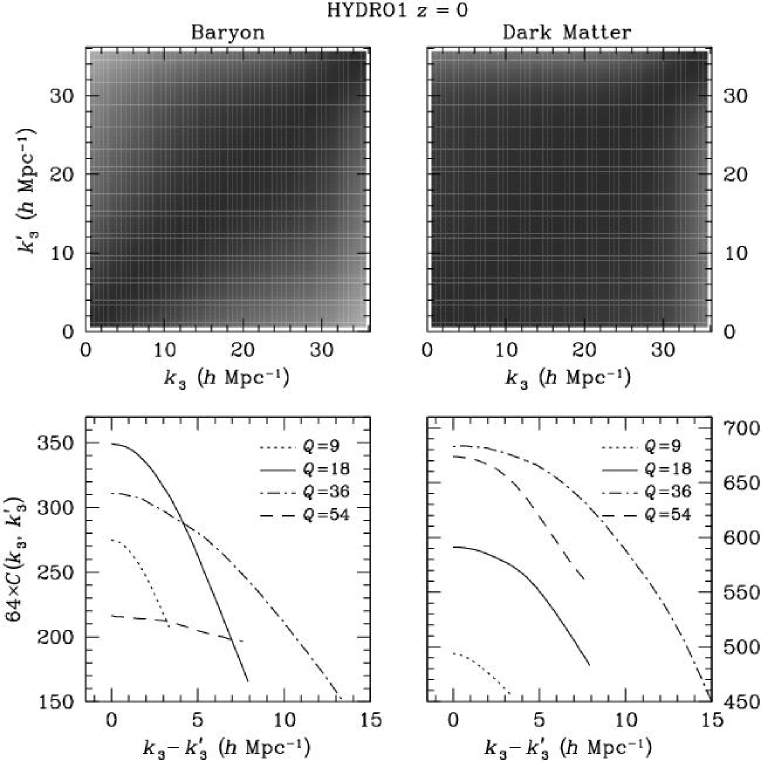
Figure 5.20: Normalized covariances of one-dimensional baryon and dark matter PS’s at $z=0$. The upper panels are covariances $\hat{C}(k_{3},k^{\prime}_{3})$ in the same grey scale as Fig. 4.4. The lower panels are cross sections of covariances $C(k_{3},k^{\prime}_{3})$ along $Q=(k_{3}+k^{\prime}_{3})/\mbox{$h^{-1}$Mpc}$. The covariances $C(k_{3},k^{\prime}_{3})$ are multiplied by 64 for better comparison with that of GRFs, which follows $64\,C(k_{3},k^{\prime}_{3})=\delta^{\rm K}_{n_{3},n^{\prime}_{3}}$. All the covariances are calculated from 1000 groups, each of which consists of 64 LOS’s ($N=64$) randomly selected from the density grid of HYDRO1.

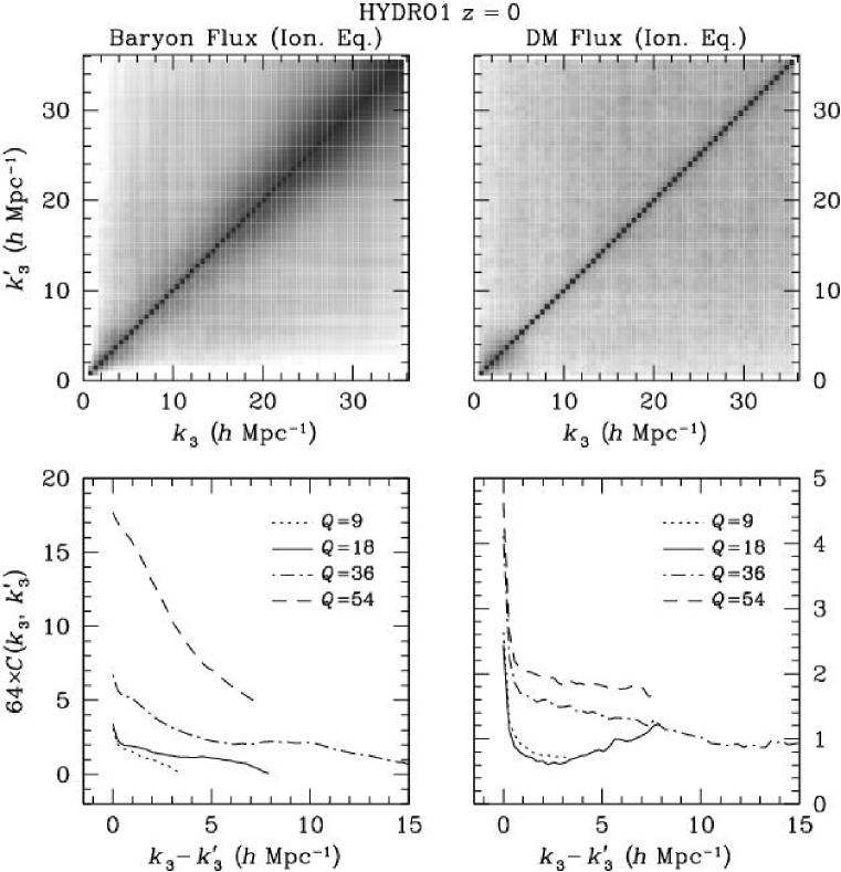
Figure 5.21: The same as Fig. 5.20, but for flux PS’s of Ly$\alpha$ forests generated from baryons and dark matter using methods BI and DI.

Figs. 5.22 and 5.23 present normalized covariances of one-dimensional mass PS’s and flux PS’s for the simulation HYDRO2 at $z=3$, which are very similar to those for HYDRO1. At this redshift, the covariances of one-dimensional mass PS’s are reduced by a factor of a few, but they are still highly non-Gaussian. Whereas, the covariances of flux PS’s are very close to Gaussian, and the difference between the two methods BI and DI is greatly reduced compared to that at $z=0$.

In addition to simulations, I show in Fig. 5.24 normalized covariances of observed flux PS’s at $z=3$. The sample of Ly$\alpha$ forests includes 20 QSO spectra from Bechtold (1994) and Dobrzycki & Bechtold (1996). The QSO spectra are selected so that each contains at least one good chunk of spectrum that has no bad pixels or strong metal lines and spans 64 Å anywhere within $z=2.9$–$3.1$. The spectral resolution is 1 Å, which is about four times lower than that in the simulations. In all, there are 27 segments of Ly$\alpha$ forests for the analysis. I do not re-group the segments, i.e. $N=1$, in calculating the covariances.

The main characteristics of the observed covariances are in good agreement with simulated ones. Namely, the normalized covariance matrices have a strongly dominant diagonal, and they are very close to Gaussian. The values of diagonal elements seem to match those in simulations, but the off-diagonal elements are a little noisier because of the small sample size. With a large number of high-resolution Ly$\alpha$ forests, one will be able to study the behavior of the covariance on smaller scales (larger $k$) and reduce statistical uncertainties.

A general observation of covariances of flux PS’s is that the correlation between two LOS modes decreases away from the diagonal, since two neighboring modes are more likely to be correlated than two distant modes. Beyond this point, however, the behavior of the covariances is not quantitatively understood. It also seems that the covariance of the flux PS does not provide more leverage for differentiating the underlying density field than the flux PS itself. This echos the finding by Mandelbaum et al. (2003) that the flux trispectrum does not provide much extra information than the flux PS.

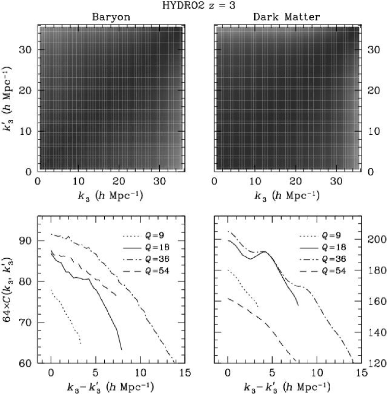
Figure 5.22: The same as Fig. 5.20, but for the simulation HYDRO2 at $z=3$.

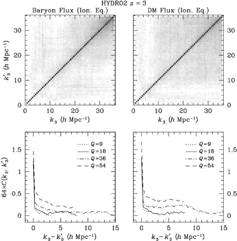
Figure 5.23: The same as Fig. 5.22, but for flux PS’s.

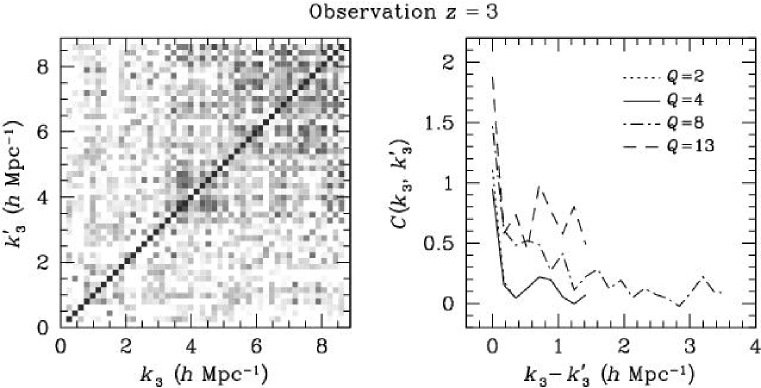
Figure 5.24: The same as Fig. 5.23, but for observed Ly$\alpha$ forests. The covariances are calculated from 27 segments of Ly$\alpha$ forests with $N=1$. Note that the resolution of the observed Ly$\alpha$ forests is about four times lower than that in the simulations.

5.4 Cosmology

Because of the difficulty in deriving density statistics from flux statistics, one often resorts to numerical simulations and constrains cosmology by comparing observed flux statistics directly to simulated flux statistics. In addition, one utilizes fast $N$-body simulations and pseudo-hydro techniques in order to explore a large cosmological parameter space in manageable time. This necessitates an examination of the accuracy of pseudo-hydro techniques and the sensitivity of flux statistics to cosmology.

Figs. 5.25 and 5.26 compare mass PS’s and flux PS’s for six simulations: HYDRO1, HYDRO2, LCDM, high-$n$ LCDM (HIGH$n$), high-$\sigma_{8}$ LCDM (HIGH$\sigma$), and open CDM (OCDM). Table 5.1 lists parameters for all the models. The $N$-body simulations all have the same box size of $22.222$ $h^{-1}$Mpc on each side and evolve $128^{3}$ CDM particles from $z=49$ to 0 using gadget. Note that the HIGH$n$ model has an opposite tilt than HYDRO1 and HYDRO2. Not all the simulations are consistent with most recent observations, and they are provided only for testing the cosmological dependence of the flux PS.

Pseudo-hydro techniques have already been proven inaccurate at low redshift by several tests above. I include the results at $z=0$ here only to show that all the flux PS’s based on the method DI are nearly indistinguishable from each other except the HIGH$\sigma$ model.

At $z=3$, the LCDM model is replaced by HYDRO2. Interestingly, HYDRO1 and HYDRO2 simulations have identical one-dimensional mass PS’s and three-dimensional mass PS’s. Their flux PS’s differ on small scales. This is due to the factor that HYDRO2 has, on average, a higher IGM temperature, and it might not be directly resulted from the difference in cosmological parameters. There is also a considerable difference of flux PS’s between $N$-body simulations and hydrodynamical simulations at $k<1$ $h$ Mpc^-1, but such difference is already present in Fig. 5.11 where pseudo-hydro techniques are applied to dark matter in the simulation HYDRO1 itself. Therefore, it cannot be attributed to the cosmological model. The only $N$-body simulation that significantly deviates from HYDRO1 is OCDM—assuming that the method DI works equally well for OCDM.

On scales below a few $h^{-1}$Mpc ($k>$ a few $h$ Mpc^-1), Fig. 5.12 suggests that detailed knowledge of the state of the IGM is needed in order to correctly reproduce the flux PS. On large scales, Fig. 5.26 reveals significant differences between cosmological models and between the full-hydro method and pseudo-hydro techniques. Therefore, to constrain cosmology using the flux PS and $N$-body simulations, one should have precise calibrations of pseudo-hydro techniques and focus on scales above a few $h^{-1}$Mpc.

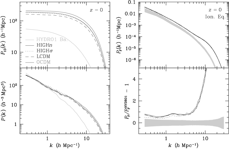
Figure 5.25: Mass PS’s of baryons and dark matter and flux power spectra of simulated Ly$\alpha$ forests for five cosmological models at $z=0$. The upper left panel shows one-dimensional mass PS’s, and the lower panel three-dimensional mass PS’s. The upper right panel shows flux PS’s, and the lower panel residuals of flux PS’s with respect to the flux PS of Ly$\alpha$ forests generated with baryons in ionization equilibrium from HYDRO1 (light grey lines and bands). All others flux PS’s are from $N$-body simulations using the method DI.

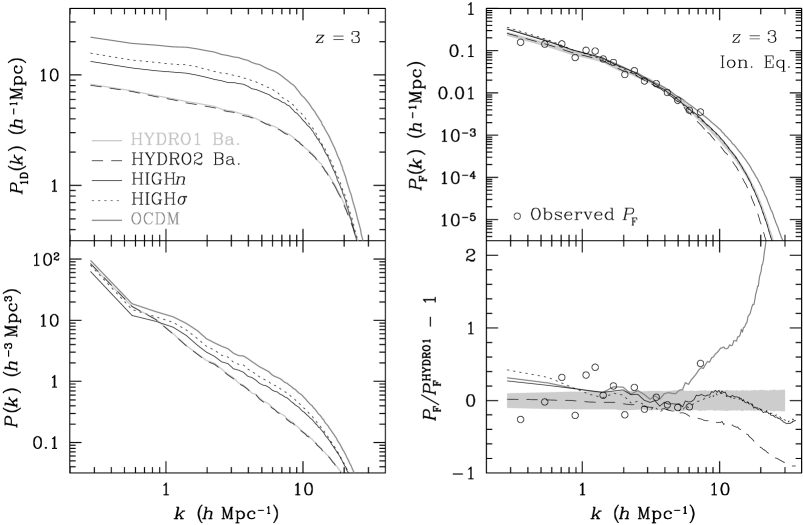
Figure 5.26: The same as Fig. 5.25 except that dark-matter-based PS’s from the simulation LCDM is replaced by baryon-based PS’s from HYDRO2, and that all PS’s are at $z=3$. The observed flux PS is measured from 27 segments of Ly$\alpha$ forests between $z=2.9$ and $3.1$.

It is seen that the flux PS of the 27 Ly$\alpha$ forest segments is roughly matched by all the simulations at $z=3$. The scatter of the observed flux PS is too large to be useful for determining cosmological parameters because of the small size of the sample. But with a much larger number of Ly$\alpha$ forests, it is possible to reduce the sample variance error of the flux PS and place meaningful constraints on cosmology.

Chapter 6 Inverting the Ly$\boldsymbol{\alpha}$ Forest

There are two ways of obtaining density statistics from the Ly$\alpha$ forest. One is to measure flux statistics and then map them into density statistics. The other is to measure statistics of densities inverted from the Ly$\alpha$ forest. As discussed in previous chapters, pseudo-hydro techniques are good approximations at $z=3$, but they still require precise calibrations using hydrodynamical simulations. On the other hand, it is not practical to search the parameter space using hydrodynamical simulations that incorporate all important astrophysical processes. Therefore, it is worthwhile exploring methods of inverting the Ly$\alpha$ forest.

Baryon densities $\rho_{\mathrm{b}}$ and mass densities $\rho$ may be extracted from transmitted fluxes $F$ of Ly$\alpha$ forests using the same equation that is used in the pseudo-hydro technique DE, i.e.

$$F=e^{-\tau}\simeq e^{-A(\rho_{\mathrm{b}}/\bar{\rho}_{\rm b})^{\gamma}}\simeq e^{-A(\rho/\bar{\rho})^{\gamma}}.$$ (6.1)

More accurately, one should also include ionization equilibrium, thermal broadening, etc. A question may be raised here: given the uncertainty of pseudo-hydro techniques, what can be gained by inverting the Ly$\alpha$ forest using equation (6.1)? It is seen in Figs. 5.9 and 5.11 that the lack of temperature information is the major source of error for pseudo-hydro techniques. Whereas, one could determine temperatures of observed Ly$\alpha$ forests from line profiles and obtain relatively accurate baryon densities. Then, the mass PS of baryons on large scales can be used to constrain cosmology.

When the density is high enough, the spectrum is saturated, i.e. $F\simeq 0$. With noises and uncertainties in the spectrum, a direct inversion using equation (6.1) is very unreliable in saturated regions. Despite the difficulty, methods of direct inversion are systematically developed, for example, with Lucy’s method by Nusser & Haehnelt (1999), and with Bayesian method for a three-dimensional inversion by Pichon et al. (2001). One may also use higher order lines to recover the optical depth and the underlying density (Cowie & Songaila 1998; Aguirre, Schaye & Theuns 2002), even though the contamination by lower order lines needs to be carefully removed. Once LOS densities are obtained, many statistics, such as the one-dimensional mass PS, can be measured.

The saturation problem is avoided if one maps the mass PS directly from the flux PS of the Ly$\alpha$ forest without an inversion (Croft et al. 1998, 1999, 2002). However, a close examination of the Fourier transform of equation (6.1) shows that Fourier modes on different scales are mixed by the nonlinear density–flux relation (see Section 6.3). The mixing depends on the underlying density field, and it is hard to predict analytically.

If the inversion is necessary, a proper treatment in saturated regions has to be developed. In many physical systems, sizes are often correlated with other quantities such as masses and densities. For example, more massive stars or dark matter halos have larger sizes, but lower mean densities (Binney & Merrifield 1998; Navarro, Frenk & White 1996). One may expect a similar trend for the saturated Ly$\alpha$ absorption. On the contrary, the mean density is found to increase with the width of saturation. This is due to the fact that the IGM is very diffuse and far from virialization, while the other objects mentioned above are the opposite.

In this chapter, densities are expressed in units of their corresponding cosmic mean densities, and the subscript for LOS wavenumber is dropped for convenience.

6.1 Correlation between the Mean Density and Width of Saturated Ly$\boldsymbol{\alpha}$ Absorptions

Neglecting the probability that two physically separate absorption systems fall in the same redshift coordinate, one can associate a saturated absorption in the Ly$\alpha$ forest with a single high density region. If I assume further that there is no substructure present, and the IGM evolves more or less the same way everywhere, then the size of the saturated region has to be tightly correlated with its mean density (see also Schaye 2001). In reality, the neglected elements above and uncertainties elsewhere will introduce a spread to the correlation.

6.1.1 Simulations

Figs. 5.10, 5.19, and additional tests at $z=4$ demonstrate that pseudo-hydro techniques work very well at $z\gtrsim 2$. Therefore, I choose $N$-body simulations to investigate the relation between the mean density and width of saturated Ly$\alpha$ absorptions.

A standard particle-particle-particle-mesh (P³M, Hockney & Eastwood 1981) code developed by Jing & Fang (1994) is used to evolve 128³ dark matter particles in a cubic box of 12.8 $h^{-1}$Mpc (comoving) each side. The initial PS is given by the fitting formula from Bardeen et al. (1986). The model parameters are listed in Table 6.1. All the models start from $z=15$ and stop at $z=3$ in 950 steps.

Table 6.1: Parameters of the $N$-body simulations.

Model	$\Omega$	$\Omega_{\Lambda}$	$h$	$\Gamma^{\ a}$	$\sigma_{\mathrm{8}}$
LCDM	0.3	0.7	0.7	0.21	0.85
OCDM	0.3	0	0.7	0.21	0.85
SCDM	1.0	0	0.5	0.5	0.67
TCDM	1.0	0	0.5	0.25	0.60

• $\Gamma$ is the shape parameter of the PS.

The parameter $A$ in equation (6.1) is chosen to fit the mean flux equation (5.4). I extrapolate the mean flux up to $z=4.5$, which is not critical to the analysis in Section 6.1.2 but is, nevertheless, supported by simulations (Riediger et al. 1998). The constant $\gamma$ in equation (6.1) is set to $1.6$ since it is the best fit in Fig. 5.14. Four samples of the Ly$\alpha$ forest are shown in Fig. 6.1. They are drawn from the LCDM simulation at $z=3$. The corresponding LOS densities are plotted along with the fluxes. It is evident that most of the Ly$\alpha$ lines arise where $\rho\lesssim 10$.

Figure 6.1: Simulated Ly$\alpha$ forests and LOS densities from the LCDM model at $z=3$. The solid lines are the flux $F$, the dashed lines are the matter density $\rho$, the dotted lines are the recovered density, and the horizontal dash-dotted lines indicate the threshold flux level $\eta=0.03$ (see Section 6.2) in the upper 2 panels, and $\eta=0.10$ in the lower 2 panels.

6.1.2 The Correlation

I define the width $w$ of the saturation as the distance between the two points that bracket the absorption at a given threshold flux level $\eta$. In other words, it is the width of a region in which $F<\eta$. Since the flux $F$ in the saturated region is dominated by noise, one should set the threshold above the noise level. That is why I have not added any noise in the simulations: noise outside the saturation can be routinely dealt with, while noise in the saturation, being below the threshold, does not matter. Within a reasonable range of spectral quality, I choose the threshold $\eta=0.03$ and $0.10$ for tests below.

Figure 6.2: The correlation between the mean density $\bar{\rho}_{\rm a}$ and width $w$ of saturated regions in the Ly$\alpha$ forest. The trend lines fit the data well beyond $2\ h^{-1}$Mpc, even though they are obtained by fitting only the data with $w\leq 2\ h^{-1}$Mpc. The data above $0.3\ h^{-1}$Mpc are binned in logarithmic intervals for readability. Similar treatments apply to Figs. 6.4, 6.5, 6.6, and 6.9 as well.

Once the width is determined, the mean density $\bar{\rho}_{\rm a}$ can be readily calculated from the corresponding LOS density field. Since the density and the flux are assigned only on grid points, interpolation is needed to find $w$ and $\bar{\rho}_{\rm a}$. Fig. 6.2 shows the scaling relation for the LCDM model at $z=3$. It clearly demonstrates that $\bar{\rho}_{\rm a}$ increases with $w$. Furthermore, the correlation is reasonably tight for narrow saturations. Note that the trend lines are obtained by fitting only the data with $w\leq 2\ h^{-1}$Mpc, because wider saturations are very rare as compared to the rest.

The $\bar{\rho}_{\rm a}$–$w$ relation is well fitted by

$$\bar{\rho}_{\rm a}=\rho_{\mathrm{0}}+a\ (w/h^{-1}\mbox{Mpc})^{b}.$$ (6.2)

The term $\rho_{\mathrm{0}}$ sets a baseline for the scaling, because the matter density is non-vanishing even if there is no saturation. The parameter $a$ is a scaling coefficient, which reflects the overall amplitude of the density fluctuation, and the exponent $b$ is more or less determined by the nature of hierarchical clustering. The width $w$ is in units of $h^{-1}$Mpc. Table 6.2 lists the values for the LCDM model at $z=3$ and $4.5$.

Table 6.2: Parameters in the fitting $\bar{\rho}_{\rm a}=\rho_{\mathrm{0}}+a\ (w/h^{-1}\mbox{Mpc})^{b}$ for the LCDM model.

$z$	$\eta$	$\rho_{\mathrm{0}}$	a	b
3	0.03	1.93	3.85	0.545
	0.10	1.39	3.39	0.564
4.5	0.03	0.11	2.78	0.455
	0.10	0.24	2.04	0.556

The reason why $\rho_{\mathrm{0}}$ decreases with redshift is that the universe is more uniform early on, so that even low density regions have to absorb a substantial amount of Ly$\alpha$ flux to produce the low mean flux. This is possible because the neutral fraction of the IGM at $z=4.5$ is higher than that at $z=3$. As the universe evolves, density fluctuations grows stronger and stronger, and the scaling coefficient $a$ becomes larger and larger. The exponent $b$ has changed little over $z=3$–$4.5$. The parameters also show a dependence on the threshold flux $\eta$, because $\eta$ sets the threshold density $\rho_{\eta}$, above which the $\bar{\rho}_{\rm a}$–$w$ relation is explored.

Fig. 6.3 shows the evolution of the $\bar{\rho}_{\rm a}$–$w$ relation for the four models. The difference between models is mostly due to the amplitude of fluctuations—in other words, the PS.

Figure 6.3: Best-fittings of the $\bar{\rho}_{\rm a}$–$w$ relation for the four models at $z=3$–$4.5$. The threshold $\eta=0.03$. The parameters are obtained by fitting the saturations with $w\leq 2\ h^{-1}$Mpc.

6.1.3 A Simple Model

The $\bar{\rho}_{\rm a}$–$w$ relation is analogous—but not completely equivalent—to the curve of growth (e.g. Press & Rybicki 1993), which studies the correlation between the H i column density $N_{\rm HI}$ and the equivalent width $W$ of Ly$\alpha$ absorptions. The similarity is as follows. The width $w$ is approximately the same as $W$, and the mean matter density $\bar{\rho}_{\rm a}$ is proportional to $w^{-1}N_{\rm HI}$ if $\rho\propto\rho_{\mathrm{b}}$ holds true. Since $N_{\rm HI}\propto W$ at small values of $W$, it is not surprising to see $\bar{\rho}_{\rm a}$ grow slowly, i.e. $\mathrm{d}\ln\bar{\rho}_{\rm a}/\mathrm{d}\ln w\sim 0$, for small $w$.

On the other hand, the $\bar{\rho}_{\rm a}$–$w$ relation addresses saturated absorptions where, according to the curve-of-growth analysis, $W$ is almost a constant independent of the H i column density. Therefore, $\bar{\rho}_{\rm a}$ would have risen steeply against $w$, i.e. $b\gg 1$. This apparent inconsistency arises from the cosmological context, because the width $w$ is determined not only by $N_{\rm HI}$ but also by the physical extent of the (relatively) dense region through Hubble expansion and peculiar velocities.

Although it is not obvious why the exponent $b$ is less than unity, I can make an order-of-magnitude estimate using the density profile $\rho(r)\propto r^{-1}$ from a spherical self-similar infall. I modify the profile to avoid the singularity at $r=0$ by adding a smoothing length $\epsilon$, so that $\rho(r)\propto(r^{2}+\epsilon^{2})^{-1/2}$. The mean density within the radius $R$, at which $\rho=\rho_{\eta}$, is

$$\bar{\rho}_{\rm a}(R) = \frac{3}{R^{3}}\int_{0}^{R}\rho(r)r^{2}dr=\frac{3\rho_{\eta}\sqrt{R^{2}+\epsilon^{2}}}{2R^{3}}\times$$

$$\left[R\sqrt{R^{2}+\epsilon^{2}}+\epsilon^{2}\log\left(\frac{\epsilon}{R+\sqrt{R^{2}+\epsilon^{2}}}\right)\right].$$

From equation (6.1.3), one gets an estimate $b\sim\mathrm{d}\ln\bar{\rho}_{\rm a}/\mathrm{d}\ln R=0.39,\ 0.42$, and $0.43$ for $\epsilon=0.2,\ 0.3$, and $0.4\ h^{-1}$Mpc respectively at $R=2\ h^{-1}$Mpc. The same quantity for the $\bar{\rho}_{\rm a}$–$w$ relation is $\mathrm{d}\ln\bar{\rho}_{\rm a}/\mathrm{d}\ln w=0.41$, where I have used the parameters of the LCDM model at $z=3$ with $\eta=0.03$ (see Table 6.2). It should be emphasized that the profile $\rho(r)\propto r^{-1}$ is not quite justified for the IGM at $z=3$, and without any modification, it gives the same mean density within the boundary $\rho=\rho_{\eta}$ regardless the size of the system, i.e. $b=0$. Therefore, equation (6.1.3) is not expected to give a good approximation of the $\bar{\rho}_{\rm a}$–$w$ relation.

6.2 Inversion with A Gaussian Density Profile

If the flux level is above the threshold, equation (6.1) can be used to find the density. When it is below the threshold, one must provide a density profile that matches $\bar{\rho}_{\rm a}(w)$ and $\rho_{\eta}$ to fill in the missing information in the saturation.

While the density profile is worth studying in its own right, I simply choose the Gaussian profile

$$\rho(s)=\frac{B}{\sigma\sqrt{2\pi}}\exp\left[-\frac{1}{2}\bigl{(}\frac{s-s_{\mathrm{0}}}{\sigma}\bigr{)}^{2}\right],$$ (6.4)

where $s$ is the coordinate in redshift space, $s_{\mathrm{0}}$ is the center of the saturation, and $B$ and $\sigma$ are solved simultaneously from

$$\bar{\rho}_{\rm a}(w) = \frac{1}{w}\int^{s_{\mathrm{0}}+w/2}_{s_{0}-w/2}\rho(s)ds=\frac{B}{w}\mbox{ erf}\Bigl{(}\frac{1}{2\sqrt{2}}\frac{w}{\sigma}\Bigr{)},$$ (6.5)

$$\rho_{\eta} = \rho(s_{\mathrm{0}}\pm w/2)=\frac{B}{\sigma\sqrt{2\pi}}\exp\left[-\frac{1}{8}\bigl{(}\frac{w}{\sigma}\bigr{)}^{2}\right],$$

where erf($x$) is the error function. The Gaussian profile has the advantage that it does not introduce any artificial power on small scales. However, it is arguable that the right amount of small-scale power should be added through the profile, and so a more realistic profile may be needed.

Figure 6.4: One-dimensional mass PS’s of original densities and inverted densities in redshift space. Circles include all LOS’s from the N-body simulation, and the dashed line contains only the ones that have a maximum width of saturation $w_{\mathrm{M}}<1\ h^{-1}$Mpc. The recovered densities are inverted from fluxes with thresholds $\eta=0.03$ (solid line) and $\eta=0.1$ (dotted line). The error bars are 1$\sigma$ dispersions among 610 groups, each of which consists of 20 LOS’s. The error bars of the recovered densities, which are not plotted, are comparable to that of the original densities.

The recovered LOS densities with $\eta=0.03$ and $\eta=0.10$ are shown along with the four original LOS densities and fluxes in Fig. 6.1. Since a universal density profile is employed in the inversion, the recovered densities do not necessarily match the original densities.

To assess the statistical quality of the inversion, I plot in Fig. 6.4 the original and recovered mass PS’s of the LCDM model with different flux thresholds. Other models are shown in Fig. 6.5. The recovered PS has good agreement with the original PS on large scales ($k\lesssim 3\ h$ Mpc^-1), but it is underestimated on smaller scales, where the Gaussian profile essentially has no power. The signal to noise ratio, or the threshold flux, has little influence on large scales, but a low noise level does slightly improve the recovery on small scales.

Figure 6.5: The same as Fig. 6.4, but for OCDM, SCDM, and TCDM models.

Figure 6.6: The same as Fig. 6.4, except that the fluxes are drawn from the LCDM simulation, while the densities are recovered with $\bar{\rho}_{\rm a}$–$w$ relations from OCDM and TCDM simulations.

For comparison, I show in Figs. 6.4 and 6.5 the original PS of the LOS densities that have a maximum width of saturation $w_{\mathrm{M}}<1\ h^{-1}$Mpc. This is equivalent to removing—or giving less weight to—the saturated regions when one measures the PS. It is seen that the saturated regions are very important to scales $\gtrsim 2\ h^{-1}$Mpc, while the unsaturated regions give a good estimate of the small-scale power. Thus one may improve the recovery of PS as follows. First, invert the Ly$\alpha$ forest with equation (6.1) and the $\bar{\rho}_{\rm a}$–$w$ relation. Second, do the inversion after removing the saturated regions. Finally, the best-estimate of the PS is just the common envelope of the PS’s of the two recovered densities.

Fig. 6.3 indicates that the $\bar{\rho}_{\rm a}$–$w$ relation varies from model to model. Thus it is necessary to check if the recovery is sensitive to $\bar{\rho}_{\rm a}(w)$—in other words, if it is model dependent. In Fig. 6.6 I plot the PS’s of LCDM densities recovered with $\bar{\rho}_{\rm a,O}(w)$ and $\bar{\rho}_{\rm a,T}(w)$ from OCDM and tilted cold dark matter (TCDM) models respectively. It seems that by boosting $\bar{\rho}_{\rm a}(w)$ a small amount [$\bar{\rho}_{\rm a,T}(w)$ lies a little higher than $\bar{\rho}_{\rm a,L}(w)$], one gets even better estimate of the PS on small scales. However, lowering $\bar{\rho}_{\rm a}(w)$ could underestimate the power by a factor of 2 on large scales, and even more on small scales. The effect of this model dependence could be reduced with the constraint on small scales, since it is possible to recover the small-scale power well by removing the saturations.

Fig. 6.7 tests a different statistics—the one-point distribution function for the LCDM model. It is evident that the Gaussian profile leads to a drop of the probability at high densities. In other words, it statistically reduces the heights of density peaks.

Figure 6.7: The one-point distribution function of inverted densities (filled circles) and that of the original densities (open squares).

6.3 Mapping the Power Spectra

It seems that the inversion is no longer needed at least for determining the mass PS if one establishes a direct mapping between the flux and the mass PS’s (Croft et al. 2002). It is shown that given a set of cosmological parameters, there is a statistical mapping, which reliably recovers the mass PS from the flux PS (Gnedin & Hamilton 2002), even though the mapping is model dependent.

Figure 6.8: Three-dimensional mass PS’s of the LCDM model at $z=3$. The dashed lines are the real-space PS’s, the dotted lines are the redshift-space PS’s averaged over solid angles, and the thin solid line is the initial PS (at $z=15$) evolved to $z=3$ by linear theory. The thin dashed line and the thin dotted line are from an additional simulation with the same parameters as the LCDM model except that the box is 51.2 $h^{-1}$Mpc each side.

The physical links between the three-dimensional linear mass PS $P_{\mathrm{L}}(k)$ and the flux PS can be summarized by the flowchart:

$$P_{\mathrm{L}}(k)\longrightarrow P_{\mathrm{NL}}(k)\longrightarrow P_{\mathrm{NL}}^{S}(\mathbf{k})\longrightarrow P^{S}_{\rm 1D}(k)\buildrel d^{2}(k)\over{\longrightarrow}P_{\mathrm{F}}(k),$$

where $P_{\mathrm{NL}}(k)$ is the three-dimensional nonlinear mass PS (Peacock & Dodds 1996; Taylor & Hamilton 1996), $P_{\mathrm{NL}}^{S}(\mathbf{k})$ is $P_{\mathrm{NL}}(k)$ in redshift-space (Kaiser 1987; Peacock 1999; Zhan & Fang 2003), and $d^{2}(k)=P_{\mathrm{F}}(k)/P^{S}_{\rm 1D}(k)$. Note that $P_{\mathrm{NL}}^{S}(\mathbf{k})$ is anisotropic. I show in Fig. 6.8 that the nonlinear evolution and redshift distortion are already significant at $z=3$. The fact that the departure from linear evolution is very similar in both large and small box simulations indicates that such departure is real, and the cosmic density field has already gone nonlinear below 10 $h^{-1}$Mpc ($k>0.6$ $h$ Mpc^-1) at $z=3$ (see also Pichon et al. 2001; Zhan et al. 2001). The angularly averaged three-dimensional PS $P_{\mathrm{NL}}^{S}(k)$, i.e. the monopole, does not give a complete view of the difference between the real-space PS and redshift-space PS, but it does show that peculiar velocities boost the power on large scales and reduce it substantially on small scales as seen in Fig. 5.7. A two-dimensional projection of $P_{\mathrm{NL}}^{S}(\mathbf{k})$ can be found in Peacock et al. (2001).

In contrast, the mapping in Croft et al. (2002) follows a simplified path:

$$P_{\mathrm{L}}(k)\longrightarrow P_{\mathrm{1D,L}}(k)\buildrel b^{2}(k)\over{\longrightarrow}P_{\mathrm{F}}(k),$$

where $P_{\mathrm{1D,L}}(k)=(2\pi)^{-1}\int_{k}^{\infty}P_{\mathrm{L}}(y)ydy$, and $b^{2}(k)=P_{\mathrm{F}}(k)/P_{\mathrm{1D,L}}(k)$. Given a one-dimensional density field in redshift space at $z=3$, one can only measure $P^{S}_{\rm 1D}(k)$, and so $P_{\mathrm{1D,L}}(k)$ is not observable unless the density field is linear on all scales and no peculiar velocity is present. In other words, $P^{S}_{\rm 1D}(k)$ is directly connected to $P_{\mathrm{F}}(k)$, while $P_{\mathrm{1D,L}}(k)$ is not.

Around the cosmic mean matter density, i.e. $|\delta|\ll 1$, equation (6.1) is approximately

$$F(s)\simeq e^{-A}-A\gamma e^{-A}\delta(s),$$ (6.6)

where I have included the dependence on the redshift coordinate $s$ explicitly. It is seen in the linearized equation (6.6) that the Fourier modes of the flux are proportional to those of the overdensity when $k\neq 0$. Hence, the flux PS is proportional to the mass PS

$$P_{\mathrm{F}}(k)\simeq A^{2}\gamma^{2}e^{-2A}P^{S}_{\rm 1D}(k),\quad k\neq 0.$$ (6.7)

Caution should be taken when using equation (6.6), because it is valid only if one smoothes the Ly$\alpha$ forest over large scales (see, for example, Zhan et al. 2001; Zhan & Fang 2002).

It is obvious from equation (6.1) and Fig. 6.1 that the condition $|\delta(s)|\ll 1$ is not satisfied when $F\simeq 1$ or $F\simeq 0$. Therefore, one has to include higher order terms of $\delta(s)$. Taking the simplest case, in which $\delta(s)=\sin(k_{\mathrm{0}}s)$ and only $\delta^{2}(s)$ term is added to equation (6.6), one immediately finds that $P_{\mathrm{F}}(k)$ contains spurious power on the mode $2k_{\mathrm{0}}$ that $P^{S}_{\rm 1D}(k)$ does not contain. In general, the nonlinear density–flux relation distorts, spreads, and mixes power in the cosmic density field over different scales in the flux PS. I have not focused other sources of distortion such as linear filtering (Gnedin & Hui 1998), line profile (see Gray 1992), and instrumentation, since they are well studied in the literature.

Figure 6.9: The ratio $b(k)=\sqrt{P_{\mathrm{F}}(k)/P_{\mathrm{1D,L}}(k)}$ (upper panel) and $d(k)=\sqrt{P_{\mathrm{F}}(k)/P^{S}_{\rm 1D}(k)}$ (lower panel). The Ly$\alpha$ forests are divided into groups, each of which consists of 20 LOS’s. The PS’s are averaged within each group except $P_{\mathrm{1D,L}}(k)$, which is theoretical. The error bars of the LCDM model are 1$\sigma$ dispersions among 610 groups. Error bars of other models are comparable to that of the LCDM model.

Fig. 6.9 shows the ratios $b(k)$ and $d(k)$. The dispersion in $d(k)$ is larger than that of $b(k)$, because both $P_{\mathrm{F}}(k)$ and $P^{S}_{\rm 1D}(k)$ contribute to the dispersion of $d(k)$, while $b(k)$ receives only a single contribution from $P_{\mathrm{F}}(k)$. Even so, the error propagation would cause a large scatter in determining $P_{\mathrm{1D,L}}(k)$ and $P_{\mathrm{L}}(k)$. In fact, the scatter can be large enough that one would not be able to determine the cosmological model based only on the recovered $P_{\mathrm{L}}(k)$. On the other hand, the model dependence of $b(k)$ is strong enough, so that one may have to assume a cosmological model to recover the mass PS from the flux PS. The difference among the models is not solely due to $\sigma_{\mathrm{8}}$. For example, the standard cold dark matter (SCDM) model has a slightly higher $\sigma_{\mathrm{8}}$ than the TCDM model, so one would expect $b(k)$ of the SCDM model to have the same shape as that of the TCDM model. This is not observed in Fig. 6.9, however. It is also evident from the behavior of $b(k)$ and $d(k)$ that the PS of the underlying density field $P^{S}_{\rm 1D}(k)$ is significantly lower than the linear mass PS $P_{\mathrm{1D,L}}(k)$ on scales $k>0.02$ (km s^-1)^-1. This is due mostly to peculiar velocities, or redshift distortion.

Chapter 7 Conclusions

I have investigated the covariance of the one-dimensional mass PS for both GRFs and simulated density fields. The nonlinear evolution and non-Gaussianity of the cosmic density field on small scales (see also Zhan et al. 2001; Smith et al. 2003; Zaldarriaga et al. 2003; Zhan 2003) have caused correlations between the fluctuations on different scales and increased the cosmic variance of the one-dimensional mass PS. Because of this, a large number of LOS’s are needed to accurately measure the one-dimensional mass PS and recover the three-dimensional mass PS.

The length of LOS’s introduces a window function in the LOS direction, which mixes neighboring Fourier modes in the cosmic density field. Fig. 4.8 has demonstrated for simulations that the length of LOS’s does affect the covariance of the one-dimensional mass PS. The covariance of the observed one-dimensional mass PS will receive a significant contribution from this effect, because in practice the length of LOS’s suitable for study is always much less than the size of the observable universe [see equation (3.11)].

One may reduce the cosmic variance by binning independent Fourier modes. However, since the modes of the cosmic density field are strongly correlated, binning will be less effective in reducing the sample variance error. On the other hand, the non-Gaussian behavior of the covariance provides important information of the field such as the trispectrum.

Using hydrodynamical simulations and $N$-body simulations, I find that pseudo-hydro techniques are able to reproduce the flux and flux PS that are obtained using the full-hydro method at $z\gtrsim 2$. There is also a good match between observed and simulated flux statistics such as the flux PS and its covariance at $z=3$.

The accuracy of pseudo-hydro techniques does not seem to be high enough for determining cosmology at percent level. One needs to precisely calibrate pseudo-hydro techniques with hydrodynamical simulations. Moreover, it is better to constrain cosmology using the flux PS on scales above a few $h^{-1}$Mpc in order to reduce the uncertainties caused by the IGM temperature and thermal broadening. At low redshift, the shock-heated WHIM has greatly altered the temperature–density relation of the IGM, so that fluctuations in the Ly$\alpha$ flux are strongly suppressed by thermal broadening. As a result, pseudo-hydro techniques overpredict the flux PS at low redshift.

The transform from density to flux quenches fluctuations by orders of magnitude and leads to near-Gaussian Ly$\alpha$ fluxes. Hence, the variance of the flux PS is much less than that of the one-dimensional mass PS. In other words, one can measure the flux PS to a high precision with a relatively small number of LOS’s, but the underlying mass PS cannot be determined as precisely as the flux PS. Attempts to recover the three-dimensional mass PS should take into account the sample variance error of the one-dimensional mass PS.

It is possible to invert the Ly$\alpha$ forest and measure statistics of one-dimensional density fields directly. I provide a scaling relation between the mean matter density $\bar{\rho}_{\rm a}$ and the width of saturated Ly$\alpha$ absorptions $w$, which helps invert saturated Ly$\alpha$ absorptions. The inversion with the $\bar{\rho}_{\rm a}$–$w$ relation is able to recover the redshift-space one-dimensional mass PS fairly well on scales above $2\ h^{-1}$Mpc, but it underestimates the power on small scales due to the use of the Gaussian profile. An improvement is suggested based on the observation that the small-scale one-dimensional mass PS can be better recovered if saturated absorptions are removed. Thus, by combining both the $\bar{\rho}_{\rm a}$–$w$ inversion and the result after removing saturated absorptions, one could get a good estimate of the one-dimensional mass PS over a wide range of scales.

The $\bar{\rho}_{\rm a}$–$w$ relation provides an important constraint to the inversion of the Ly$\alpha$ forest. To incorporate it in any inversion scheme, one needs to determine the $\bar{\rho}_{\rm a}$–$w$ relation according to spectral resolution and noise. The threshold flux can be conveniently set to a small value above the noise level. The recovered redshift-space one-dimensional mass PS is not very sensitive to the $\bar{\rho}_{\rm a}$–$w$ relation on large scales. However, one would greatly underestimate the large-scale one-dimensional mass PS if saturated regions were excluded from the sample.

As seen in Chapters 4 and 5, one-dimensional density fields have a large cosmic variance in their PS due to non-Gaussianity. Nevertheless, this variance can be reduced by a large number of LOS’s. With thousands of Ly$\alpha$ forests from QSO surveys, it is possible to subdue the variance to a few percent level, and the Ly$\alpha$ forest may eventually become comparable to other fields of precision cosmology such as the CMB and weak lensing.

References

- Aguirre, Schaye & Theuns (2002) Aguirre, A., Schaye, J., & Theuns, T. 2002, Astrophys. J., 576, 1
- Bardeen et al. (1986) Bardeen, J. M., Bond, J. R., Kaiser, N., & Szalay, A. S. 1986, Astrophys. J., 304, 15
- Baugh & Efstathiou (1993) Baugh, C. M., & Efstathiou, G. 1993, Mon. Not. R. Astron. Soc., 265, 145
- Bechtold (1994) Bechtold, J. 1994, Astrophys. J. Supp., 91, 1
- Becker et al. (2001) Becker, R. H. et al. 2001, Astron. J., 122, 2850
- Benson et al. (2000) Benson, A. J., Cole, S., Frenk, C. S., Baugh, C. M., & Lacey, C. G. 2000, Mon. Not. R. Astron. Soc., 311, 793
- Bertschinger (2001) Bertschinger, E. 2001, Astrophys. J. Supp., 137, 1
- Bi & Davidsen (1997) Bi, H. G., & Davidsen, A. F. 1997, Astrophys. J., 479, 523
- Binney & Merrifield (1998) Binney, J., & Merrifield, M. 1998, Galactic Astronomy, Princeton Univ. Press, Princeton, NJ, p. 110
- Boyle et al. (2000) Boyle, B. J., Shanks, T., Croom, S. M., Smith, R. J., Miller, L., Loaring, N., & Heymans, C. 2000, Mon. Not. R. Astron. Soc., 317, 1014
- Bryan et al. (1999) Bryan, G. L., Machacek, M., Anninos, P., & Norman, M. L. 1999, Astrophys. J., 517, 13
- Cen et al. (1994) Cen, R., Miralda-Escudé, J., Ostriker, J. P., & Rauch, M. 1994, Astrophys. J. Lett., 437, L9
- Colless et al. (2001) Colless, M. et al. 2001, Mon. Not. R. Astron. Soc., 328, 1039
- Cooray & Hu (2001) Cooray, A., & Hu, W. 2001, Astrophys. J., 554, 56
- Cowie & Songaila (1998) Cowie, L. L., & Songaila, A. 1998, Nature, 394, 44
- Croft et al. (2002) Croft, R. A. C., Weinberg, D. H., Bolte, M., Burles, S., Hernquist, L., Katz, N., Kirkman, D., & Tytler, D. 2002, Astrophys. J., 581, 20
- Croft et al. (1998) Croft, R. A. C., Weinberg, D. H., Katz, N., & Hernquist, L. 1998, Astrophys. J., 495, 44
- Croft et al. (1999) Croft, R. A. C., Weinberg, D. H., Pettini, M., Hernquist, L., & Katz, N. 1999, Astrophys. J., 520, 1
- Davé et al. (2001) Davé, R., Cen, R., Ostriker, J. P., Bryan, G. L., Hernquist, L., Katz, N., Weinberg, D. H., Norman, M. L., & O’Shea, B. 2001, Astrophys. J., 552, 473
- Davé, Dubinski & Hernquist (1997) Davé, R., Dubinski, J., & Hernquist, L. 1997, New Astron., 2, 277
- Davé et al. (1999) Davé, R., Hernquist, L., Katz, N., & Weinberg, D. H. 1999, Astrophys. J., 511, 521
- Davé et al. (1997) Davé, R., Hernquist, L., Weinberg, D. H., & Katz, N. 1997, Astrophys. J., 477, 21
- Davé & Tripp (2001) Davé, R., & Tripp, T. M. 2001, Astrophys. J., 553, 528
- Dekel & Lahav (1999) Dekel, A., & Lahav, O. 1999, Astrophys. J., 520, 24
- Dekel & Silk (1986) Dekel, A., & Silk, J. 1986, Astrophys. J., 303, 39
- Dodelson et al. (2002) Dodelson, S. et al. 2002, Astrophys. J., 572, 140
- Dobrzycki & Bechtold (1996) Dobrzycki, A. & Bechtold, J. 1996, Astrophys. J., 457, 102
- Fan et al. (2001) Fan, X. et al. 2001, Astron. J., 122, 2833
- Fan et al. (2003) Fan, X. et al. 2003, Astron. J., 125, 1649
- Fang & Feng (2000) Fang, L.-Z., & Feng, L.-L. 2000, Astrophys. J., 539, 5
- Feldman, Kaiser & Peacock (1994) Feldman, H. A., Kaiser, N., & Peacock, J. A. 1994, Astrophys. J., 426, 23
- Feng & Fang (2000) Feng, L.-L., & Fang, L.-Z. 2000, Astrophys. J., 535, 519
- Feng, Pando & Fang (2001) Feng, L.-L., Pando, J., & Fang, L.-Z. 2001, Astrophys. J., 555, 74
- Fisher et al. (1996) Fisher, K. B., Bahcal, J. N., Kirhakos, S., & Schneider, D. P. 1996, Astrophys. J., 468, 469
- Fisher et al. (1993) Fisher, K. B., Davis, M., Strauss, M. A., Yahil, A., & Huchra, J. P. 1993, Astrophys. J., 402, 42
- Gaztanaga & Frieman (1994) Gaztanaga, E., & Frieman, J. A. 1994, Astrophys. J. Lett., 437, L13
- Gnedin & Hamilton (2002) Gnedin, N. Y., & Hamilton, A. J. S. 2002, Mon. Not. R. Astron. Soc., 334, 107
- Gnedin & Hui (1998) Gnedin, N. Y., & Hui, L. 1998, Mon. Not. R. Astron. Soc., 296, 44
- Gray (1992) Gray, D. 1992, The Observation and Analysis of Stellar Photospheres, Cambridge Univ. Press, New York
- Gunn & Peterson (1965) Gunn, J. E., & Peterson, B. A. 1965, Astrophys. J., 142, 1633
- Haardt & Madau (1996) Haardt, F., & Madau, P. 1996, Astrophys. J., 461, 20
- Hernquist et al. (1996) Hernquist, L., Katz, N., Weinberg, D. H., & Miralda-Escudé, J. 1996, Astrophys. J. Lett., 457, L51
- Hockney & Eastwood (1981) Hockney, R. W., & Eastwood, J. W. 1981, Computer Simulation Using Particles, McGraw-Hill, New York
- Hubble (1934) Hubble, E. 1934, Astrophys. J., 79, 8
- Huchra et al. (1990) Huchra, J. P., Geller, M. J., de Lapparent, V., & Corwin, H. G., Jr. 1990, Astrophys. J. Supp., 72, 433
- Hui (1999) Hui, L. 1999, Astrophys. J., 516, 519
- Hui et al. (2001) Hui, L., Burles, S., Seljak, U., Rutledge, R. E., Magnier, E., & Tytler, D. 2001, Astrophys. J., 552, 15
- Hui & Gnedin (1997) Hui, L., & Gnedin, N. Y. 1997, Mon. Not. R. Astron. Soc., 292, 27
- Iovino & Shaver (1988) Iovino, A., & Shaver, P. A. 1988, Astrophys. J. Lett., 330, L13
- Jeans (1928) Jeans, J. 1928, Astronomy and Cosmogony, Cambridge Univ. Press, Cambridge
- Jing & Fang (1994) Jing, Y. P., & Fang, L.-Z. 1994, Astrophys. J., 432, 438
- Kaiser (1987) Kaiser, N. 1987, Mon. Not. R. Astron. Soc., 227, 1
- Kaiser & Peacock (1991) Kaiser, N., & Peacock, J.A. 1991, Astrophys. J., 379, 482
- Katz, Weinberg & Hernquist (1996) Katz, N., Weinberg, D. H., & Hernquist, L. 1996, Astrophys. J. Supp., 105, 19
- Kauffmann & Haehnelt (2002) Kauffmann, G., & Haehnelt, M. G. 2002, Mon. Not. R. Astron. Soc., 332, 529
- Kauffmann, Nusser & Steinmetz (1997) Kauffmann, G., Nusser, A., & Steinmetz, M. 1997, Mon. Not. R. Astron. Soc., 286, 795
- Kim et al. (2002) Kim, T.-S., Carswell, R. F., Cristiani, S., D’Odorico, S., & Giallongo, E. 2002, Mon. Not. R. Astron. Soc., 335, 555
- Kim et al. (2004) Kim, T.-S., Viel, M., Haehnelt, M. G., Carswell, R. F., & Cristiani, S. 2004, Mon. Not. R. Astron. Soc., 347, 355
- La Franca, Andreani & Cristiani (1998) La Franca, F., Andreani, P., & Cristiani, S. 1998, Astrophys. J., 497, 529
- Lahav et al. (1991) Lahav, O., Rees, M. J., Lilje, P. B., & Primack, J. R. 1991, Mon. Not. R. Astron. Soc., 251, 128
- Lemaître (1934) Lemaître, G. 1934, Proc. Natl. Acad. Sci., 20, 12
- Lin et al. (1996) Lin, H., Kirshner, R. P., Shectman, S. A., Landy, S. D., Oemler, A., Tucker, D. L., & Schechter, P. L. 1996, Astrophys. J., 471, 617
- Lu et al. (1996) Lu, L., Sargent, W. L. W., Womble, D. S., & Takada-Hidai, M. 1996, Astrophys. J., 472, 509
- Lumsden, Heavens & Peacock (1989) Lumsden, S. L., Heavens, A. F., & Peacock, J. A. 1989, Mon. Not. R. Astron. Soc., 238, 293
- Ma & Bertschinger (1995) Ma, C.-P., & Bertschinger, E. 1995, Astrophys. J., 455, 7
- Maddox et al. (1990) Maddox, S. J., Efstathiou, G., Sutherland, W. J., & Loveday, J. 1990, Mon. Not. R. Astron. Soc., 243, 692
- Mandelbaum et al. (2003) Mandelbaum, R., McDonald, P., Seljak, U., & Cen, R. 2003, Mon. Not. R. Astron. Soc., 344, 776
- McDonald (2003) McDonald, P. 2003, Astrophys. J., 585, 34
- McDonald & Miralda-Escudé (1999) McDonald, P., & Miralda-Escudé, J. 1999, Astrophys. J., 518, 24
- McDonald & Miralda-Escudé (2001) McDonald, P., & Miralda-Escudé, J. 2001, Astrophys. J. Lett., 549, L11
- McDonald et al. (2000) McDonald, P., Miralda-Escudé, J., Rauch, M., Sargent, W. L. W., Barlow, T. A., Cen, R., & Ostriker, J. P. 2000, Astrophys. J., 543, 1
- Meiksin & White (1999) Meiksin, A., & White, M. 1999, Mon. Not. R. Astron. Soc., 308, 1179
- Meiksin & White (2004) Meiksin, A., & White, M. 2004, submitted to Mon. Not. R. Astron. Soc., astro-ph/0307289
- Milne (1935) Milne, E. A. 1935, Relativity, Gravitation and World Structure, Clarendon Press, Oxford
- Miralda-Escudé et al. (1996) Miralda-Escudé, J., Cen, R., Ostriker, J. P., & Rauch, M. 1996, Astrophys. J., 471, 582
- Mo & Fang (1993) Mo, H. J., & Fang, L.-Z. 1993, Astrophys. J., 410, 493
- Monaghan & Lattanzio (1985) Monaghan, J. J., & Lattanzio, J. C. 1985, Astron. Astrophys., 149, 135
- Navarro, Frenk & White (1996) Navarro, J. F., Frenk, C. S., & White, S. D. M. 1996, Astrophys. J., 462, 563
- Nusser & Haehnelt (1999) Nusser, A., & Haehnelt, M. 1999, Mon. Not. R. Astron. Soc., 303, 179
- Outram et al. (2003) Outram, P. J., Hoyle, F., Shanks, T., Croom, S. M., Boyle, B. J., Miller, L., Smith, R. J., & Myers, A. D. 2003, Mon. Not. R. Astron. Soc., 342, 483
- Pascarelle et al. (2001) Pascarelle, S. M., Lanzetta, K. M., Chen, H.-W., & Webb, J. K. 2001, Astrophys. J., 560, 101
- Peacock (1991) Peacock, J. A. 1991, Mon. Not. R. Astron. Soc., 253, 1
- Peacock (1999) Peacock, J. A. 1999, Cosmological Physics, Cambridge Univ. Press, Cambridge
- Peacock & Dodds (1996) Peacock J. A. & Dodds S. J. 1996, Mon. Not. R. Astron. Soc. Lett., 280, L19
- Peacock & Smith (2000) Peacock, J. A., & Smith, R. E. 2000, Mon. Not. R. Astron. Soc., 318, 1144
- Peacock et al. (2001) Peacock, J. A. et al. 2001, Nature, 410, 169
- Peebles (1980) Peebles, P. J. E. 1980, The Large Scale Structure of the Universe, Princeton Univ. Press, Princeton
- Peebles (1993) Peebles, P. J. E. 1993, Principles of Physical Cosmology, Princeton Univ. Press, Princeton
- Percival et al. (2001) Percival, W. J. et al. 2001, Mon. Not. R. Astron. Soc., 327, 1297
- Petitjean, Mücket & Kates (1995) Petitjean, P., Mücket, J. P., & Kates, R. E. 1995, Astron. Astrophys. Lett., 295, L9
- Pichon et al. (2001) Pichon, C., Vergely, J. L., Rollinde, E., Colombi, S., & Petitjean, P. 2001, Mon. Not. R. Astron. Soc., 326, 597
- Press & Rybicki (1993) Press, W. H., & Rybicki, G. B. 1993, Astrophys. J., 418, 585
- Rauch (1998) Rauch, M. 1998, Ann. Rev. Astron. Astrophys., 36, 267
- Rauch et al. (1997) Rauch, M. et al. 1997, Astrophys. J., 489, 7
- Riediger, Petitjean & Mücket (1998) Riediger, R., Petitjean, P., & Mücket, J. P. 1998, Astron. Astrophys., 329, 30
- Saunders et al. (2000) Saunders, W. et al. 2000, Mon. Not. R. Astron. Soc., 317, 55
- Schaye (2001) Schaye, J. 2001, Astrophys. J., 559, 507
- Scott et al. (2000) Scott, J., Bechtold, J., Dobrzycki, A., & Kulkarni, V. P. 2000, Astrophys. J. Supp., 130, 67
- Seljak, McDonald & Makarov (2003) Seljak, U., McDonald, P., & Makarov, A. 2003, Mon. Not. R. Astron. Soc. Lett., 342, L79
- Shanks & Boyle (1994) Shanks, T., & Boyle, B. J. 1994, Mon. Not. R. Astron. Soc., 271, 753
- Shanks et al. (1987) Shanks, T., Fong, R., Boyle, B. J., & Peterson, B. A. 1987, Mon. Not. R. Astron. Soc., 227, 739
- Shannon (1949) Shannon, C. E. 1949, Proc. IRE, 37, 10
- Shapley (1934) Shapley, H. 1934, Mon. Not. R. Astron. Soc., 94, 791
- Shaver (1984) Shaver, P. A. 1984, Astron. Astrophys. Lett., 136, L9
- Shectman et al. (1996) Shectman, S. A., Landy, S. D., Oemler, A., Tucker, D. L., Lin, H., Kirshner, R. P., & Schechter, P. L. 1996, Astrophys. J., 470, 172
- Smith et al. (2003) Smith, R. E. et al. 2003, Mon. Not. R. Astron. Soc., 341, 1311
- Somerville et al. (2001) Somerville, R. S., Lemson, G., Sigad, Y., Dekel, A., Kauffmann, G., & White, S. D. M. 2001, Mon. Not. R. Astron. Soc., 320, 289
- Spergel et al. (2003) Spergel, D. N. et al. 2003, Astrophys. J. Supp., 148, 175
- Springel, Yoshida & White (2001) Springel, V., Yoshida, N., & White, S. D. M. 2001, New Astron., 6, 79
- Stoughton et al. (2002) Stoughton, C. et al. 2002, Astron. J., 123, 485
- Taylor & Hamilton (1996) Taylor, A. N., & Hamilton, A. J. S. 1996, Mon. Not. R. Astron. Soc., 282, 767
- Theuns, Leonard & Efstathiou (1998) Theuns, T., Leonard, A., & Efstathiou, G. 1998, Mon. Not. R. Astron. Soc. Lett., 297, L49
- Tyson (1986) Tyson, J. A. 1986, Astron. J., 92, 691
- Unser (2000) Unser, M. 2000, Proc. IEEE, 88, 569
- Verde et al. (2002) Verde, L. et al. 2002, Mon. Not. R. Astron. Soc., 335, 432
- Viel et al. (2004) Viel, M., Haehnelt, M. G., Carswel, R. F., & Kim, T.-S. 2004, submitted to Mon. Not. R. Astron. Soc., astro-ph/0307078
- Viel et al. (2004) Viel, M., Matarrese, S., Heavens, A., Haehnelt, M. G., Kim, T.-S., Springel, V., & Hernquist, L. 2004, Mon. Not. R. Astron. Soc. Lett., 347, L26
- Viel et al. (2002) Viel, M., Matarrese, S., Mo, H. J., Haehnelt, M. G., & Theuns, T. 2002, Mon. Not. R. Astron. Soc., 329, 848
- Viel et al. (2003) Viel, M., Matarrese, S., Theuns, T., Munshi, D., & Wang, Y. 2003, Mon. Not. R. Astron. Soc. Lett., 340, L47
- Weinberg et al. (2004) Weinberg, D. H., Davé, R., Katz, N., & Hernquist, L. 2004, Astrophys. J., 601, 1
- Zaldarriaga, Hui & Tegmark (2001) Zaldarriaga, M., Hui, L., & Tegmark, M. 2001, Astrophys. J., 557, 519
- Zaldarriaga, Scoccimarro & Hui (2003) Zaldarriaga, M., Scoccimarro, R., & Hui, L. 2003, Astrophys. J., 590, 1
- Zhan (2003) Zhan, H. 2003, Mon. Not. R. Astron. Soc., 344, 935
- Zhan & Fang (2002) Zhan, H., & Fang, L.-Z. 2002, Astrophys. J., 566, 9
- Zhan & Fang (2003) Zhan, H., & Fang, L.-Z. 2003, Astrophys. J., 585, 12
- Zhan, Jamkhedkar & Fang (2001) Zhan, H., Jamkhedkar, P., & Fang, L.-Z. 2001, Astrophys. J., 555, 58
- Zhang, Anninos & Norman (1995) Zhang, Y., Anninos, P., & Norman, M. L. 1995, Astrophys. J. Lett., 453, L57
- Zhang et al. (1998) Zhang, Y., Meiksin, A., Anninos, P., & Norman, M. L. 1998, Astrophys. J., 495, 63