On the Hipparcos parallaxes of O stars

We compare the absolute visual magnitude of the majority of bright O stars in the sky as predicted from their spectral type with the absolute magnitude calculated from their apparent magnitude and the Hipparcos parallax. We find that many stars appear to be much fainter than expected, up to five magnitudes. We find no evidence for a correlation between magnitude differences and the stellar rotational velocity as suggested for OB stars by Lamers et al. (1997), whose small sample of stars is partly included in ours. Instead, by means of a simulation we show how these differences arise naturally from the large distances at which O stars are located, and the level of precision of the parallax measurements achieved by Hipparcos. Straightforwardly deriving a distance from the Hipparcos parallax yields reliable results for one or two O stars only. We discuss several types of bias reported in the literature in connection with parallax samples (Lutz-Kelker, Malmquist) and investigate how they affect the O star sample. In addition, we test three absolute magnitude calibrations from the literature (Schmidt-Kaler et al. 1982; Howarth & Prinja 1989; Vacca et al. 1996) and find that they are consistent with the Hipparcos measurements. Although O stars conform nicely to the simulation, we notice that some B stars in the sample of Lamers et al. have a magnitude difference larger than expected.

1 Introduction

Fundamental parameters of the most massive and hottest stars are still poorly determined. Ever since the pioneering work of Conti and Walborn (Conti & Alschuler 1971; Conti 1973; Walborn 1972) the luminosity and effective temperature calibration of O-type stars has remained an issue of debate (e.g. Kudritzki & Puls 2000, Martins et al. 2002). O stars are the dominant sources of ionising radiation and provide a major contribution to the momentum and energy budget of the interstellar medium. Detailed knowledge of the luminosity and effective temperature as a function of spectral type is of paramount importance to calculate the ionising fluxes and mass-loss rates of O stars.

The Hipparcos mission has provided parallaxes, proper motions and photometry for a large number of stars, among which are many O stars (ESA 1997). In principle, one can use the parallax to determine the distance to a star, and subsequently derive its absolute magnitude if the apparent magnitude is available. Unfortunately, the error associated with the Hipparcos parallaxes of O stars is generally relatively large.

Notwithstanding, Lamers et al. (1997) suggest that a positive correlation exists between the rotational velocity of early-type stars and the difference between the ‘observed’ and predicted absolute visual magnitude. The authors calculate the observed absolute magnitude from the apparent magnitude and the Hipparcos parallax for a sample of 6 O and 8 B stars, and compare these with the absolute magnitudes based on the calibration by Schmidt-Kaler et al. (1982). Lamers et al. suggest that the differences they find are not due to a physical effect, but instead are caused by a systematically incorrect assignment of the luminosity class due to the broadening of classification lines in the spectra of rapidly rotating stars. As their result would have important consequences for spectroscopic distance determinations, we repeat their analysis – this time for a larger sample of exclusively O stars – and thoroughly investigate what causes these magnitude differences.

2 O star selection

The O star catalogue of Mason et al. (1998) contains all the bright O stars in the sky. From this catalogue we select stars that have an entry in the Hipparcos catalogue (ESA 1997). We reject stars with a parallax of insufficient quality, as determined from the value of parameters $F_{1}$ and $F_{2}$ in the Hipparcos Catalogue (rejected measurements $F_{1}>10\%$, goodness-of-fit $|F_{2}|>3$). Furthermore, since we need to derive an expected magnitude from the spectral type (we use those listed by Mason et al.), we remove all stars with highly uncertain spectral type from the sample. This leaves us with the 153 stars in Table 1.

Table 1: Characteristics of the O star sample. The spectral type is taken from Mason et al. (1998), except where indicated. The ‘observed’ absolute magnitude $M_{V}^{\rm H}$ is calculated from the Hipparcos parallax $\pi_{\rm H}$ (in mas), and is corrected for interstellar extinction ($A_{V}$). The predicted absolute magnitude $M_{V}^{\rm SK}$ is derived from the spectral type according to the calibration of Schmidt-Kaler et al. (1982).

HD	Sp. type	$\pi_{\rm H}\pm\sigma_{\pi_{\rm H}}$	$A_{V}$	$M_{V}^{\rm H}$	$M_{V}^{\rm SK}$		HD	Sp. type	$\pi_{\rm H}\pm\sigma_{\pi_{\rm H}}$	$A_{V}$	$M_{V}^{\rm H}$	$M_{V}^{\rm SK}$
108	O7.5If1)	$0.08\pm 0.65$	1.35	$-9.5$	$-6.7$		91452	O9.5Iab-Ib	$-1.08\pm 0.67$	1.46		$-6.3$
1337	O9.5III	$0.57\pm 0.69$	0.46	$-5.0$	$-5.4$		93206	O9.5I	$1.23\pm 0.86$	1.08	$-3.5$	$-6.5$
5005	O6.5V	$-0.81\pm 1.71$	1.19		$-5.4$		93403	O5.5I5)	$1.13\pm 0.61$	1.65	$-3.9$	$-6.8$
13745	O9.7II((n))	$0.63\pm 0.91$	1.24	$-4.4$	$-5.8$		96670	O7V(f)n	$0.82\pm 0.73$	1.42	$-4.4$	$-5.2$
14633	ON8V	$1.10\pm 0.85$	0.36	$-2.7$	$-4.9$		96917	O8.5Ib(f)	$-0.08\pm 0.70$	1.13		$-6.2$
14947	O5If+	$0.34\pm 1.00$	2.17	$-6.5$	$-6.6$		100099	O9III	$0.02\pm 0.75$	1.28	$-11.7$	$-5.6$
15137	O9.5II-III(n)	$0.37\pm 0.87$	0.90	$-5.2$	$-5.6$		101131	O6V((f))	$1.41\pm 0.69$	0.99	$-3.1$	$-5.5$
15558	O5III	$2.01\pm 1.34$	2.46	$-2.9$	$-6.3$		101298	O6V((f))	$0.44\pm 0.78$	1.17	$-4.9$	$-5.5$
17505	O6.5V((f))	$1.98\pm 1.17$	2.02	$-3.2$	$-5.4$		101413	O8V	$-0.70\pm 2.86$	1.22		$-4.9$
18326	O7V(n)	$1.80\pm 1.12$	1.93	$-2.7$	$-5.2$		101436	O6.5V	$-1.39\pm 2.10$	1.20		$-5.4$
19820	O8.5III	$2.34\pm 0.90$	2.31	$-3.2$	$-5.7$		101545	O9.5Ib-II	$1.16\pm 1.12$	0.79	$-3.6$	$-6.0$
24431	O9III	$0.48\pm 1.04$	2.04	$-6.8$	$-5.6$		105056	ON9.7Iae	$1.74\pm 0.67$	0.80	$-2.2$	$-6.9$
24912	O7.5III(n)((f))	$1.84\pm 0.70$	1.03	$-5.7$	$-5.9$		105627	O9II-III	$0.03\pm 1.29$	0.93	$-10.3$	$-5.8$
25639	O9IV2)	$3.03\pm 5.60$	2.12	$-1.9$	$-5.2$		112244	O8.5Iab(f)	$1.73\pm 0.57$	0.90	$-4.4$	$-6.5$
30614	O9.5Ia	$0.47\pm 0.60$	0.75	$-8.1$	$-6.9$		115071	O9Vn	$-0.63\pm 0.91$	1.66		$-4.5$
34078	O9.5V	$2.24\pm 0.74$	1.56	$-3.8$	$-4.3$		116852	O9III	$1.07\pm 0.79$	0.65	$-2.0$	$-5.6$
34656	O7II(f)	$-0.13\pm 0.86$	0.99		$-6.0$		117856	O9.5III	$0.33\pm 1.31$	1.42	$-6.4$	$-5.4$
36486	O9.5IIn	$3.65\pm 0.83$	0.39	$-5.1$	$-5.8$		122879	O9.5I	$-0.05\pm 0.76$	1.03		$-6.5$
36861	O8III((f))3)	$3.09\pm 0.78$	0.33	$-4.3$	$-5.8$		124314	O6V(n)((f))	$1.41\pm 0.96$	1.51	$-3.9$	$-5.5$
36879	O7V(n)	$0.28\pm 1.06$	1.40	$-6.6$	$-5.2$		125206	O9.5IV(n)	$1.32\pm 0.94$	1.54	$-3.0$	$-5.0$
37043	O9III	$2.46\pm 0.77$	0.31	$-5.3$	$-5.6$		135240	O7III-V6)	$0.51\pm 0.71$	0.75	$-6.8$	$-5.5$
37366	O9.5V	$2.31\pm 1.54$	1.12	$-1.6$	$-4.3$		135591	O7.5III((f))	$0.02\pm 0.71$	0.70	$-13.8$	$-5.9$
37468	O9.5V	$2.84\pm 0.91$	0.36	$-4.0$	$-4.3$		148546	O9Ia	$1.67\pm 1.12$	1.73	$-2.9$	$-6.8$
37742	O9.7Ib	$3.99\pm 0.79$	0.35	$-5.5$	$-6.1$		148937	O6.5f?p	$0.61\pm 1.31$	1.97	$-6.3$	$-6.7$
38666	O9.5V	$2.52\pm 0.55$	0.10	$-2.9$	$-4.3$		149038	O9.7Iab	$0.70\pm 0.73$	0.89	$-6.8$	$-6.4$
39680	O6V(n)pe var	$0.37\pm 1.13$	1.05	$-5.3$	$-5.5$		149404	O8.5I	$1.07\pm 0.89$	1.83	$-5.7$	$-6.5$
41161	O8Vn	$0.21\pm 0.86$	0.68	$-7.3$	$-4.9$		149757	O9.5Vn	$7.12\pm 0.71$	1.06	$-4.3$	$-4.3$
42088	O6.5V	$2.38\pm 1.13$	1.05	$-1.6$	$-5.4$		151003	O9II	$0.32\pm 0.91$	1.52	$-6.9$	$-5.9$
46149	O8.5V	$-0.15\pm 1.23$	1.28		$-4.7$		151515	O7II(f)	$0.55\pm 0.81$	1.37	$-5.5$	$-6.0$
46150	O5V((f))	$1.97\pm 0.88$	1.29	$-3.1$	$-5.7$		151564	O9.5IV	$1.35\pm 1.20$	1.13	$-2.5$	$-5.0$
46223	O4V((f))	$0.57\pm 0.95$	1.48	$-5.4$	$-5.9$		151804	O8Iaf	$0.48\pm 0.83$	1.04	$-7.4$	$-6.7$
46573	O7III((f))	$0.83\pm 1.11$	1.91	$-4.4$	$-5.9$		152246	O9III-IV((n))	$-0.10\pm 1.02$	1.38		$-5.4$
46966	O8V	$-1.22\pm 0.96$	0.79		$-4.9$		152270	O6V7)	$-0.59\pm 0.91$	1.49		$-5.5$
47432	O9.7Ib	$0.96\pm 0.89$	1.05	$-6.1$	$-5.7$		152405	O9.7Ib-II	$-0.02\pm 0.96$	1.12		$-5.9$
47839	O7V((f))	$3.19\pm 0.73$	0.17	$-2.9$	$-5.2$		152408	O8Iafpe	$0.34\pm 0.73$	1.31	$-7.9$	$-6.7$
48279	O8V	$-0.66\pm 1.32$	1.16		$-4.9$		152424	OC9.7Ia	$-0.15\pm 0.86$	1.98		$-6.9$
52266	O9IV(n)	$2.06\pm 0.91$	0.85	$-2.1$	$-5.2$		152623	O7V(n)((f))	$-2.02\pm 1.52$	1.13		$-5.2$
53975	O7.5V	$0.66\pm 0.77$	0.61	$-5.0$	$-5.1$		152723	O6.5III(f)	$1.20\pm 1.46$	1.46	$-3.8$	$-6.0$
54662	O6.5V	$0.56\pm 0.81$	0.95	$-6.0$	$-5.4$		153426	O9II-III	$1.00\pm 1.15$	1.38	$-3.9$	$-5.8$
55879	O9.5II-III	$1.34\pm 0.71$	0.88	$-4.2$	$-5.6$		153919	O6.5Iaf+	$-0.21\pm 0.86$	1.69		$-6.7$
57060	O7.5-O8Iabf	$1.09\pm 0.65$	0.42	$-5.0$	$-6.7$		154368	O9.5Iab	$2.73\pm 0.96$	2.13	$-3.8$	$-6.5$
57682	O9IV	$-0.81\pm 0.84$	0.38		$-5.2$		154811	OC9.7Iab	$2.38\pm 0.94$	1.76	$-3.0$	$-6.4$
60369	O9IV	$0.52\pm 1.46$	0.84	$-4.1$	$-5.2$		155806	O7.5V(n)e	$0.73\pm 0.77$	0.82	$-5.9$	$-5.1$
60848	O8Vpe	$2.01\pm 0.94$	0.33	$-1.9$	$-4.9$		155889	O9IV	$0.61\pm 0.74$	0.91	$-5.0$	$-5.2$
61827	O8V4)	$0.63\pm 0.75$	2.67	$-6.0$	$-4.9$		156212	O9.7Iab	$0.51\pm 1.10$	2.37	$-5.9$	$-6.4$
66811	O4I(n)f	$2.33\pm 0.51$	0.13	$-6.1$	$-6.5$		156292	O9.5III	$0.69\pm 1.01$	1.73	$-5.0$	$-5.4$
68273	O8III	$3.88\pm 0.53$	0.51	$-5.6$	$-5.8$		158186	O9.5V	$0.20\pm 0.95$	0.89	$-7.3$	$-4.3$
68450	O9.7Ib-II	$1.33\pm 0.56$	0.70	$-3.7$	$-5.9$		159176	O7V	$0.96\pm 1.59$	1.13	$-4.7$	$-5.2$
71304	O9.5Ib	$-0.66\pm 1.75$	2.45		$-6.2$		162978	O7.5II((f))	$-0.40\pm 0.85$	0.98		$-6.0$
73882	O8.5V((n))	$2.00\pm 1.18$	2.19	$-3.2$	$-4.7$		163800	O7III((f))	$-0.18\pm 0.97$	1.71		$-5.9$
74194	O8.5Ib(f)	$0.36\pm 0.64$	1.43	$-6.1$	$-6.2$		163892	O9IV((n))	$0.38\pm 1.02$	1.30	$-5.9$	$-5.2$
75211	O9Ib	$0.90\pm 0.68$	1.87	$-4.6$	$-6.2$		164438	O9III	$-0.30\pm 1.17$	1.73		$-5.6$
75222	O9.7Iab	$1.97\pm 0.70$	1.68	$-2.8$	$-6.4$		164492	O7.5III((f))	$-3.59\pm 2.32$	0.80		$-5.9$
75759	O9V	$1.71\pm 0.53$	0.61	$-2.7$	$-4.5$		164794	O4V((f))	$0.66\pm 1.01$	1.12	$-6.1$	$-5.9$
76341	O9Ib	$0.82\pm 0.62$	1.62	$-4.9$	$-6.2$		165052	O6.5V	$2.27\pm 1.13$	1.25	$-2.0$	$-5.4$
76968	O9.7Ib	$-0.07\pm 0.57$	1.15		$-6.1$		165319	O9.5Iab	$1.40\pm 1.02$	2.55	$-3.9$	$-6.5$
89137	O9.5IIInp	$-1.39\pm 0.78$	0.80		$-5.4$		165921	O7V	$1.85\pm 1.05$	1.24	$-2.2$	$-5.2$

166546	O9.5II-III	$0.05\pm 0.96$	0.96	$-10.2$	$-5.6$		193793	O4-5V8)	$0.62\pm 0.62$	2.45	$-6.2$	$-5.8$
167263	O9.5II-III((n))	$-0.22\pm 0.91$	0.86		$-5.6$		195592	O9.7Ia	$0.92\pm 0.62$	3.38	$-6.5$	$-6.9$
167264	O9.7Iab	$-0.33\pm 0.93$	0.77		$-6.4$		198846	O9V	$1.04\pm 0.82$	0.68	$-2.6$	$-4.5$
167633	O6V((f))	$2.21\pm 1.17$	1.64	$-1.8$	$-5.7$		199579	O6V	$0.83\pm 0.61$	1.09	$-5.5$	$-5.5$
167771	O7III(n)((f))	$0.49\pm 1.00$	1.13	$-5.5$	$-5.9$		201345	ON9V	$0.61\pm 0.77$	0.51	$-3.8$	$-4.5$
167971	O8Ib(f)p	$1.30\pm 1.07$	2.94	$-5.0$	$-6.2$		202124	O9.5Iab	$-0.62\pm 0.74$	1.42		$-6.5$
175754	O8II((f))	$-0.13\pm 0.97$	0.64		$-6.0$		203064	O7.5IIIn((f))	$-0.05\pm 0.55$	0.79		$-5.9$
175876	O6.5III(n)	$0.27\pm 0.86$	0.60	$-6.5$	$-6.0$		204827	O9.5V	$0.97\pm 0.79$	3.44	$-5.6$	$-4.3$
186980	O7.5III((f))	$-0.01\pm 0.75$	1.08		$-5.9$		206183	O9.5V	$2.00\pm 0.97$	1.17	$-2.2$	$-5.4$
188001	O7.5Iaf	$0.28\pm 0.70$	0.83	$-7.4$	$-6.7$		207198	O9Ib-II	$1.62\pm 0.48$	1.88	$-4.9$	$-6.1$
188209	O9.5Iab	$0.22\pm 0.48$	0.53	$-8.2$	$-6.5$		207538	O9.5V	$0.30\pm 0.62$	1.81	$-7.1$	$-4.3$
189957	O9.5III	$-0.70\pm 0.60$	0.87		$-5.4$		209481	O8.5III	$0.70\pm 0.46$	1.01	$-5.7$	$-5.7$
190429	O4If+	$0.03\pm 1.02$	1.42	$-11.9$	$-6.5$		209975	O9.5Ib	$0.60\pm 0.49$	1.55	$-7.6$	$-6.2$
190864	O6.5III(f)	$0.67\pm 0.76$	1.42	$-4.5$	$-6.0$		210809	O9Ib	$-0.19\pm 0.66$	0.90		$-6.2$
191612	O6.5f?pe	$0.11\pm 0.74$	1.60	$-8.6$	$-6.7$		210839	O6I(n)f	$1.98\pm 0.46$	1.56	$-5.0$	$-6.6$
192281	O5Vn((f))p	$1.85\pm 0.67$	1.98	$-3.1$	$-5.7$		214680	O9V	$3.08\pm 0.62$	0.32	$-3.0$	$-4.5$
192639	O7Ib(f)	$1.22\pm 0.64$	1.83	$-4.3$	$-6.3$		215835	O6V	$-0.79\pm 1.00$	2.06		$-5.5$
193322	O9V((n))	$2.10\pm 0.61$	1.19	$-3.6$	$-4.5$		217086	O7Vn	$1.20\pm 0.92$	2.75	$-4.7$	$-5.2$
193443	O9III	$1.23\pm 0.65$	1.98	$-3.7$	$-5.6$		218915	O9.5Iab	$0.48\pm 0.75$	0.69	$-5.1$	$-6.5$
193514	O7Ib(f)	$0.41\pm 0.69$	2.18	$-6.7$	$-6.3$		226868	O9.7Iab	$0.58\pm 1.01$	3.01	$-5.4$	$-6.4$
References – 1) Nazé et al. (2001), 2) Lorenz et al. (1998), 3) Walborn (1972), 4) Goy (1973), 5) Rauw et al. (2000), 6) Penny et al. (2001), 7) Luehrs (1997), 8) Setia Gunawan et al. (2001).

3 Calculating the absolute magnitude

We derive the predicted visual magnitude from the spectral type for the O stars in Table 1 according to three calibrations available from the literature (Schmidt-Kaler et al. 1982; Howarth & Prinja 1989; Vacca et al. 1996). If a value is not available for a certain luminosity class, it is estimated through interpolation. Note that Schmidt-Kaler et al. have a special section for Of stars, and that absolute magnitudes for stars of type O5.5I and O5.5III are not available in the Howarth & Prinja calibration. Table 1 lists the absolute magnitudes predicted by the Schmidt-Kaler et al. calibration.

An ‘observed’ absolute magnitude $M_{V}^{\rm H}$ is calculated from the Hipparcos parallax as

$$M_{V}^{\rm H}=V-A_{V}+5+5\log\pi_{\rm H}$$ (1)

with $\pi_{\rm H}$ in arcseconds. $V$ is the apparent visual magnitude, and $A_{V}$ the interstellar extinction. The upper and lower confidence limits for $M_{V}^{\rm H}$ listed in Table 1 are derived directly from $\pi_{\rm H}+\sigma_{\pi_{\rm H}}$ and $\pi_{\rm H}-\sigma_{\pi_{\rm H}}$, respectively. Note that $M_{V}^{\rm H}$ is a biased estimate of the true absolute magnitude $M_{V}$. This transformation bias follows from the fact that the true distance $d$ depends in a nonlinear way on the true parallax $\pi$ as $d=1/\pi$. The consequence is that $1/\pi_{\rm H}$ is a biased estimate of $1/\pi$, i.e. $E[1/\pi_{\rm H}]\neq E[1/\pi]$ or $E[d_{\rm H}]\neq E[d]$, even though $E[\pi_{\rm H}]=E[\pi]$ when we assume that the Hipparcos parallax is an unbiased measurement of the true parallax (for a recent discussion on the question whether Hipparcos parallaxes are intrinsically biased see Pan et al. 2004). The absolute magnitude estimated from Eq. 1 will also be biased, and as Brown et al. (1997) show, this bias is negligible for $\sigma_{\pi_{\rm H}}\lesssim 0.1$, and leads to the magnitude calculated from the observed parallax being 0.2-0.3 mag too bright when the true parallax is $\pi=0.1$-1.0 mas and the observed error $\sigma_{\pi_{\rm H}}=0.6$ mas. Devising a correction to this transformation bias is not possible without knowing the true parallax.

The apparent magnitude is taken from the Hipparcos Catalogue. If the catalogue lists a star as a visual binary, $V$ is corrected for the light contributed by the companion using the Hipparcos magnitude ($H_{p}$) difference: the apparent magnitude $V_{\rm A}$ of component A is corrected for the contribution of component B as

$$V_{\rm A}=V+\frac{5}{2}\log\left(1+100^{(H_{p,{\rm A}}-H_{p,{\rm B}})/5}\right).$$ (2)

Some stars are double-lined spectroscopic binaries. In such cases $V$ is also corrected for the light contributed by the secondary component: using the visual brightness ratio $r_{\rm s/p}$ (collected from various sources) the apparent magnitude of the primary is calculated as

$$V_{\rm p}=V+\frac{5}{2}\log\left(1+r_{\rm s/p}\right).$$ (3)

If $r_{\rm s/p}$ is not known, it is estimated from the spectral type of the components using the Schmidt-Kaler et al. calibration.

We assume the visual extinction to be normal, i.e. $A_{V}=R_{V}\times E(B-V)$ with $R_{V}=3.1$ and the colour excess $E(B-V)=(B-V)-(B-V)_{0}$ with $(B-V)_{0}$ also from Schmidt-Kaler et al. (1982). The colour $B-V$ is taken from the Hipparcos Catalogue. If the Hipparcos Catalogue lists a star as a visual binary, we select $B_{\rm T}-V_{\rm T}$ reported for component A from the Tycho Catalogue (ESA 1997), if available.

4 A connection with stellar rotation?

We can compare the ‘observed’ absolute magnitude ($M_{V}^{\rm H}$) of an O star to that predicted from its spectral type ($M_{V}^{\rm SK}$) using the Schmidt-Kaler et al. (1982) calibration. We restrict ourselves to a subset of the stars in Table 1 for two reasons. First, $M_{V}^{\rm H}$ cannot be calculated for stars with a negative parallax. Second, the lower confidence limit for $M_{V}^{\rm H}$ cannot be calculated for stars with $\sigma_{\pi_{\rm H}}>\pi_{\rm H}$. This leaves us with 66 stars which have

$$0<\sigma_{\pi_{\rm H}}/\pi_{\rm H}<1.$$ (4)

To investigate the relation between the magnitude difference and the projected stellar rotational velocity ($v\sin i$) as exercised by Lamers et al. (1997), we use the values for $v\sin i$ from Howarth et al. (1997). Figure 1 displays the results in the same format as Fig. 2 in Lamers et al. (1997). It is clear that there is no evidence for a correlation between the magnitude difference and the projected rotational velocity of O stars. What is apparent, however, is that this difference can become very large for some stars (up to five magnitudes), and that the deviations from the expected magnitude are almost exclusively positive. That is, most O stars appear to be fainter than expected. If it is not rotation, there must be some other mechanism causing these large differences.

Figure 1: The difference between the observed ($M_{V}^{\rm H}$) and predicted ($M_{V}^{\rm SK}$) absolute magnitude of O stars with $0<\sigma_{\pi_{\rm H}}/\pi_{\rm H}<1$ is not correlated with the projected stellar rotational velocity (Howarth et al. 1997). The typical error in $v\sin i$ is 20 km s^-1. The dotted line is the relation determined by Lamers et al. (1997).

5 Selection bias

In the previous section we applied a selection criterion to the observed parallax in the form of Eq. 4. Already, Trumpler & Weaver (1953) noted that truncating a sample in this way introduces a bias. In fact, as we outline below, this bias is the root cause of the magnitude differences in Fig. 1. We are by no means the first to describe this bias (for a similar discussion see for example Smith 2003), but we feel it is important to reiterate it in the context of the Hipparcos O star observations. Apart from selection bias two other well-known biases, the Malmquist and Lutz-Kelker bias, may affect our sample. However, as we will explain in the next section, we need not be concerned with either.

Let us start with a simple simulation. We distribute a large number of stars uniformly in a thin disk centred on the sun. As almost all O stars that we consider here have a spectroscopic distance less than or equal to 2.6 kpc, we take this distance as the radius of the disk (three O stars are located between 4.4 and 4.8 kpc; spectroscopic distances are listed by Mason et al. 1998). Each star has a true parallax $\pi$, which is known to us. We simulate the parallax measuring process by selecting an ‘observed’ parallax $\pi^{\prime}$ according to a Normal (Gaussian) distribution with average the true parallax $\pi$ and standard deviation $\sigma_{\pi}$, or $\pi^{\prime}\sim{\rm N}(\pi,\sigma_{\pi})$. The difference between the ‘observed’ magnitude (derived from $\pi^{\prime}$) and the true magnitude of a simulated star is then

$$\Delta M_{V}=5\log\frac{\pi^{\prime}}{\pi}=5\log\frac{\sigma_{\pi}}{\pi\lambda}$$ (5)

with $\lambda=\sigma_{\pi}/\pi^{\prime}$. Note that the magnitude difference is independent of absolute magnitude. As the average $\sigma_{\pi_{\rm H}}$ in Table 1 is 0.82 mas, we take this value to be $\sigma_{\pi}$.

Figure 2 shows a selection of 10,000 stars with $0<\lambda<1$. As the largest distance at which a simulated star is to be found is 2.6 kpc, there is a maximum to the magnitude difference, indicated by a dashed line. The majority of the simulated population is concentrated near this limit, but we can also see a trail of stars pointing to the origin. How do these patterns arise? We know that stars located at a distance $d$ are exclusively distributed along the line $\Delta M_{V}=5\log(\sigma_{\pi}d/\lambda)$. Their distribution of $\pi^{\prime}$ peaks at $\pi^{\prime}=\pi$, so we are most likely to find them around $\lambda=\sigma_{\pi}d$. For stars located beyond $1/\sigma_{\pi}\approx 1.2$ kpc Fig. 2 shows only their $\pi^{\prime}>\pi$ distribution tails. As there are relatively many stars in the outer part of the disk, the area in Fig. 2 bounded by the 1 kpc and 2.6 kpc limits is very crowded. This also explains why we do not see any stars in the upper left corner of Fig. 2: the probability of finding a star so far out in the tail of its $\pi^{\prime}$ distribution is negligible. It is different for stars located in the centre of the disk. As there are relatively few of these, we are most likely to find them at the peak of their $\pi^{\prime}$ distribution, where $\pi^{\prime}=\pi$ and $\Delta M_{V}=0$. Because these stars are close to the sun, they have a substantial parallax and $\lambda$ is small. This is why we find them in the trail of stars protruding from the origin.

Overplotted in Fig. 2 are the data of 66 O stars. The positions of these stars agree well with the simulation. First we note that the O stars are distributed rather patchily, a consequence of their tendency to aggregate in OB-clusters. For example, the bunch of stars around $\lambda=0.2$ are part of the Orion OB1 cluster. Just like the simulated stars, the O stars are most abundant close to the 2.6 kpc magnitude limit. Although all except three are expected to be located below this boundary, as many as 13 are scattered above. Their actual distance may be larger than 2.6 kpc, but is not necessarily so. There are a number of reasons why the distribution of O stars may not conform to the simulation, preventing us from deriving the distance to individual stars by a direct comparison with the simulation. First, the simulation distributes stars uniformly in a thin disk, whereas most O stars are located somewhat below or above the galactic plane, concentrated in clusters and spiral arms. Furthermore, while the simulation assigns $\sigma_{\pi}=0.82$ mas to all stars, $\sigma_{\pi_{\rm H}}$ ranges from 0.46 to 1.54 mas for the O stars plotted in Fig. 2. Also, the absolute magnitude of members of spectroscopic and visual binaries may not have been accurately corrected for the light contributed by the companion(s). Finally, the interstellar extinction towards individual stars may not have been gauged correctly, or stars might have been assigned an incorrect predicted visual magnitude. The latter issue, which concerns the absolute visual magnitude/spectral type calibration, is explored in the next section. Notwithstanding these reservations, the good agreement of the observations with the simulation demonstrates that we understand the mechanism underpinning the large differences that we find between predicted and calculated absolute magnitudes of O stars.

Although we assume that the Hipparcos parallax measurements provide unbiased estimates of the true parallax of individual stars, Fig. 2 shows that the distance to individual stars, and thereby the absolute magnitude, cannot be reliably derived straightforwardly for the vast majority of O stars. To outline more clearly where the boundary of reliability is located, we provide an enlargement of Fig. 2 for small values of $\lambda$ in Fig. 3. This close-up reveals that the Hipparcos parallaxes of O stars yield reliable distances for $\sigma_{\pi_{\rm H}}/\pi_{\rm H}\lesssim 0.15$, and that actually only two O stars satisfy this criterion: HD 149757 ($\zeta$ Oph) and HD 68273 ($\gamma^{2}$ Vel). For the first we derive a distance of $142\pm 15$ pc using a Monte Carlo simulation. This is close to its spectroscopic distance of 0.17 kpc. For $\gamma^{2}$ Vel a Monte Carlo simulation yields a distance of $263\pm 37$ pc, about half its spectroscopic distance of 0.5 kpc.

Figure 2: The absolute magnitude difference calculated for O stars compared to that expected for stars uniformly distributed in a disk. The magnitude difference for real O stars (big dots) is defined as $\Delta M_{V}=M_{V}^{\rm H}-M_{V}^{\rm SK}$, with $M_{V}^{\rm SK}$ from the Schmidt-Kaler et al. (1982) calibration, and $\lambda=\sigma_{\pi_{\rm H}}/\pi_{\rm H}$. For the simulated stars (small dots) $\Delta M_{\rm V}$ is the difference between the true absolute magnitude and that calculated from the ‘observed’ parallax $\pi^{\prime}\sim{\rm N}(\pi,\sigma_{\pi})$, and $\lambda=\sigma_{\pi}/\pi^{\prime}$ with $\sigma_{\pi}=0.82$ mas. The dotted lines indicate the radial distance at which simulated stars are located; the dashed line denotes the edge of the disk. The good agreement between the observations and the simulation indicates that large magnitude differences are to be expected when using the relatively uncertain Hipparcos parallax measurements of distant O stars.

Figure 3: A close-up of Fig. 2 for low values of $\lambda$. It shows that absolute magnitudes inferred from the Hipparcos parallax are unreliable for $\sigma_{\pi_{\rm H}}/\pi_{\rm H}\gtrsim 0.15$. The names of two O stars with the most accurate parallaxes are indicated.

6 The Malmquist and Lutz-Kelker biases

We must consider the possibility that our sample of parallax measurements is affected by observational biases, such as the Malmquist (Malmquist 1936) and Lutz-Kelker bias (Lutz & Kelker 1973). The first bias reflects that in a magnitude limited sample the faintest stars may be atypically bright members of a distant population. Ordinary (dim) members of the same population are not represented in the sample as their magnitude is too high, thus distorting the properties of the sample. In all likelihood, our sample of O stars does not suffer from the Malmquist bias. According to their spectroscopic distance, 63 out of 66 stars are located within 2.6 kpc. The faintest O star has spectral type O9.5V, which has an absolute magnitude around $M_{V}=-4.3$ according to Schmidt-Kaler et al. (1982). At 2.6 kpc this is equivalent to an apparent magnitude of $V=7.8$. This is lower than the apparent magnitude of the faintest star in our sample ($V=9.3$). Essentially, our sample of O stars is volume rather than magnitude limited.

Regarding the Lutz-Kelker bias: there has been some confusion in the literature about its nature, but the last word appears to be that of Smith (2003). As Smith notes, the original claim made by Lutz & Kelker was the existence of a universal bias in the observed parallax solely dependent on the observed parallax and its variance, and consequently independent of sample properties. However, as Smith explains, in the derivation of their correction the authors utilised the properties of an idealised complete ‘supersample’ of uniformly distributed stars. Apart from the fact that this sample bears no relation to a real data set, it is merely a special case, employed to enable an analytical derivation of their correction. Thus the classic Lutz-Kelker bias is not universal and should not be applied indiscriminately. What is commonly referred to in the literature as Lutz-Kelker bias involves both sample truncation bias (outlined in the previous section) and transformation bias (described in Sec. 3). For our own special case of stars distributed uniformly in a thin disk we could in principle derive a Lutz-Kelker type correction by averaging the properties of the simulated stars in Fig. 2. However due to the restrictive assumptions of the simulations the corrections would be of little use in practice.

7 Validating absolute magnitude calibrations

Figure 4: The difference between the parallax observed by Hipparcos ($\pi_{\rm H}$) and that expected from the absolute magnitude calibration by Schmidt-Kaler et al. (1982) ($\pi_{\rm SK}$), calculated for all bright O stars in the sky. The average difference is not significantly different from zero if the absolute magnitude calibration is left unchanged ($\Delta M_{V,{\rm cal}}=0$). The consequences of adjusting the calibration by $+2$ and $-4$ magnitudes are illustrated. The $\vartriangle$ point associated with $\zeta$ Oph ($\pi_{\rm H}=7.12$) is offscale at $\Delta\pi=-10.9$ mas.

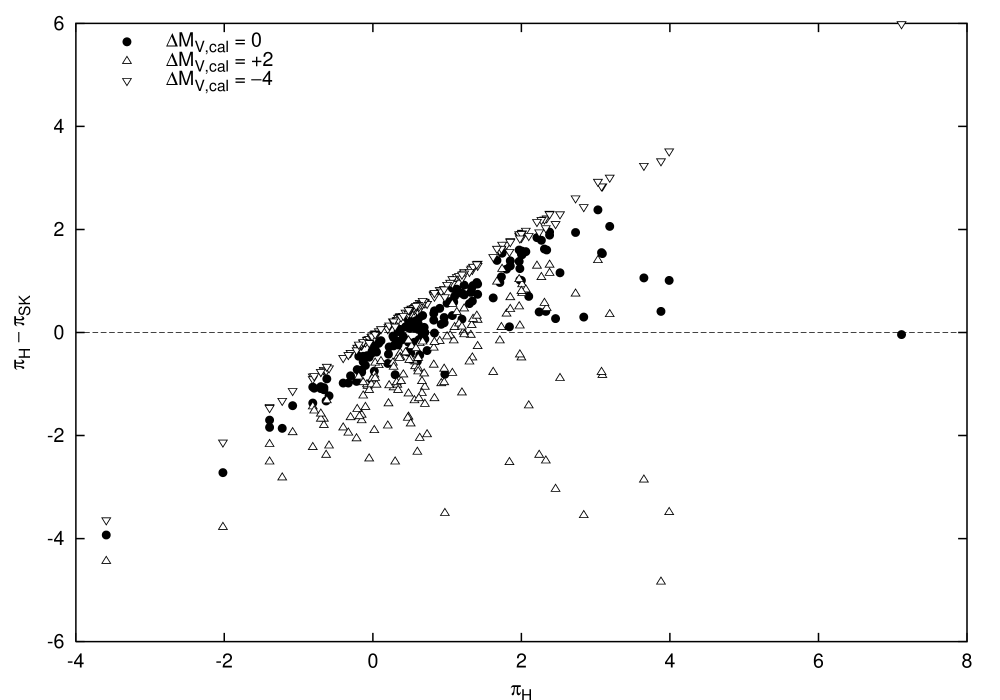
Although generally one should not straightforwardly derive the distance to individual O stars from the Hipparcos parallax measurements, it is possible to extract useful information from the full body of parallaxes. By not subjecting the observed parallax to any selection criterion we naturally avoid selection bias. Because now we also include negative ($\pi_{\rm H}<0$) and ‘unreliable’ ($\sigma_{\pi_{\rm H}}/\pi_{\rm H}>1$) parallaxes, we must revert to ‘parallax space’, which means that we do not calculate a distance or absolute magnitude, thus avoiding transformation bias. Instead, we calculate for each star the difference between the observed and expected parallax. Considering, for example, the Schmidt-Kaler et al. (1982) absolute magnitude calibration this difference is $\Delta\pi=\pi_{\rm H}-\pi_{\rm SK}$ with the expected parallax (in mas)

$$\pi_{\rm SK}=10^{3-(M_{V}^{\rm SK}-V+A_{V}-5)/5}.$$ (6)

If the calibration is correct, then on average $\Delta\pi$ should not be different from zero. Figure 4 shows the parallax difference calculated for the full body of O stars. Note that $\Delta\pi$ is limited by the line $\pi_{\rm H}-\pi_{\rm SK}=\pi_{\rm H}-0.20$, as 0.20 mas is the lowest expected parallax in our sample. We find that the average parallax difference of the stars in our sample is $\Delta\pi=0.14\pm 0.96$ mas. The Student $T$-test reveals that, indeed, this difference is not significantly different from zero at the $\alpha=0.05$ level ($T=1.76$, critical value = 1.97, df = 153). This means that the Hipparcos data are consistent with the absolute visual magnitude calibration of O stars by Schmidt-Kaler et al. (note that this test ignores individual parallax errors). When we change the absolute magnitude calibration of all spectral types by a similar amount, the average parallax difference moves away from zero, as illustrated in Fig. 4. We can change the calibration by any positive amount in the range $(0.0,0.7)$, without the average $\Delta\pi$ becoming significantly different from zero. We can apply the same test to other absolute magnitude calibrations. The Howarth & Prinja (1989) and Vacca et al. (1996) calibrations are slightly more luminous than the Schmidt-Kaler et al. calibration (the resulting average absolute magnitude of the full O star sample is $-5.4$ and $-5.5$, respectively, versus $-5.7$ for Schmidt-Kaler et al.). The Howarth & Prinja calibration is consistent with the Hipparcos data in the interval $(-0.3,0.4)$ (df = 150), whereas the Vacca et al. calibration is consistent in the interval $(-0.1,0.6)$ (df = 151).

It is important to realise what is actually being tested. Taking a closer look at Fig. 4 reveals that adjusting the absolute magnitude calibration affects the parallax difference most significantly for stars with $\pi_{\rm H}\gtrsim 2$. Consequently, the power to discriminate between different calibrations (or different calibration offsets) is largely determined by stars that are relatively nearby. Unfortunately, these do not have a homogeneous spectral distribution. Of the stars with $\pi_{\rm H}>2$, 15 have spectral type O9-9.7, 5 have type O8-8.5 and 6 have a type earlier than O8. This means that our test is predominantly one of the calibration of late spectral types. This is demonstrated by the fact that if we test only stars of late spectral type (O8-O9.7) the resulting confidence intervals are almost identical (SK: $(0.0,0.8)$, HP: $(-0.3,0.4)$, V: $(0.0,0.7)$; df = 95). If, on the other hand, we test only stars of early spectral type (O4-O7.5), we find that all calibrations are also consistent with the Hipparcos data, but with much wider confidence intervals (SK: $(-0.9,1.0)$, df = 57; HP: $(-1.3,0.7)$, df = 54; V: $(-1.2,0.7)$, df = 55).

8 Discussion

Simply deriving a distance $d_{\rm H}$ from the Hipparcos parallax $\pi_{\rm H}$ by calculating $d_{\rm H}=1/\pi_{\rm H}$ yields unreliable results for all O stars except $\zeta$ Oph and $\gamma^{2}$ Vel. That this is not general knowledge is illustrated by two examples from the literature. In our first example Van der Hucht et al. (1997) derive fundamental parameters of the spectroscopic binary $\gamma^{2}$ Vel and the O4 supergiant $\zeta$ Pup (HD 66811) using the Hipparcos parallax. While we consider the parallax of $\gamma^{2}$ Vel sufficiently accurate, deriving the distance to $\zeta$ Pup from the Hipparcos parallax seems risky, in light of our findings. Our second example involves a recent paper, in which Repolust et al. (2004) use Hipparcos parallaxes to estimate the radii of four O stars. The authors apply the Lutz-Kelker bias correction provided by Koen (1992) to $\zeta$ Oph, one of the two O stars for which the Hipparcos parallax is in fact reliable. In addition, they apply a Lutz-Kelker type correction to $\zeta$ Pup and $\lambda$ Cep (HD 210839). Not surprisingly, in light of our results, the ‘corrected’ absolute magnitude of $\lambda$ Cep does not compare well to the value expected for its spectral type. As mentioned in the previous section, in principle a parallax correction can be devised when one carefully considers properties of the stellar sample, like selection criteria and spatial distribution. But such a correction is meaningful when applied to a sample of stars, not so much to individual cases.

Table 2: Characteristics of the B stars in the sample of Lamers et al. (1997) depicted in Fig. 5. The ‘observed’ absolute magnitude $M_{V}^{\rm H}$ is calculated from the Hipparcos parallax $\pi_{\rm H}$ (in mas), and is corrected for interstellar extinction and the presence of spectroscopic companions. The predicted absolute magnitude $M_{V}^{\rm SK}$ is derived from the spectral type according to the calibration of Schmidt-Kaler et al. (1982), if necessary through interpolation (note that they have a special section for Be stars). $v\sin i$ is in km s^-1.

HD	Sp. type	$\pi_{\rm H}\pm\sigma_{\pi_{\rm H}}$	$M_{V}^{\rm H}$	$M_{V}^{\rm SK}$	$v\sin i$		HD	Sp. type	$\pi_{\rm H}\pm\sigma_{\pi_{\rm H}}$	$M_{V}^{\rm H}$	$M_{V}^{\rm SK}$	$v\sin i$
22951	B0.5V1)	$3.53\pm 0.88$	$-3.0$	$-3.6$	301)		37490	B2IIIe2)	$2.01\pm 0.94$	$-4.4$	$-4.0$	1602)
34503	B5III2)	$5.88\pm 0.77$	$-2.7$	$-2.2$	252)		143275	B0.2IV4)	$8.12\pm 0.88$	$-3.3$	$-4.5$	1484)
35468	B2III2)	$13.42\pm 0.98$	$-2.8$	$-3.9$	502)		144217	B0.5IV-V5)	$6.15\pm 1.12$	$-3.9$	$-3.9$	905)
36822	B0III3)	$3.31\pm 0.77$	$-3.1$	$-5.1$	503)		149438	B0V4)	$7.59\pm 0.78$	$-3.1$	$-4.0$	104)
References – 1) Andrievsky et al. (1999), 2) Hauck & Slettebak (1989), 3) Levato (1975), 4) Brown & Verschueren (1997), 5) Holmgren et al. (1997).

We cannot confirm the positive correlation between the stellar rotational velocity and the difference between the expected and observed magnitude found by Lamers et al. (1997), whose sample of stars is partly included in ours. To understand why they do find a correlation, we must take a closer look at their method. While ours is a large sample of exclusively O stars, they select a small number of both O and B stars for high visual brightness ($V<5.0$), a procedure that they argue should yield accurate Hipparcos parallaxes. But limiting the apparent magnitude to select for bright stars does not ensure that all are nearby, as some may be atypically bright stars located at large distances (i.e. the Malmquist bias). Moreover, the accuracy of the Hipparcos parallax can better be expressed by $\lambda=\sigma_{\pi_{\rm H}}/\pi_{\rm H}$, which is not particularly low for most of the stars in their sample. Selecting for bright stars does limit the expected magnitude difference to smaller values, as only the most distant and faintest stars can have a difference up to five magnitudes. This may explain why the magnitude difference of the stars in their sample ranges only from $-1$ to $+2$. Now, if it were not for a small group of B stars with low rotational velocity and a small positive magnitude difference, there would be no (weak) correlation (see Fig. 2 in Lamers et al.). Interestingly, the parallax of these stars has been measured with good accuracy by Hipparcos (Table 2), yet Fig. 5 shows they do not compare well with the simulated population. To ascertain that these differences are not associated with the specific spatial distribution assumed for the simulated stars (thin disk) we performed several simulations with different distributions (thick disk, spherical) and observed that the results were highly similar to those in Fig. 5. The deviation is most pronounced for HD 35468 ($\gamma$ Ori) at $\lambda=0.07$, a standard star for the B2III spectral type (Walborn 1971). It is very likely that its expected magnitude is incorrect, and possibly its spectral type. In any case, its status as a standard star needs careful re-evaluation. Three other stars are suspect (HD 34503, HD 143275, HD 149438 at $\lambda=0.13$, 0.11, 0.10, respectively), but one of these appears to be brighter instead of fainter, and another has a ‘normal’ $v\sin i$. The latter (HD 143275) is a peculiar object; this spectroscopic binary exhibits episodic Be activity (Miroshnichenko et al. 2001), which makes its expected absolute magnitude rather uncertain. Essentially, the argument that slow stellar rotation systematically hinders spectral classification of early type stars hinges on the results for one star: $\gamma$ Ori, which apparently low rotational velocity may be due to projection. In support of their original suggestion, Lamers et al. discuss that the same effect for slowly rotating B stars was already noticed by Walborn (1972) and others. Unfortunately, we cannot draw any definite conclusions for B stars due to the low number statistics. But for O stars we have shown in this paper that, at present, it is impossible to detect any correlation between the expected and observed magnitude and the rotational velocity. As of yet it is not necessary to question the validity of the luminosity class assignment to O stars as Lamers et al. suggest. Investigating whether stellar rotation needs to be taken into account in spectroscopic distance determinations will have to await future astrometric missions like GAIA, which is expected to achieve a median parallax error of 4 $\mu$as at $V=10$ (Perryman 2002).

The scope of this paper is somewhat similar to that of Wegner (2000), who devises a new absolute magnitude calibration of OB stars based on the Hipparcos results. The author eliminates negative parallaxes by applying a transformation proposed by Smith & Eichhorn (1996). As Brown et al. (1997) note, the problem with this transformation is that it lacks any physical basis, having been devised with the sole purpose of turning negative parallaxes into positive ones and render infinite variances of the computed distance finite. It has nothing to do with Lutz-Kelker type selection bias, and contrary to Wegner’s claim, by its application one does not avoid Lutz-Kelker type corrections. In fact, it may even introduce bias, judging Hanson’s (2003) observation concerning Wegner’s work that Hipparcos distances have a strong “near” bias not fully appreciated. In our view, this, together with the fact that – like ours – the sample of Wegner is heavily biased to late spectral types, severely limits the relevance of his new O star calibration, especially now that we have demonstrated that the old ones still suffice.

Figure 5: Some B stars in the sample of Lamers et al. (1997) do not compare well to the simulation at small values of $\lambda$ (compare Fig. 3), indicating that their predicted absolute magnitude may be incorrect.