VLA H92$\alpha$ and H53$\alpha$ Radio Recombination Line Observations of M82

Abstract

We present high angular resolution ($0\hbox to0.0pt{.\hss}{{}^{\prime\prime}}6$) observations made with the Very Large Array (VLA) of the radio continuum at 8.3 and 43 GHz as well as H92$\alpha$ and H53$\alpha$ radio recombination lines (RRLs) from the nearby ($\sim$3 Mpc) starburst galaxy M82. In the continuum we identify 58 sources at 8.3 GHz from which 19 have no counterparts in catalogs published at other frequencies. At 43 GHz we identify 18 sources, unresolved at $0\hbox to0.0pt{.\hss}{{}^{\prime\prime}}6$ resolution, from which 5 were unknown previously. The spatial distribution of the H92$\alpha$ line is inhomogeneous; we identify 27 features, about half of them are associated with continuum emission sources. Their sizes are typically in the range 2 to 10 pc. Although observed with poorer signal to noise ratio, the H53$\alpha$ line is detected. The line and continuum emission are modeled using a collection of HII regions at different distances from the nucleus. The observations can be interpreted assuming a single-density component but equally well with two components, if constraints originating from previous high-resolution continuum observations are used. The high-density component has a density of $\sim 4\times 10^{4}$ cm^-3. However, the bulk of the ionization is in regions with densities which are typically a factor 10 lower.

The gas kinematics, using the H92$\alpha$ line, confirms the presence of steep velocity gradient (26 km s^-1 arcsec^-1) in the nuclear region as previously reported, in particular from observations of the [Ne II] line at $12$ $\micron$. This gradient has about the same amplitude on both sides of the nucleus. As this steep gradient is observed not only on the major axis but also at large distances along a band of PA of $\sim 150^{\circ}$, the interpretation in terms of x2 orbits elongated along the minor axis of the bar, which would be observed at an angle close to the inclination of the main disk, seems inadequate. The observed kinematics cannot be modeled using a simple model that consists of a set of circular orbits observed at different tilt angles. Ad-hoc radial motions must be introduced to reproduce the pattern of the velocity field. Different families of orbits are indicated as we detect a signature in the kinematics at the transition between the two plateaus observed in the NIR light distribution. These H92$\alpha$ data also reveal the base of the outflow where the injection towards the halo on the Northern side occurs. The outflow has a major effect on the observed kinematics, present even in the disk at distances close to the nucleus. The kinematical pattern suggests a connection between the gas flowing in the plane of M82 towards the center; this behavior most likely originates due to the presence of a bar and the outflow out of the plane.

1 INTRODUCTION

M82 is an excellent candidate to investigate the physical conditions of a starburst galaxy because it is one of the nearest ($\sim$3 Mpc) and brightest objects of this class. The bulk of the ionized gas in this galaxy is located in regions that are surrounded by large amounts of dust: in M82 the extinction in visual magnitudes, A_V, ranges from a few to about 15 mag. Radio-wavelength observations, which are not affected by dust obscuration, can play a key role in the determination of the physical properties of the ionized gas in starburst galaxies.

M82 has been observed in the radio continuum over a wide range of frequencies (Kronberg, Biermann & Schwab 1985; McDonald et al. 2002) and is known to host a population of compact sources as observed at angular resolutions $<0\hbox to0.0pt{.\hss}{{}^{\prime\prime}}$2 (McDonald et al. 2002 and references therein). The total number of compact sources decreases at 20 cm as compared to 2 cm; this result has been interpreted as due to free-free absorption by ionized gas in compact HII regions. Of the 46 compact sources identified by McDonald et al. (2002), $\sim 35\%$ were classified as HII regions based on their continuum spectra.

The distribution and kinematics of the ionized gas in the central kiloparsec of M82 have been previously studied using radio recombination lines (RRLs). The first detections of RRLs from M82 (Seaquist & Bell, 1977; Chaisson & Rodríguez, 1977) were a major achievement that led to further investigations of extragalactic RRLs. VLA observations of RRLs up to 8 GHz by Anantharamaiah & Goss (1990) toward NGC 253 motivated further interferometric observations of RRLs at the same frequency (Anantharamaiah et al., 1993; Zhao et al., 1996; Mohan et al., 2002) and higher frequencies (Zhao et al., 2000; Anantharamaiah et al., 2000) toward starburst galaxies. Using the total integrated line emission, global estimates were made for the properties of the ionized gas in M82 (Seaquist, Bell & Bignell, 1985). Using the Westerbork Synthesis Radio Telescope, Roelfsema (1987) obtained the velocity field at moderate angular resolution ($\sim 13^{\prime\prime}$) using the H166$\alpha$ RRL (at 1.4 GHz). These observations show the rotation of the ionized gas in the central 600 pc, with solid body rotation within a radius of $\sim 170$ pc or $8^{\prime\prime}$. The velocity field has also been obtained using the [Ne II] line in the mid IR with $2^{\prime\prime}$ angular resolution (Achtermann and Lacy, 1995). The velocity fields obtained from the H166$\alpha$ and the [Ne II] line observations are not consistent, specially in the SW half. However, the different angular resolutions achieved for each line prevent a direct comparison. Higher angular resolution observations of RRLs were necessary to understand the kinematics of the ionized gas. Seaquist et al. (1996) observed the H41$\alpha$ line with angular resolution of 4^′′ and, in addition to the normal rotation, they showed the presence of kinematical features with velocity deviations up to 150 km s^-1. From observations of the ¹²CO, ¹³CO and ¹⁸CO lines, Weiss et al. (1999) and Matsushita et al. (2000) reported evidence for an expanding supershell on the SW side of the nucleus of M82.

The high level of star formation activity at the center of M82 could have been triggered due to the close interaction with the neighboring galaxy M81 and the presence of a bar that would drive the gas inwards to feed the starburst. From observations of the morphology and the kinematics of the different constituents in the inner part of M82, the presence of x1 and x2 orbits has been suggested to indicate the existence of a bar (Achtermann and Lacy, 1995; Wills et al., 2000; Greve et al., 2002). In this scenario, the ionized gas is mainly found along the x2 orbits i.e. highly confined near the center. X-ray observations also suggests the presence of a low luminosity AGN in M82 (Matsumoto & Tsuru, 1999).

The interpretation of the RRLs is not straightforward since the line emission mechanism could involve three different contributions: spontaneous as well as internal and external stimulated emission. The radio continuum emission in the starburst regions has contributions from free-free (thermal) and synchrotron (non-thermal) radiation, which also leads to complexity in the interpretation of the observations. Using the radio continuum and RRL observations, Anantharamaiah et al. (2000) developed a model that consists of a collection of HII regions in order to determine the physical properties of the ionized gas in Arp 220. These authors have been able to reproduce the observations in the frequency range $0.15-113$ GHz and the simultaneous existence of both low density ($\sim$10³ cm^-3) extended ($\sim$5 pc) HII regions and high-density ($\sim$10⁵ cm^-3) ultra-compact ($\sim$0.1 pc) HII regions was deduced.

In this paper, using the Vey Large Array (VLA) of the National Radio Astronomy Observatory (NRAO), we present observations toward M82 of the radio continuum at 8.3 and 43 GHz and the H92$\alpha$ (3.6 cm) and H53$\alpha$ (7 mm) RRLs. With an angular resolution of $0\hbox to0.0pt{.\hss}{{}^{\prime\prime}}6$ ($\sim$9 pc), we can obtain detailed information of the spatial distribution and kinematics of the ionized gas within the central starburst region. In particular we search for continuum emission sources associated with the H92$\alpha$ and H53$\alpha$ line emitting regions. This paper is organized as follows: the observations are discussed in $\S$ 2; the results are presented in $\S$ 3; a model, based on the observations of radio continuum and RRLs, that consists of a conglomerate of HII regions is presented in $\S$ 4; a discussion of the radio continuum emission at 8.3 and 43 GHz, the implications of the kinematics and the results of the proposed model are discussed in $\S$ 5; and finally, the conclusions are summarized in $\S$ 6.

2 OBSERVATIONS.

2.1 8.3 GHz data.

2.1.1 Observations and calibration

The observations of the H92$\alpha$ line ($\nu_{rest}=$8309.3832 MHz) were conducted in the C (April 22, 1996), CnB (Feb 13, 2000) and B (May 05 and 11, 2001) VLA configurations. The maximum angular resolution achieved is $\sim 0\hbox to0.0pt{.\hss}{{}^{\prime\prime}}6$. The observations made in the C array have been acquired from the VLA archive database. The 31 spectral channels mode was used with a total bandwidth of 25 MHz, corresponding to a velocity coverage of $\sim$850 km s^-1, centered at a heliocentric velocity of 200 km s^-1. The flux density scale was determined by observing 3C286 (5.3 Jy at 3.6 cm). The phase calibrator was 1044+719, with a flux density of 1.5 Jy. The bandpass calibration was made using the calibrator 3C48 with a flux density of 3.2 Jy. Bandpass calibration is critical in these observations because the line-to-continuum ratios are $\leq 1$%. The data were Hanning-smoothed offline to improve the signal-to-noise ratio (S/N) and minimize the Gibbs effect. The effective velocity resolution is 56 km s^-1 (806 kHz). Each of the databases were self-calibrated in phase using the continuum channel; the solutions were then applied to the spectral line data. The data sets taken at different epochs were combined into a single data set. The self-calibration process was further used on this data set to correct for small phase offsets between the individual observations. The AIPS task UVLSF was used to estimate the continuum level by fitting a linear function through the spectral channels free of line emission, and then subtracted from each visibility record. The observational parameters for the H92$\alpha$ line are listed in Table 1.

2.1.2 Imaging.

The use of a natural weighting scheme for the data in the C configuration relative to those in the B configuration produces a synthesized beam with prominent wings (at the level of 2%). In order to correct this problem, we use a technique that consists of re-weighting the data in the u,v plane so as to produce a gaussian beam in the image. After the re-weighting process, if necessary, the image is deconvolved using the CLEAN algorithm. Because the u,v plane is properly sampled in the inner region, the deconvolution is not required when producing images at an angular resolution of $2^{\prime\prime}$ FWHM. For the images made at angular resolutions of $0\hbox to0.0pt{.\hss}{{}^{\prime\prime}}6$ and $0\hbox to0.0pt{.\hss}{{}^{\prime\prime}}9$ (section 3), a deconvolution is required. In these cases the $2^{\prime\prime}$ angular resolution image is used as an input for regularization in the process of deconvolution. The quality of the final images is limited by errors due to the imperfect continuum subtraction. These errors appear as weak fluctuations over a scale of one arcmin. These fluctuations have a typical correlation length of about 4 MHz along the spectral axis. This behavior results in systematic errors which limit the quality of the “baselines” ($\sim 2\%$) in the spectra produced from different regions of M82 for our data analysis.

2.2 43 GHz data

2.2.1 Observations and calibration

The observations of the H53$\alpha$ line ($\nu_{rest}=$42951.9714 MHz) were carried out in the C array of the VLA on April 13, 2000. The VLA correlator is limited to a bandwidth of 50 MHz ($\sim$350 km s^-1 at 7 mm). At 43 GHz three adjacent spectral windows, each of them with 15 channels, are required to cover the velocity range of the RRL ($\sim$600 km s^-1). The windows were centered at 42185.1, 42214.9 and 42235.1 MHz. The amplitude, phase and bandpass calibrators used were 3C286 (1.47 Jy), 0954+658 (0.87 Jy) and 1226+023 (19.4 Jy), respectively. The flux density calibrator was observed only for the central LO window (42214.9 MHz). The flux densities of the phase and bandpass calibrators in the adjacent LO windows (42185.1 and 42235.1 MHz) were assumed to have the same values as those determined from the central LO window. The phase calibrator was observed at time intervals of 10 min. The on-source integration time was $\sim$2 hrs for each frequency window. The bandpass response of the instrument is different for each frequency window; the observation of both the bandpass and the phase calibrator must be interleaved between the different overlapping frequency windows required to observe the complete line. This method removes the offsets ($\leq 5\%$) between the frequency windows. In order to correct for phase decorrelation that may be present for time intervals $<$8 min, a phase calibration was performed initially followed by a second calibration step applied to both phase and amplitude. Phase correction is more important at these frequencies since the troposphere introduces phase offsets that may affect the coherence of the data. The line-to-continuum ratio for this line is $10-20\%$ in the brightest region of M82. Table 1 shows the details of the observations for the H53$\alpha$ line.

2.2.2 Imaging.

In order to produce the H53$\alpha$ line image, the contribution of the continuum emission must be removed and the three frequency windows combined. The method uses two a priori constraints on the source model that are not independent. The first constraint is set by assuming that the emission in the lowest spatial frequencies is mostly continuum emission, allowing us to clip the data for the shortest spacings in the u,v plane. The second constraint is based on the fact that the projected velocity of the gas in M82 varies across the image due to the rotation of the galaxy. Hence, if we include a priori information on the rotational properties of M82, for each position in the image, we can maximize the number of line-free channels in each LO setting to reduce the uncertainties when removing this contribution. As a result this second method involves the following steps for each LO setting: (1) filter out part of the emission present at the lowest spatial frequencies, (2) produce an undeconvolved 3-dimensional image, (3) determine the level of remaining continuum for each position, (4) determine the offsets by comparing these levels from one LO setting to the other for each position, (5) refine the determination of this remaining continuum by including the line-free channels of the adjacent LO settings for each position, (6) subtract the determined continuum contribution and (7) average the three spectral windows to make the single 3-dimensional line image. It is not necessary to deconvolve the results after step 6 because the signal-to-noise ratio for the line emission is between 2 and 5.

In order to produce the 43 GHz continuum image we carried out the following steps: (1) produce a raw 3-dimensional image for each LO setting, (2) subtract the line contribution as derived above in each LO setting, (3) determine the mean continuum level for each position in each LO setting, (4) average the three 2-dimensional images obtained in step 3 and also average the three synthesized beams and (5) finally deconvolve this averaged image.

The undeconvolved images were generated using the AIPS IMAGR program applying the suitable u,v tapers to obtain images at different angular resolutions. They were further processed in the GIPSY environment to perform all the subsequent steps. The data were Hanning-smoothed offline and a final spectral resolution of 44 km s^-1 was achieved.

3 RESULTS

Globally, from the 8.3 GHz data, we obtain a total integrated continuum flux density of 2.6$\pm$0.1 Jy and a H92$\alpha$ line flux density of 2.9$\pm$0.1 Jy km s^-1. At 43 GHz the total continuum flux density is in this case 0.82$\pm$0.16 Jy and the H53$\alpha$ line flux density is 3.0$\pm$0.2 Jy km s^-1. Images at three different resolutions are produced to analyze the data. The high angular resolution ($0\hbox to0.0pt{.\hss}{{}^{\prime\prime}}6$) images are suitable to investigate the compact bright features. Using the intermediate resolution images ($0\hbox to0.0pt{.\hss}{{}^{\prime\prime}}9$), it is possible to study the weak extended features with sufficient angular resolution. The low angular resolution images ($2^{\prime\prime}$) provide information on the overall distribution of the ionized gas.

3.1 Radio continuum at 8.3 and 43 GHz

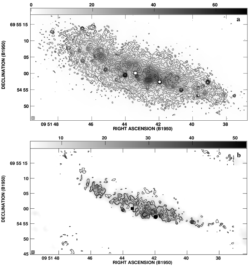
A correction for the primary beam was applied to the images at 8.3 GHz and 43 GHz. In the images at 8.3 GHz this correction does not exceed $\sim$2%, while for the 43 GHz images this correction is a factor of 1.2 at the extreme edges of M82. The radio continuum images at 8.3 and 43 GHz are shown in Fig. 1a and Fig. 1b, respectively; the high angular resolution images (contours) are shown overlaid on their corresponding low angular resolution images (gray scale) at each frequency.

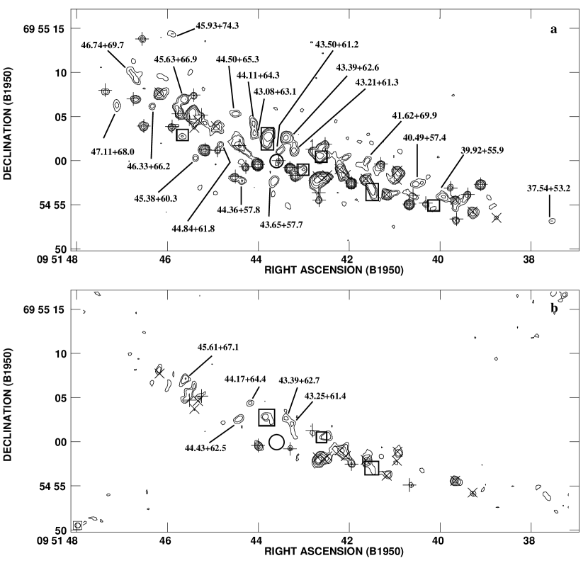
A number of previous high angular resolution ($\leq 0.1^{\prime\prime}$) studies carried out over the range 408 MHz to 15 GHz have revealed the existence of a population of compact sources classified as HII regions or SNRs (Kronberg et al., 1985; Huang et al., 1994; Muxlow et al., 1994; Wills et al., 1997; Allen & Kronberg, 1998; McDonald et al., 2002). In order to study the small scale continuum features at 8.3 GHz, the underlying extended emission was filtered out by restricting the lower uv-baseline range (to u,v distances larger than 50 k$\lambda$) so that no structures larger than 4^′′ are present. At 43 GHz an iterative procedure is used to determine and remove the spatially extended continuum emission. Figures 2a and 2b show the resulting spatial distribution of these features at 8.3 and 43 GHz, respectively. In these images we are able to identify $\sim 85\%$ of the previously known compact sources. The remaining $15\%$ of compact sources were not detected because their peak flux density is below the level of the local diffuse emission. On the other hand, these images reveal 21 new features (19 of these sources are detected at both frequencies and two sources only at 43 GHz) not detected in previous studies. Several of these sources are relatively more extended ($>0\hbox to0.0pt{.\hss}{{}^{\prime\prime}}5$) and they could not be identified in the previous high angular resolution images. Including our new detections, a total of 60 sources are detected toward M82, 58 features at 8.3 GHz and 18 at 43 GHz.

In Table 2 we list the parameters of these 60 compact features:

• The first column lists the galactic names for each source. For each feature we measure its spatial position, its deconvolved angular size and flux density. The measurements at 8.3 GHz are summarized in columns 2, 3 and 4 and those at 43 GHz in columns 5, 6 and 7, respectively. For the 21 newly detected features a super-script “a” is used. The uncertainties in flux densities correspond to a 1 $\sigma_{rms}$ noise in the least-squares fitting procedure. For features not detected, we provide an upper limit of 3 $\sigma_{rms}$ for the flux densities.

• From the measured flux densities (columns 4 and 7) we derive the spectral index (column 8) between 8.3 and 43 GHz. This value can be compared with the spectral index previously reported in the literature (column 9) using different frequency ranges (e.g. 0.408 to 15 GHz).

• In column 10 we list identifications for the sources which have radio recombination line emission. The associations are made with the H92$\alpha$ line features observed at 0$\hbox to0.0pt{.\hss}{{}^{\prime\prime}}$9 (see section 3.2). At an angular resolution of 0$\hbox to0.0pt{.\hss}{{}^{\prime\prime}}$6, only four H92$\alpha$ compact line features are detected with signal-to-noise ratio $>3$ (see section 3.2 and Fig 3).

• In the last column, the classification is given (HII regions or SNR). The sources previously identified as HII regions by McDonald et al. (2002) were classified based on their spectral indexes, $\alpha$, which in these cases are inverted ($S_{\nu}\propto\nu^{\alpha}$, $\alpha>0$) between 5 and 15 GHz (column 9). We confirm the classification for all the HII regions previously reported, as they have a spectral index that is consistent with optically thin free-free emission between 8.3 and 43 GHz (column 8). We assign tentatively an HII type to four more features, because between 8.3 and 43 GHz, 43.21+61.3 and 45.63+66.9 have flat spectra and 44.17+64.4 and 44.43+62.5 have inverted spectra. For the sources previously identified as SNRs, our results show non-thermal spectra between 8.3 and 43 GHz (see column 8) as expected from the spectral index computed between 5 and 15 GHz. In addition to those features previously classified as SNRs, based on the upper limits obtained from the spectral index between 8.3 and 43 GHz, we can tentatively consider 39.92+55.9, 40.49+57.4, 43.00+59.0, 44.11+64.3 and 46.74+69.7 as SNRs. It is noted that three SNRs, 41.29+59.7, 43.00+59.0 and 45.79+65.2, exhibit H92$\alpha$ RRL emission; this issue will be discussed in $\S$ 5.

3.2 Radio Recombination Lines H92$\alpha$ and H53$\alpha$

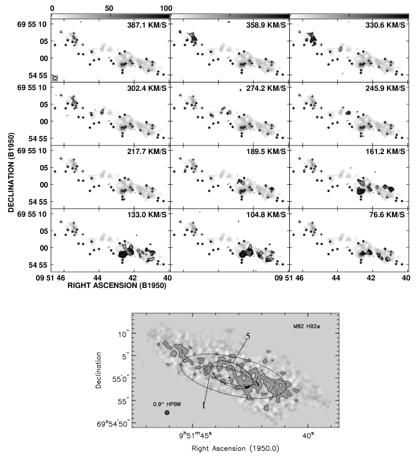
Figure 3 shows the high-resolution ($0\hbox to0.0pt{.\hss}{{}^{\prime\prime}}6$) H92$\alpha$ line images in the region where H92$\alpha$ RRL emission is detected; in these images four sources are clearly identified. The center of this region is located $\sim$4^′′ W of the 2.2 $\mu$m peak (Lester et al., 1990) and corresponds to the brightest area observed in the H92$\alpha$ line in M82 on a larger scale. All four line emitting sources are spatially associated with compact continuum sources previously identified by McDonald et al. (2002). No other line features are detected outside this region at this resolution. For Figure 4 we show the velocity-channels at an intermediate angular resolution of $0\hbox to0.0pt{.\hss}{{}^{\prime\prime}}9$ (top) and an image of the total integrated H92$\alpha$ line emission (bottom). In this case 27 line features can be identified and those associated with continuum sources are listed in column (10) of Table 2. In these images, the position of the HII regions (crosses) and SNRs (stars) are shown as reported by McDonald et al. (2002). In this comparison the SNRs are mainly located at the periphery of the line emitting regions while the HII regions are clearly associated with the RRL emission. Because these HII regions are the compact continuum sources which have inverted spectra between 5 and 15 GHz (section 3), we have direct evidence that this population of compact objects is associated with the more extended HII regions which produce the H92$\alpha$ recombination line emission. Figure 5 (top) shows the H92$\alpha$ line velocity-channels at a low angular resolution of $2^{\prime\prime}$ (top) for the overall distribution of the integrated H92$\alpha$ line emitting regions (bottom).

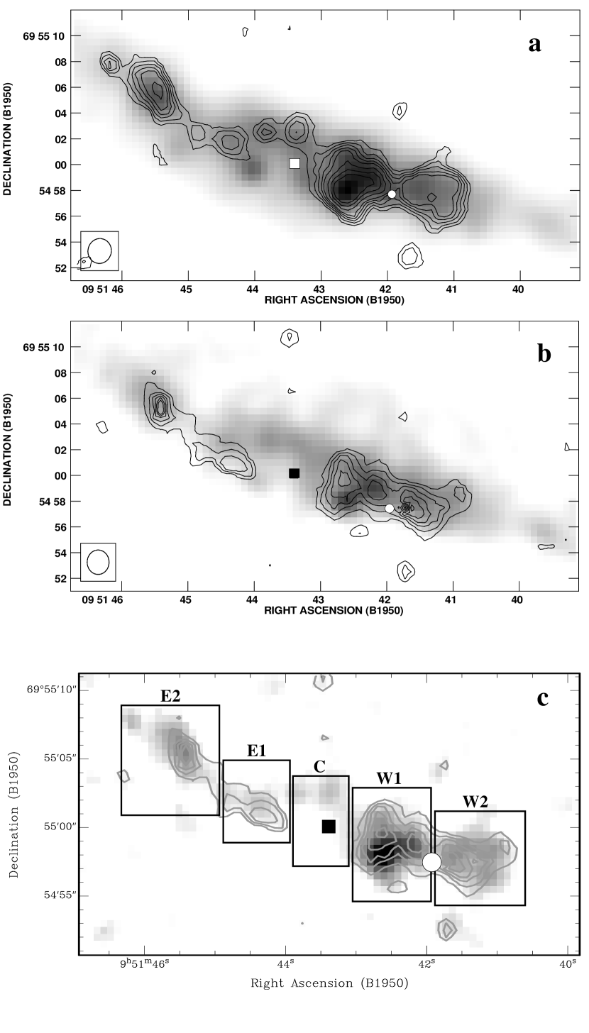
Figures 6a and 6b show the low-resolution images of the integrated H92$\alpha$ and H53$\alpha$ line emission (contours) overlaid on the low-resolution images of radio continuum at 8.3 and 43 GHz (gray scale), respectively. To produce these images for the integrated line emission only the regions with line emission $>3\sigma_{rms}$ were selected. There is a clear correspondence between the spatial distribution of the line and the continuum emissions. In both cases the distribution of the total line emission is characterized by a pair of concentrations on each side of the center defined by the 2.2 $\mu$m peak (Lester et al., 1990). However, the sources located on the E side are fainter compared with their counterpart on the W side. This asymmetry has also been observed in [Ne II] and for several molecules (Achtermann and Lacy, 1995). Figure 6c shows the velocity integrated line emission of the H53$\alpha$ line (contours) overlaid on the corresponding image of the H92$\alpha$ line (gray scale). A good correspondence between the spatial distributions for the two lines is observed. Both lines cover an angular size of about $30^{\prime\prime}$ (480 pc) along the major axis and the main peak is $\sim 4^{\prime\prime}$ W of the 2.2 $\mu$m peak. However, we note that the H92$\alpha$ line emission may be more extended than the H53$\alpha$ line emission ($\sim$ 4^′′) on the extreme NE side of M82. More sensitive H53$\alpha$ line observations would be required to verify this possible difference. In order to characterize the physical properties of the ionized gas in M82 (section 4.2), we define five regions ( E1, E2, C, W1 and W2) as indicated by the rectangular boxes in Figure 6c. Regions E1, W1 and W2 have been labeled according to peaks observed in [Ne II] emission (Achtermann and Lacy, 1995). The comparison of the distribution of the H92$\alpha$ line emission with the distribution of other tracers of the ionized gas is discussed in $\S$ 5.2.

Figure 7 shows the spatially integrated H92$\alpha$ and H53$\alpha$ spectra for four distinct regions ( E1, E2, W1 and W2); the spectrum for region “C” is not shown since H53$\alpha$ line emission is not detected above 3$\sigma_{rms}$. The area for the integration of line and continuum emission are defined by the first contour (57 Jy beam^-1 m s^-1) of the H53$\alpha$ distribution. The H92$\alpha$ and H53$\alpha$ line parameters derived from the fits of gaussian profiles (Figure 7) are given in Table 3. Columns (2), (3) and (4) of Table 3 list the parameters obtained for the RRL H92$\alpha$ and column (5) the continuum flux density at 8.3 GHz. Columns (6), (7) and (8) list the parameters obtained for the RRL H53$\alpha$, column (9) the continuum flux density at 43 GHz, column (10) the maximum filling factor for the high-density component explained in $\S$ 4 and column (11) the continuum flux density at 5 GHz (personal communication, A. Pedlar). These measurements form the basis for the models discussed in $\S$ 4.

The global properties for the five regions identified in Figure 6c are given in Table 4, the total H92$\alpha$ line emission integrated over each rectangular box (column 2) and the corresponding line (H92$\alpha$) to continuum (at 8.3 GHz) ratio (column 3). Inside these four regions a number of sub-regions have been identified in the H92$\alpha$ line image (see Table 4). For each of these sub-regions (labeled in column 4), Table 4 lists the spatial coordinates (column 5), the velocity-integrated line emission (column 6), the FWHM angular size deconvolved to correct for the $0\hbox to0.0pt{.\hss}{{}^{\prime\prime}}9$ beam broadening (column 7), the peak flux density (column 8), centroid velocity (column 9) and the spectral width (column 10). The angular size of each sub-region is based on fits of 2D gaussians in the appropriate spectral channels; the spectral line parameters were obtained fitting a gaussian profile along the spectral axis for the spatially integrated emission in each of these sub-regions. For each region the sum of the line flux densities of the sub-regions is also given and can be compared with the total line flux density in column 2, determined from the low angular resolution image. For all regions, essentially all the line flux density arises from these sub-regions. Thus, any diffuse emission is $\leq 10\%$.

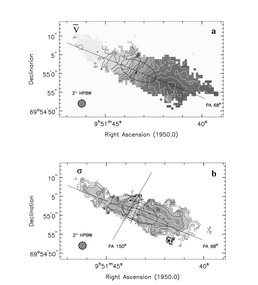
The velocity field determined using the H92$\alpha$ line image at 2^′′ angular resolution is shown in Figure 8a. In this image, the major and minor axis are indicated for a disk with a diameter of 40^′′ as observed at an inclination of $81^{\circ}$, and position angle (PA) of $68^{\circ}$ relative to the observer. The intersection of these two axes is set at the position of the 2.2 $\micron$ peak (Dietz et al., 1986), which also coincides with the center of the hole in Fig. 5b. The position of the center of the ring fitted by Achtermann and Lacy (1995), assumed to be the kinematic center, is indicated by a cross. The important features in this velocity field are the following: a) The major axis corresponds to the line of nodes which gives the maximum velocity gradient for the outer regions, b) in the central region there is a significant tilt of the iso-velocities relative to the PA of the minor axis, c) this velocity field is dominated by an axisymmetric pattern and the position of the center of symmetry appears to have a small offset ($\sim 1\hbox to0.0pt{.\hss}{{}^{\prime\prime}}5$) relative to the position of the 2.2 $\micron$ peak, d) Some areas show significant deviations relative to this general pattern, in particular in the region near 9^h51^m43$\hbox to0.0pt{.\hss}{{}^{s}}$5, +69^∘55^′04^′′, where the velocities are $\sim 40$ km s^-1 larger than expected. The kinematics of the ionized gas are discussed in $\S$ 5.3. The spatial distribution of the velocity dispersion is shown in Figure 8b. One important feature in this image is the presence of a band $\sim 1\hbox to0.0pt{.\hss}{{}^{\prime\prime}}5$ wide with a PA of $\sim 150^{\circ}$, close to the minor axis, where the spectra are systematically narrower. This feature is analyzed in section 5.3.

4 Models with multiple HII regions.

In three starburst galaxies (Arp 220, M83, NGC 2146) a model consisting of a collection of HII regions has been used successfully to explain the observations of RRLs and the radio continuum (Anantharamaiah et al., 1993; Zhao et al., 1996; Anantharamaiah & Goss, 1996; Anantharamaiah et al., 2000). The ionized gas distribution in the center of M82 is inhomogeneous as observed in the RRLs H92$\alpha$ and H53$\alpha$. Thus, a model that consists of a collection of HII regions seems appropriate to explain the RRL and radio continuum emission from this galaxy. Based on this model we can derive the physical parameters of the HII regions (e.g. electron temperature and volume density). The model must reproduce both the observations of the line and continuum emission as a function of frequency. For M82, observations at 2^′′ angular resolution of RRLs are available at two different frequencies (8.3 and 43 GHz) and observations of radio continuum at three frequencies (5, 8.3 and 43 GHz). The 5 GHz flux densities are listed in column 11 of Table 3.

The gas is ionized by young massive stars (types O and/or B) radiating large amounts ($\geq 10^{49}$ s^-1) of Lyman continuum photons. The number of Lyman continuum photons determines the size, $l$, of each HII region depending on the electron density. Since these models are constructed to obtain average values for the physical properties of the ionized gas, we have assumed: (1) Each ionizing massive star emits the same number of Lyman continuum photons (N${}_{Lyc}=10^{49}$ $s^{-1}$) and (2) N_Lyc is related to the electron density and the size of each HII region by $N_{Lyc}\propto n_{e}^{2}l^{3}$; this relation implies that for each density value, $l$ will be determined and then $l$ is not a free parameter in the model, providing a constraint. Since massive stars have a relatively short lifetime on the main sequence, the derived number of Lyman continuum photons can be related to the star formation rate (SFR) of O and B stars if the absorption of Lyman continuum photons by dust inside the HII regions is neglected.

This model consists of HII regions located in front of a diffuse mixture of thermal and non-thermal emission (S_Cbg). The HII regions radiate free-free emission and recombination lines. Background non-thermal emission and free-free emission that arise inside each HII region may stimulate the emission of RRLs in the HII regions. Thus, the line emission from each HII region has three different contributions: (i) spontaneous, (ii) internally stimulated and (iii) externally stimulated emission. Each HII region is characterized by an electron temperature $T_{e}$ (K), electron density $n_{e}$ (cm^-3), and linear size $l$ (pc). The thermal continuum flux density, S_C-TH, is given by,

$$S_{C-TH}=\Omega_{HII}B_{\nu}(1-e^{-\tau_{c}})~{}mJy,$$ (1)

where $\Omega_{HII}$ is the solid angle subtended by each HII region, $B_{\nu}$ is the black-body emission (mJy) and $\tau_{C}$ is the continuum optical depth, which depends on frequency $\nu_{L}$ as follows (Bell & Seaquist, 1978):

$$\tau_{C}=3.01\times 10^{-2}\nu^{-2}T_{e}^{-1.5}ln\bigg{(}\frac{4.95\times 10^{-2}T_{e}^{1.5}}{\nu_{L}}\bigg{)}EM_{C},$$ (2)

where $EM_{C}=n_{e}^{2}l$ is the emission measure for each HII region. The line flux density, $S_{L}$ (mJy), arising from each HII region is calculated using,

$$S_{L}=\frac{2k\nu^{2}}{c^{2}}\Omega_{HII}T_{e}\biggl{[}\frac{b_{n}\tau_{L}^{*}+\tau_{c}}{\tau_{L}+\tau_{c}}(1-e^{-\tau_{L}+\tau_{c}})-(1-e^{\tau_{c}})\biggr{]}+S_{Cbg}e^{-\tau_{c}}(e^{-\tau_{L}}-1)~{}mJy.$$ (3)

The spontaneous and the internally stimulated emission are represented by the first term in Eq. 3 and the externally stimulated emission is represented by the second term. $k$ is the Boltzmann constant, c is the speed of light, $\tau_{L}^{*}$ is the peak line optical depth under LTE conditions, $\tau_{L}=b_{n}\beta_{n}\tau_{L}^{*}$ is the peak line optical depth corrected for non-LTE effects, $b_{n}$ is the departure coefficient, $n$ is the quantum number, and $\beta_{n}=1-(kT_{e}/h\nu_{L})dlnb_{n}/dn$. For a given combination of parameters T_e and n_e, we compute the corresponding values of $b_{n}$ and $\beta_{n}$ (Salem & Brocklehurst, 1979) which are used to calculate the integrated line flux density of a single HII region using Eq. 3. The line optical depth is given by $\tau_{L}^{*}=\tau_{c}S_{L}/S_{C-TH}$ where the line to thermal continuum ratio in LTE is defined as,

$$\frac{S_{L}}{S_{C-TH}}=2.33\times 10^{4}\Big{(}\frac{\Delta\nu_{L}}{kHz}\Big{)}^{-1}\Big{(}\frac{\nu_{L}}{GHz}\Big{)}^{-2.1}\Big{(}\frac{T_{e}}{K}\Big{)}^{-1.15}\frac{EM_{L}}{EM_{C}},$$ (4)

where EM_L is the emission measure from hydrogen and EM_C is the emission measure from all ions (cm^-6 pc). In these models, EM_L/EM${}_{C}=1$; for simplicity we do not consider the presence of ionized He.

Single-density (SD) models, consisting of a number of HII regions with the same physical properties, have been used to reproduce the observations. Additionally, following Anantharamaiah et al. (2000), two-density (TD) models that consist of both low- and high-density HII regions were used to reproduce the observed values (listed in Table 4) for four regions ( E1, E2, W1, W2); in region ’C’ the H53$\alpha$ line emission is not detected (see Figure 6c). The following constraints have been imposed: (i) the predicted thermal radio continuum flux densities should not exceed the radio continuum flux density observed at 43 GHz, (ii) the area filling factor should be $\leq 1$, (iii) the peak line emission from the model should not be larger than the corresponding observations, (iv) the spectral index of the background radiation has been limited to be not steeper than $-$1.5, (v) the continuum computed from the model must reproduce all continuum observations at 6 cm, 3.6 cm and 7 mm, and (vi) the area filling factor for the high-density component has an upper limit imposed by observations of compact continuum sources at high angular resolution (McDonald et al., 2002). For the two-density models the constraint (vi) is based on the additional assumption that the high-density HII regions are coincident with compact sources previously identified as HII regions. Using the emission measure given in Table 4 of McDonald et al. (2002), we compute the angular sizes and the maximum filling factor for the HII regions that form the high-density component. The models that are consistent with these constraints were accepted as valid solutions.

The number of HII regions for the single-density model is computed by dividing the observed integrated line flux density by the integrated line flux density from a single HII region. In the case of the model with two-density components, the number of HII regions with high-density gas (N_HII-HD) is computed dividing the area filling factor derived above by the area filling factor that a single high-density HII region can occupy (following $n_{e}\propto l^{-3/2}$). Once we know the contribution of the high-density component to the line and continuum emission, the number of HII regions in the low-density component (N_HII-LD) can be estimated (see Table 5) .

For both the single-density and the two-density models, the contribution from the background emission is computed as the difference between the observed radio continuum at 8.3 GHz and the value predicted by the models for the thermal emission at this frequency. The spectral index value ($\alpha$), determined for this background emission, is obtained by minimizing the difference between the observed and the predicted values of the thermal continuum flux density at 43 GHz.

Since we have assumed that each HII region is being excited by stars that emits N${}_{Lyc}=10^{49}$ photons per second, the total rate of emission of ionizing photons, N_Lyc-tot, is,

$$N_{Lyc-tot}=N_{Lyc}N_{HII},$$ (5)

where $N_{HII}=N_{HII-LD}+N_{HII-HD}$. Another way to estimate N_Lyc-tot is using (Schraml & Mezger, 1969; Rodríguez et al., 1980),

$$\bigg{[}\frac{N_{Lyc-tot}}{s^{-1}}\bigg{]}=9.0\times 10^{43}\bigg{(}\frac{S_{C-TH}}{mJy}\bigg{)}\bigg{(}\frac{Te}{10^{4}~{}K}\bigg{)}^{0.35}\bigg{(}\frac{\nu}{4.9~{}GHz}\bigg{)}^{0.1}\bigg{(}\frac{D}{kpc}\bigg{)}^{2},$$ (6)

where we can use the flux density from thermal emission, $S_{C-TH}$, at any frequency (if $\tau_{C}<<1$) and D, the distance to the galaxy. In the case of optically thin emission at 43 GHz, both estimates of N_Lyc give similar values. However, the model is based on a number of assumptions. On the other hand, the number of Lyman continuum photons is proportional to the radio continuum at 43 GHz and does not depend on extinction estimation as occurs for the near-infrared case. Thus, the determination of the number of Lyman continuum photons from the continuum at 43 GHz is the most reliable way to estimate the Lyman continuum photons production. If the gas is optically thick (which may be the case for a high-density component) at 43 GHz, then the estimation of the total number of ionizing photons using Eq. 5 is a lower limit. The total SFR can be derived from the Lyman continuum luminosity following Anantharamaiah et al. (2000).

4.1 Results from the models.

The parameters T_e and n_e were considered to lie in the ranges $5000-10,000$ K (Garay & Rodríguez 1983) and 500-10⁶ cm^-3, respectively. The low-density component was defined to consist of HII regions with electron density, n_e in the range 100$-$10⁴ cm^-3, while the high-density component was defined as composed of HII regions with n_e in the range $2\times 10^{4}-10^{6}$ cm^-3. In Table 5 we list the range of physical parameters estimated using the models for each identified complex of HII regions (see Fig. 6c). For each identified complex of HII regions, Table 5 lists: the size of each HII region, number of HII regions, factor of area covered by each density component, number of ionizing photons, star formation rate, line and continuum opacity at 8.3 GHz, the departure coefficients for the H92$\alpha$ line, the spectral index of the background emission and the total mass of ionized gas. Figure 9 shows the expected variation of radio continuum and the integrated RRL strength as a function of frequency for regions E1, E2, W1 and W2. The models shown in Figure 9 correspond to the mean values based on the models listed in Table 5.

The single-density models reproduce the observed line and continuum flux densities for all regions considered. However, these results only provide a rough estimate for the physical properties of the ionized gas. As we know from previous studies (McDonald et al., 2002), there are compact HII regions in which higher density gas ($>10^{3}$ cm^-3) could be present. Using the area filling factor constraint in the two-density models (see section 4), we obtain valid solutions for regions E2, W1 and W2. These two densities are a few $10^{3}$ cm^-3 and $10^{4}$ cm^-3 as listed in Table 5. For the region E1, there is no evidence of any compact high-density HII regions (McDonald et al., 2002). Since for region E1 we do not have an area filling factor constraint, an estimate of the physical properties of the high-density ionized gas was not computed.

Based on these models the area filling factor from all HII regions, including the cases where the high-density component is taken into account, is $\sim 0.3$. We consider that the number of HII regions (obtained from the models) in the compact features is an upper limit. As listed in Table 5, the low-density ionized gas has an electron density of $\sim 5\times 10^{3}$ cm^-3. McDonald et al. (2002) found that the turnover in the spectrum of SNRs at 1.4 GHz requires foreground emission measures of $\sim 10^{7}$ pc cm^-6, consistent with our model. However, it is likely that there is also ionized gas in a diffuse component with lower electron densities. McKeith et al. (1995) estimated the electron density to be typically $1.5\times 10^{3}$ cm^-3 in the plane of M82 near the center of the galaxy. In order to explain observations in the far infrared (made at an angular resolution of 80^′′), Colbert et al. (1999) presented a model which is a combination of HII regions with $n_{e}\sim 0.25\times 10^{3}$ cm^-3 and photo-dissociated regions (PDRs) with $n_{e}\sim 2\times 10^{3}$ cm^-3. High resolution observations of RRLs of higher quantum number (e.g. H116$\alpha$), with an angular resolution similar to the H92$\alpha$ data presented here, are required to constrain the models to account for the gas at lower density.

Assuming that the relative number of high-density HII regions compared to the number of low-density HII regions is an age indicator of recent star formation activity, based on the two-density models, we infer that the region W2 is the youngest. Another age indicator for the starburst in each region is the spectral index $\alpha$: the steeper the spectral index the more evolved the star formation activity, which is true if we assume that each region has formed stars at a constant rate, at least during the last few $10^{6}$ yr. Using this criteria E2 would then be the most evolved starburst. Observations of low quantum number RRLs (e.g. H43$\alpha$) tracing the dense gas are required to better constrain the recent star formation history.

The number of Lyman continuum photons required to ionize all four complexes, $\sim 16\times 10^{52}$ s^-1, is a factor three lower than the value estimated by Achtermann and Lacy (1995). The sum of the H92$\alpha$ line flux densities from the four modeled regions represents only $\sim$50% of the total line flux density; our analysis is thus restricted to the areas where the H53$\alpha$ line is detected. Considering this fact, the Lyman continuum rate obtained from the models is a lower limit for the total Lyman continuum rate emission in the center of M82. Then, we conclude that our results are in reasonable agreement with previous results.

M82 differs from Arp 220 in the sense that very high-density HII regions are not required to explain the line and continuum emission from the center of M82. The SFR depends on the initial mass function and mainly on the upper limit used for the mass of the stars that are formed. Using the Miller-Scalo IMF and mass limits of 1 and 100 M_⊙, the total SFR derived for Arp 220 is $\sim 240$ M_⊙ yr^-1 (Anantharamaiah et al., 2000), whereas that for M82 is $\sim 100$ times lower ($\sim 3$ M_⊙ yr^-1). Another estimate of the SFR for M82 using the same mass limits, the same IMF and assuming that all the radio continuum emission is thermal gives an upper limit of $46$ M_⊙ yr^-1 (Kronberg et al., 1985). If the Salpeter IMF is used then the total SFR in M82 would be $\sim 3$ times larger. The present mass of gas in the central region of M82 (160 pc) is estimated to be $\sim 2\times 10^{8}$ M_☉, a factor 30 lower compared to Arp 220.

5 DISCUSSION

5.1 Radio Continuum and RRLs H92$\alpha$ and H53$\alpha$.

There are two possible reasons that could explain why some continuum features were detected only at 8.3 GHz: (i) the features are HII regions and the higher noise level at 43 GHz limits the detection, (ii) the features are SNR with non-thermal spectrum ($\alpha<0$, $S_{\nu}\propto\nu^{\alpha}$) and flux density at 43 GHz $<3\sigma_{rms}$. For all the features identified as SNR, the spectral index value determined from our observations is in good agreement with a non-thermal spectra. From 17 sources identified as HII regions, 13 sources have spectral index values in agreement with a thermal spectrum ( $8.3-43$ GHz). The compact sources 42.69+58.2, 42.56+58.0 and 42.48+58.4 are observed in a larger complex region; because this complex region is embedded in a more extended emission region with a similar flux density level, we were not able to determine the continuum flux densities for each of them individually. The spectral index from this complex region is not in agreement with a thermal spectra; the contribution of synchrotron emission from the SNR at 8.3 GHz may explain this result. Due to the lower angular resolution of our observations, the flux densities of some features are larger than previously reported measurements at 3.6 cm based on higher angular resolution data (Huang et al., 1994; Allen & Kronberg, 1998). The larger measured flux densities arise from extended features that were resolved out by the higher angular resolution observations. There are three compact sources that have been classified as SNRs and have detectable RRL emission. The H92$\alpha$ line emission that seems to arise from SNRs may be accounted for if a group of HII regions is located along the same line of sight as the SNR. The RRL emission that arise in the foreground ionized gas could even be stimulated by the external emission arising from the SNR. Quite possibly the externally stimulated emission plays an important role in these lines of sight. For the source 41.95+57.5, the flux density at 8.3 GHz is 13.6$\pm$0.4 mJy using observations made in 2001. Allen & Kronberg (1998) at 8.4 GHz determined a value of 26.76$\pm$0.5 mJy in 1994-1995. The implied decay rate of this radio supernova is in good agreement with the estimates (8.8% yr^-1) of Allen & Kronberg (1998).

5.2 Comparison with other tracers of ionized gas.

As observed at an angular resolution of $2^{\prime\prime}$, the structure of M82 is very similar in the H92$\alpha$ line (Fig. 5) and the [Ne II] line (Fig. 1 of Achtermann & Lacy 1995). In both cases the most prominent source is W1 (see Fig. 7), located $\sim 5^{\prime\prime}$ E of the 2.2 $\micron$ peak. In the H92$\alpha$ line images (Fig. 5), a quasi-circular “hole” with a FWHM deconvolved size of $\sim 2^{\prime\prime}$ is observed. The center of this hole is located at $\alpha=09^{h}51^{m}43\hbox to0.0pt{.\hss}{{}^{s}}5$, $\delta=+69^{\circ}55^{\prime}00\hbox to0.0pt{.\hss}{{}^{\prime\prime}}4$, which is close to the 2.2 $\micron$ peak determined by Dietz et al. (1986) at $\alpha=09^{h}51^{m}43\hbox to0.0pt{.\hss}{{}^{s}}5$, $\delta=+69^{\circ}55^{\prime}00\hbox to0.0pt{.\hss}{{}^{\prime\prime}}7$ and shifted from the one determined by Lester et al. (1990) at $\alpha=09^{h}51^{m}43\hbox to0.0pt{.\hss}{{}^{s}}6$, $\delta=+69^{\circ}55^{\prime}00\hbox to0.0pt{.\hss}{{}^{\prime\prime}}1$ by $1\hbox to0.0pt{.\hss}{{}^{{}^{\prime\prime}}}5$ in RA and by $0\hbox to0.0pt{.\hss}{{}^{{}^{\prime\prime}}}3$ in Dec. The position of this peak needs to be confirmed to definitively conclude if this hole as observed in H92$\alpha$ is, in fact, centered on this peak. The regions E1 and W1 are connected by a faint ridge of emission on the N side of this hole (see Figure 6). Based on the [Ne II] observations, Achtermann and Lacy (1995) have suggested the presence of an ionized ring with a projected axial ratio of about three, a major axis of $11^{\prime\prime}$ at a position angle of $70^{\circ}$ and centered at $\alpha=09^{h}51^{m}43\hbox to0.0pt{.\hss}{{}^{s}}4$, $\delta=+69^{\circ}55^{\prime}00\hbox to0.0pt{.\hss}{{}^{\prime\prime}}1$. Since the emission of H92$\alpha$ line is not affected by extinction, the lack of emission on the S side indicates that the ionized gas is not uniformly distributed along this ring. In agreement with the conclusions of Achtermann and Lacy (1995), the observed brightness of E1 and W1 cannot be explained simply by a limb brightening effect.

At $0\hbox to0.0pt{.\hss}{{}^{\prime\prime}}9$ resolution (Fig. 4) the spatial distribution of the H92$\alpha$ line is quite patchy. The region W1 is clearly decomposed into two main components: the group composed of W1b and W1c is the brightest and is located at the SE side and the group composed of W1e and W1f is located at the NW side. These two groups would be located on the S and the N side (respectively) of the major axis (PA $70^{\circ}$) of the ring proposed by Achtermann and Lacy (1995). These two groups, as observed in the $Br\gamma$ ($2.17~{}\micron$) line, are separated by a ridge of extinction that extends along the major axis of M82 (Larkin et al., 1994). Since the H92$\alpha$ line is not affected by extinction, the lack of emission between these two groups on the W side of the 2.2 $\micron$ peak is not due to dust extinction. On the E side, as observed in the H92$\alpha$ line, E1 appears relatively more diffuse than W1, with the same extension as the $Br\gamma$ line. This region is located on the S edge of a ridge of extinction that extends along the major axis of M82. As we do not detect significant H92$\alpha$ line emission on this ridge, the distribution of $Br\gamma$ line emission for the region E1 does not seem to be significantly affected by dust extinction. The extinction derived from the Br$\gamma$ line was used to determine the orientation of M82. However, the distribution of the $Br\gamma$ line emission is not severely affected by dust extinction. Thus, the fact that the brightest $Br\gamma$ sources appear on the S side cannot be used as a reliable indicator to determine the orientation of the galaxy (Larkin et al., 1994).

5.3 Kinematics of the ionized gas.

The kinematics in the central part of M82 have been extensively studied using observations of molecular lines, HI in absorption and the infrared lines $Br\gamma$ and [Ne II]. From these studies a picture emerges in which there is an inner ring of ionized gas $\sim 11^{\prime\prime}$ ($\sim 200$ pc) in diameter possibly surrounded by a ring of molecular gas. An alternate model for the molecular distribution with two lobes has also been proposed by Larkin et al. (1994). The presence of a stellar bar, about one kiloparsec in length, is suggested by the $2.2~{}\micron$ light distribution (Lester et al., 1990). The ring of ionized gas could be related to x2 orbits at the center of the galaxy; observationally it is unclear if this ring is circular or has an oval distortion, since M82 is viewed highly inclined (i=$80^{\circ}$). Achtermann and Lacy (1995) have shown that their data are consistent with a simple circular ring of about 150 pc diameter with a rotation velocity of $\sim 112$ km s^-1 and possibly an associated outflow. They also present a model involving x1 orbits with an almost end-on view of elliptical x2 orbits.

Along the major axis of M82 the $2.2~{}\micron$ light distribution is characterized by two plateaus, an inner plateau extending over $\sim 20^{\prime\prime}$ and an outer one extending over one arcmin; the outer plateau has been interpreted as a possible evidence for a stellar bar (Telesco et al., 1991). Using images of M82 at the I, J, K and L’ bands, Larkin et al. (1994) inferred that a dust lane is in front of the stellar population to the W of the nucleus, lying behind the stars to the E. This geometry is consistent with a stellar bar with leading dust lanes. Greve et al. (2002), based on extinction and polarization arguments, suggested that M82 is observed from below.

5.3.1 The presence of a stellar bar.

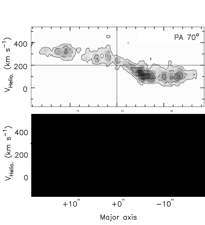
The total H92$\alpha$ line distribution extends over $\sim 35^{\prime\prime}$ along the major axis of M82 (Fig  5), covering the inner plateau and also the inner edges of the outer plateau. Since the resulting velocity field provides the average velocity value of the gas at each position, we have used the data cube to search for the steepest velocity gradient in the center of M82. The steepest velocity gradient is determined from terminal velocities ($\sim 36$ km s^-1 arcsec^-1) and is found along a PA of $\sim 57^{\circ}$. Only two regions, separated by $\sim 7\hbox to0.0pt{.\hss}{{}^{\prime\prime}}8$, define this velocity gradient: one of these regions is Ca and the other is a region located $0\hbox to0.0pt{.\hss}{{}^{\prime\prime}}4$ from W1c. The center defined by these two regions is located $1\hbox to0.0pt{.\hss}{{}^{\prime\prime}}7$ E from the 2.2 $\micron$ peak determined by Dietz et al. (1986). The velocity gradient could be alternatively defined between the region Ca and a region located near the center of E1a; in this case a velocity gradient of $\sim 27$ km s^-1 arcsec^-1, at a PA of $\sim 68^{\circ}$ is obtained. This PA agrees with the major axis of M82 determined on large scale. The position at mid-distance between these two regions (separated by $\sim 10^{\prime\prime}$) has an offset of $\Delta_{\alpha}=-1\hbox to0.0pt{.\hss}{{}^{\prime\prime}}5$, $\Delta_{\delta}=0\hbox to0.0pt{.\hss}{{}^{\prime\prime}}4$ relative to the 2.2 $\micron$ peak (Dietz et al., 1986). This offset corresponds approximately to the distance between the 2.2 $\micron$ peak and the center of the inner plateau observed in the $2.2~{}\micron$ profile (see Fig. 2 of Larkin et al. 1994). This asymmetry, with a truncation of the inner bar on the E side of the $2.2~{}\micron$ profile, has already been noticed by Larkin et al. (1994) and could reveal the presence of ionized gas in two lobes; this suggestion is supported by our H92$\alpha$ observations since the regions Ca and E1a appear as the only significant features in the channels at 313 and 284 km s^-1. Although different velocity gradients are obtained using the regions near E1a and W1c, both regions are located on the ridge of extinction determined by Larkin et al. (1994). In any case, the center position defined by these two regions is very close to the location of maximum extinction along this ridge. Dust lanes are expected to be present at the intersection of x1 and x2 orbits. This result suggests the presence of elongated x2 orbits. Assuming that the PA of the x1 orbits corresponds to the outer plateau is $\sim 70^{\circ}$ (Telesco et al., 1991), the major axis of the x2 orbits would be close to an end-on view.

The position-velocity (p-v) diagram, using the integrated flux density along the minor axis direction by taking slices at a PA of 70^∘, is shown in Figure 10 (top). This PA was used in order to compare with results from [Ne II] and Br$\gamma$ observations (Achtermann and Lacy, 1995; Larkin et al., 1994). In the H92$\alpha$ line image there is emission at “forbidden” velocities (near $-1\hbox to0.0pt{.\hss}{{}^{\prime\prime}}8$ at 215 km s^-1), inconsistent with purely circular motions. If non-circular motions are present, additional velocity components are observed. This feature is also observed in the $Br\gamma$ line images (Fig. 5 of Larkin et al. 1994). In [Ne II], there is also emission at “forbidden” velocities but this is distributed in a symmetrical fashion about 200 km s^-1 around the 2.2 $\micron$ peak. The agreement of the H92$\alpha$ p-v image is closer to the $Br\gamma$ (Larkin et al., 1994) p-v images than to the [Ne II] p-v image.

Figure 10 (bottom) shows the p-v image constructed along the major axis using the PA of $65^{\circ}$. In this case the profiles are in general relatively narrower when they are compared with those in Fig. 10 (top); the binning along the minor axis is over a smaller region of $\sim 1\hbox to0.0pt{.\hss}{{}^{\prime\prime}}5$ as compared with $9^{\prime\prime}$. However, the spectra remain relatively broad except near $8^{\prime\prime}$ on the W side and $10^{\prime\prime}$ on the E side. These two regions are located at the transition zones between the inner and outer 2.2 $\micron$ plateaus. The asymmetry observed at $2^{\prime\prime}$ angular resolution, relative to the position of the $2.2~{}\micron$ peak, is still present for this PA=65^∘, suggesting that the asymmetry is very likely to arise in the bar itself. In this case, there is no emission at “forbidden” velocities, indicating that the orbits must be confined to a relatively thin plane not observed edge-on. By comparing with optical measurements (McKeith et al., 1993; Greve et al., 2002), we observe systematic effects: in the inner part ($\leq 6^{\prime\prime}$) the terminal H92$\alpha$ velocities are close to the optical velocities only on the W side. Neither the gas nor the stars, as observed in the optical, have velocities near $\sim 325$ km s^-1 from $+1^{\prime\prime}$ to $+6^{\prime\prime}$. On the other hand, there are no optical velocities near $\sim 200$ km s^-1 from $-1^{\prime\prime}$ to $-6^{\prime\prime}$. Beyond $\pm 11^{\prime\prime}$, on the outer 2.2 $\micron$ plateau, the optical velocities are systematically closer to the low velocity component of the H92$\alpha$ profiles. These results would indicate that for the regions located in the outer plateau, the gas as well as the stellar emission observed in the optical comes preferentially from the leading edge of the bar in the x1 orbits (see Fig. 2 of Greve et al. 2002).

The symmetry observed in the terminal velocities of the H92$\alpha$ line would indicate that the component of the ionized gas that we observe is not only in the x1 orbits but also in x2 orbits ($\leq\pm 3^{\prime\prime}$) and/or with some “spraying” (at radial distances from $3^{\prime\prime}$ to $6^{\prime\prime}$). The result of gas shocking in the intersection of x1 and x2 orbits is named by some authors as “spray” orbits (e.g. Downes et al. 1996). The encounter of gas moving in these two orbits breaks the flow along the x1 orbit into a spray that traverses interior of the bar until it reaches the far side of the bar. A schematic diagram for these spray orbits is shown by Downes et al. (1996). In this context it is difficult to explain why the optical velocities are close to the H92$\alpha$ terminal velocities only on the W side. One possibility would be that the gas observed in the optical does not spray on the E side and the gas emitting the H92$\alpha$ line has orbits with radii which extend relatively closer to the nucleus. An alternate possibility would be that the x2 orbits are in a plane closer to $81^{\circ}$ inclination than the x1 orbits, the far side of the x2 orbits emitting in the optical being more severely affected by the extinction from dust in the plane of the x1 orbits.

There is a thin transition edge between the inner and outer plateaus not only observed in the p-v images made along the major axis (Fig. 10) but also in the velocity dispersion image (Fig. 8b). In Figure 8b an ellipse (fitted through the regions with local minima) is shown. This ellipse is centered at the same position as the ring found by Achtermann and Lacy (1995), with a major axis of $17^{\prime\prime}$ at a PA of 72^∘ and the same axial ratio of $\sim$3.5. This result agrees with the 2.2 $\micron$ light distribution for the inner plateau, consistent with a picture in which the inner and outer plateaus correspond to different families of orbits.

5.3.2 The inner ring.

A description in terms of elongated x1 and x2 orbits is not the only model that can explain the observed kinematics in M82. The observed velocities distribution is not consistent with a rotating disk unless it consists of a set of rings with different tilt angles which may be contracting. Different methods to fit a ring in the center of M82 were used; the results are listed in Table 6. Row 1 of Table 6 lists the results of Achtermann and Lacy (1995), column 1 lists the central position of the ring, column 2 the position angle of the major axis, columns 3 and 4 the angular size of the major and minor axis, column 5 the systemic velocity, column 6 the rotation velocity, column 7 the expansion velocity, column 8 the dispersion about the model and column 9 the spectral line used to obtain the parameters of the ring. Achtermann and Lacy (1995) fixed the geometry of the ring based on the physical appearance of the distribution of the [Ne II] line emission and then fitted the velocity pattern along that ring, assuming that the ring lies in the plane of the galaxy, centered on the kinematical center. Row 2 is the result obtained from the H92$\alpha$ velocity pattern (Fig. 8a), using the same morphological parameters listed in row 1. Following the same procedure for the H92$\alpha$ line emission, the ellipse fitted by Achtermann and Lacy (1995) would need to be shifted $\sim 0\hbox to0.0pt{.\hss}{{}^{\prime\prime}}3$ to the N (Fig. 4) to coincide with the ridge of emission. In row 3, this shift of $0\hbox to0.0pt{.\hss}{{}^{\prime\prime}}3$ has been applied. In row 4, the position of the center is a free parameter. Finally, row 5 lists the parameters of the ring (shown in Fig. 4) obtained without imposing any morphological constraints; this procedure gives the solution with the lowest residual dispersion.

Based on the spatial distribution of the line emission, the existence of the ring is not obvious in any of the models presented in Table 6. According to the ring model of Achtermann and Lacy (1995) and the one described by row 5 (Table 6), the rotation velocity $V_{rot}$ has a first maximum at a radius of $\sim 5^{\prime\prime}-6^{\prime\prime}$. In the model of Achtermann and Lacy (1995) the ring surrounds a region devoid of ionized gas, in contrast with the model presented here (the best fit to the velocity pattern). Both models require not only a contraction velocity but also that the inclination angle of the rings is different than the inclination of the plane of the outer part of M82 (i=$81^{\circ}$). The major axis of these rings is very close to the PA determined from the large scale morphology (68^∘).

In the velocity dispersion image (Fig. 8b), a well defined band at a PA of $\sim 150^{\circ}$ is observed with systematically narrower line profiles. The length of this band is not restricted to the extent of the minor axis of the ring with axial ratio of $\sim 3.5$ (Achtermann and Lacy, 1995); in addition this band covers the extent of the velocity pattern along that direction. On both sides of this band, there is a ridge in which the broadest profiles are observed. These regions of large velocity dispersions are explained by the terminal velocities V_t with $|$V${}_{t}-V_{sys}|\simeq 120$ km s^-1, along with a second velocity component in the spectra with velocities closer to V_sys, $|$V${}_{t}-V_{sys}|\simeq 50$ km s^-1. Figure 11 shows the p-v diagram along the E ridge. The regions where V_t $\geq+300$ km s^-1 are not restricted to the range $\leq\pm 1\hbox to0.0pt{.\hss}{{}^{\prime\prime}}7$, which corresponds to the regions associated with the ring of axial ratio of $\sim$3.5 (see Table 6). Outside the range $-5^{\prime\prime}$ to $+3^{\prime\prime}$, i.e. beyond the ring of axial ratio 2 (see Table 6), the bright component remains confined near $\sim 250$ km s^-1. We conclude that, if gas in x2 orbits and/or a fast rotating nuclear ring (spray between the x1 and x2 orbits) is responsible for V${}_{t}>+300$ km s^-1, it cannot be confined in a thin plane which would give this axial ratio of $\sim 3.5$.

5.3.3 Outflow in the halo.

Fig. 11 shows that for offsets larger than $-5^{\prime\prime}$ there is emission at two different velocities, one component emerging near $\sim 150$ km s^-1 and the second one near $\sim 350$ km s^-1. At $\sim-10^{\prime\prime}$ the emission is detected in the range $\sim 250$ km s^-1 and $\sim 30-100$ km s^-1. These results agree with the optical measurements (McKeith et al., 1993) in the lines of [SII], [NII], H$\alpha$. A more detailed view of the radial velocities of the outflow, observed in H$\alpha$, are shown in Figure 10 of Shopbell et al. (1998). The H92$\alpha$ observations reveal the base of the outflow into the halo. On the N side of M82 there are two velocity components: the ionized gas on the far side of the cone (component I) has radial velocities $\sim 250$ km s^-1 and on the near side of the cone (component II) the gas has radial velocities in the range $\sim 30$ to $100$ km s^-1. On the S side ($\sim+5^{\prime\prime}$), the velocities are confined to $\sim 200$ km s^-1 (component IV), again in agreement with the optical measurements (Shopbell et al., 1998). The geometry of the outflow and description of these four components are shown in Figure 5 of McKeith et al. (1995).

Due to the high inclination of M82, it is difficult to distinguish between an ad-hoc model of circular motions with radial contraction vs elliptical x1/x2 orbits. The ring models indicate contraction instead of expansion velocities (Table 6). The presence of different velocity components in the H92$\alpha$ line emission along a PA of $150^{\circ}$ indicates that the ionized gas near the nucleus has already been perturbed by the outflow. A barred potential seems to provide the mechanism to bring gas from the outer parts of the disk of M82 into the central part. In this way, the gas flowing into the center of M82 would be consumed in the starburst with some gas outflow into the halo.

5.4 Existence of an AGN

The presence of an AGN in the center of M82 has been proposed by Matsumoto & Tsuru (1999) based on X-ray data. These authors suggest that there is an under-luminous AGN in the center of M82, comparable to Sgr A^∗. In the continuum at 8.3 GHz (Fig. 2a), we observe a source located near the 2.2 $\mu$m peak (Lester et al., 1990). In the continuum at 43 GHz, we do not detect this source above the 3$\sigma_{rms}$ level. Muxlow et al. (1994), using MERLIN observations at 5 GHz with angular resolution of 50 mas, report a compact source (43.55+60.0) that was identified as a young supernova remnant with shell-like structure. Thus, no clear evidence has been found for the existence of a compact radio source that can be associated with an AGN in the center of M82 within our 8.3 GHz $3\sigma_{rms}$ limit of 0.12 mJy beam^-1.

6 CONCLUSIONS.

We have presented high angular resolution ($<1^{\prime\prime}$) VLA observations of radio continuum emission from M82 at 8.3 and 43 GHz and of the H92$\alpha$ and H53$\alpha$ RRLs. In the radio continuum images, we identified 19 new compact sources at 8.3 GHz and five at 43 GHz. Of these newly identified sources, four are SNRs, four are HII regions and the nature of the remaining 13 is uncertain. Three SNRs show the presence of H92$\alpha$ RRL emission which can be interpreted as line emission produced by HII regions along the line of sight. No compact source is observed near the position of the derived kinematic center. Thus, in agreement with Muxlow et al. (1994), we find that there is no compelling evidence for the existence of an AGN at the center of M82.

We have modeled the line and continuum emission using a collection of HII regions. We have considered models with a single density as well as models with two density components. The H53$\alpha$ RRL mainly traces the high-density ionized gas. Models with multiple HII regions were used to reproduce the observations in the continuum at 5, 8.3 and 43 GHz as well as the H92$\alpha$ and H53$\alpha$ RRL emission from four separate HII complexes. The two-density model is considered to be more appropriate to model the line and continuum emission since compact continuum sources have been identified already as HII regions. However, as the two-density model is based on previous identification of thermal compact sources, the emission from region E1 (no compact thermal sources have been identified) has been modeled using only the single-density model. In general the low-density component is characterized by HII regions with sizes of $\sim$0.8 pc and an average electron density of $\sim 5\times 10^{3}$ cm^-3 and the high-density component is characterized by HII regions with typical sizes of $\sim 0.15$ pc and an average electron density of $\sim 3.5\times 10^{4}$ cm^-3. From the two-density model, we can infer that the starburst in the region W1 is the youngest. The derived mass of ionized gas in the central region of M82 is $\sim 2\times 10^{8}$ M_⊙, 30 times lower than for Arp 220 (Anantharamaiah et al., 2000). Based on the models, it has been inferred that M82 has a star formation rate of $\sim 3$ M_⊙ year^-1, a factor $\sim$ 100 lower compared with the merging system Arp 220. For a more accurate determination of the properties of the ionized gas over a complete density range, high-resolution observations of RRLs at additional higher and lower frequencies are required.

The H92$\alpha$ line emission extends over $\sim 35^{\prime\prime}$. The steep velocity gradient, measured at PA of 68^∘, is 26 km s^-1 arcsec^-1 in the inner $\sim$100 pc of M82. At a distance of $\sim$80 pc from the kinematic center, the gas has a maximum radial velocity of $\sim$150 km s^-1, implying an enclosed total dynamical mass of $\sim$10⁸ M_⊙. From the p-v diagram of the H92$\alpha$ line, we observe deviations from circular motions. The observed velocity pattern cannot be due to pure circular motions; apparently the orbits in the inner parts of M82 are more face-on than in the outer parts. In the velocity dispersion image, the H92$\alpha$ line traces the base of a large scale outflow into the halo. This outflow is observed only on the N side. We find the PA of the axis of the outflow to be 150^∘. Along this axis, the widths of the profiles are narrow, suggesting collimated flow with small opening angle in the regions within the disk. Within the disk, the steepest gradient ($\sim 36$ km s^-1 arcsec^-1), is measured from the terminal velocities. This gradient is observed at a PA of $\sim 57^{\circ}$, in a direction perpendicular to the axis of the outflow into the halo. This direction is not parallel to the PA of the large scale major axis of M82 ($\sim 65^{\circ}$) nor the PA of the 2.2 $\micron$ bar ($\sim 70^{\circ}$).

The best fit with an ad hoc model of circular orbits leads to a contracting ring that has its kinematic center shifted $\sim 1^{\prime\prime}$ W of the 2.2 $\micron$ peak and located approximately in the middle of the 2.2 $\micron$ inner plateau. The nodes characterizing this ring coincide with the dust lanes; this coincidence could represent additional evidence of gas in x2 orbits of a bar potential. Due to the presence of the outflow, the kinematics observed in the H92$\alpha$ line provide possible evidence for the presence of x2 orbits originating from a bar potential. The inner and outer 2.2 $\micron$ plateaus correspond to two different families of orbits; the transition zone between the two plateaus has a signature in the kinematics in the form of a reverse in the velocity gradient that has been observed near the major axis.

The National Radio Astronomy Observatory is a facility of the National Science Foundation operated under cooperative agreement by Associated Universities, Inc. We thank J. M. Torrelles for making available his H92$\alpha$ data. We also thank Yolanda Gómez and anonymous referee for their very useful comments. CR acknowledges the support from UNAM and CONACyT, México.

Table 1: PARAMETERS OF THE VLA OBSERVATIONS OF M82

Parameter	H92$\alpha$ Line	H53$\alpha$ Line
Right ascension (B1950)	09h51m42$\hbox to0.0pt{.\hss}{{}^{s}}$38	09h51m42$\hbox to0.0pt{.\hss}{{}^{s}}$51
Declination (B1950)	69∘54′59$\hbox to0.0pt{.\hss}{{}^{\prime\prime}}$2	69∘55′00$\hbox to0.0pt{.\hss}{{}^{\prime\prime}}$0
Total observing duration (hr)	32	13
Bandwidth (MHz)	25	50$\times$2
Number of spectral channels	31	15$\times$2
Center VHel (km s-1)	200	160
Velocity coverage (km s-1)	700	350$\times$2
Velocity resolution (km s-1)	56	44
Amplitude calibrator	3C286	3C286
Phase calibrator	1044+719	0954+658
Bandpass calibrator	3C48	1226+023
RMS line noise per channel (mJy/beam )	0.07	1.3-2.0
RMS, continuum (mJy/beam )	0.04	0.5

Table 2: CONTINUUM FLUX DENSITIES, COMPACT FEATURES.

	8.3 GHz				43 GHz
Source ID1	Coordinates1	Size2	S8.3		Coordinates1	Size2	S43	Spectral index		RRL	Type
		(′′)	(mJy)			(′′)	(mJy)	8.3-43 GHz	Low freq.	feature
(1)	(2)	(3)	(4)		(5)	(6)	(7)	(8)	(9)	(10)	(11)
37.54+53.2	37.54+53.2a	0.5g	0.43$\pm$0.03		$-$	$-$	$<$1.5	$<$0.74	$-$	$-$
38.76+53.4	38.75+53.5b	0.5g	0.24$\pm$0.07		$-$	$-$	$<$1.5	$<$1.1	0.54$\pm$0.27d	$-$	HIIf
39.10+57.3	39.11+57.3b	u	3.81$\pm$0.04		$-$	$-$	$<$1.5	$<-$0.55	$-$0.53$\pm$0.09d	$-$	SNRf
39.29+54.2	39.27+54.1b	0.4	3.6$\pm$0.1		39.25+54.1b	0.5	3.5$\pm$0.3	$-$0.02$\pm$0.02	1.64$\pm$0.16d	$-$	HIIf
39.40+56.1	39.43+55.9b	0.5	1.9$\pm$0.1		$-$	$-$	$<$1.5	$<-$0.14	$-$1.04$\pm$0.22d	$-$	SNRf
39.64+53.4	39.65+53.2b	u	1.0$\pm$0.05		$-$	$-$	$<$1.5	$<$0.24	$-$0.20$\pm$0.05c	$-$	SNRf
39.68+55.6	39.67+55.3b	0.4	3.9$\pm$0.2		39.66+55.4b	0.5	3.6$\pm$0.5	$-$0.05$\pm$0.09	1.03$\pm$0.09d	$-$	HIIf
39.77+56.9	39.78+56.9b	0.4	0.7$\pm$0.05		$-$	$-$	$<$1.5	$<$0.45	$-$0.50$\pm$0.06c	$-$	SNRf
39.92+55.9	39.92+55.9a	0.7	2.7$\pm$0.1		$-$	$-$	$<$1.5	$<-$0.35	$-$	$-$	SNR?e
40.10+55.0	40.15+54.5b	0.7	0.6$\pm$0.05		$-$	$-$	$<$1.5	$<$0.54	$-$	$-$
40.32+55.1	40.33+55.1b	0.4	0.8$\pm$0.04		$-$	$-$	$<$1.5	$<$0.37	$-$0.23$\pm$0.21d	$-$	SNRf
40.49+57.4	40.49+57.4a	1.0	2.7$\pm$0.1		$-$	$-$	$<$1.5	$<-$0.35	$-$	$-$	SNR?e
40.62+56.0	40.63+56.0b	0.5	1.7$\pm$0.1		$-$	$-$	$<$1.5	$<-$0.01	$-$0.72$\pm$0.25d	$-$	SNRf
40.66+55.2	40.67+55.1b	0.4	5.6$\pm$0.1		40.65+55.1b	0.5	2.7$\pm$0.1	$-$0.43$\pm$0.05	$-$0.54$\pm$0.08d	$-$	SNRf
40.95+58.8	40.93+58.7b	0.5	4.5$\pm$0.4		40.92+58.7b	0.5	3.9$\pm$0.2	$-$0.09$\pm$0.06	0.44$\pm$0.13d	W2h	HIIf
40.96+57.9	40.96+57.8b	u	2.3$\pm$0.2		40.96+57.6b	0.5	1.8$\pm$0.1	$-$0.15$\pm$0.05	$>$1.2+	$-$	HIIf
41.17+56.2	41.17+56.1b	0.4	5.4$\pm$0.2		41.16+56.2b	0.7	4.9$\pm$0.4	$-$0.06$\pm$0.03	0.87$\pm$0.14d	W2f	HIIf
41.29+59.7	41.33+59.2b	0.7	3.0$\pm$0.2		$-$	$-$	$<$1.5	$<-$0.41	$-$0.47$\pm$0.09d	W2e	SNRf
41.62+59.9	41.62+59.9a	0.5	1.6$\pm$0.1		$-$	$-$	$<$1.5	$<-$0.04	$-$	$-$
41.95+57.5	41.95+57.4b	u	13.6$\pm$0.4		41.95+57.5b	0.7	5.0$\pm$0.1	$-$0.60$\pm$0.02	$-$0.80$\pm$0.05c	$-$	SNR?f
42.08+58.4	42.11+58.3b	0.4	4.0$\pm$0.2		42.09+58.3b	0.5	3.6$\pm$0.2	$-$0.06$\pm$0.04	1.32$\pm$0.17d	$-$	HIIf
42.21+59.0	42.20+59.0b	0.5	6.7$\pm$0.1		42.21+59.0b	0.7	6.5$\pm$0.3	$-$0.02$\pm$0.03	1.16$\pm$0.13d	W1f	HIIf
42.67+55.6	42.67+55.5b	u	0.92$\pm$0.04		$-$	$-$	$<$1.5	$<$0.29	$-$1.3$\pm$0.2d	$-$	SNRf
42.69+58.2 $\lceil$									$\rceil$ 1.04$\pm$0.13	W1c	HIIf
42.56+58.0 $|$	42.64+57.9b	$\sim 1.4$	32.4$\pm$0.7		42.64+57.9b	$\sim 1.2$	16.2$\pm$0.8	$-$0.41$\pm$0.2	$|$ 0.88$\pm$0.14	W1c	HIIf
42.48+58.4 $\lfloor$									$\rfloor$    $>$1.2	W1c	HIIf
43.00+59.0	43.02+58.9b	0.4	3.9$\pm$0.2		$-$	$-$	$<$1.5	$<-$0.56	$-$	W1a	SNR?e
43.18+58.3	43.17+58.3b	u	5.5$\pm$0.1		$-$	$-$	$<$1.5	$<-$0.77	$-$0.44$\pm$0.08d	$-$	SNRf
43.21+61.3	43.21+61.3a	0.8	4.3$\pm$0.1		43.25+61.4a	1.3	4.0$\pm$0.3	$-$0.04$\pm$0.05	$-$	$-$	HII?e
43.31+59.2	43.29+59.0b	u	8.0$\pm$0.2		43.30+59.2b	0.4	2.0$\pm$0.2	$-$0.83$\pm$0.06	$-$0.65$\pm$0.07d	$-$	SNRf
43.39+62.6	43.39+62.6a	0.7	7.0$\pm$0.2		43.39+62.7a	0.8	3.9$\pm$0.2	$-$0.34$\pm$0.14	$-$	Cd
43.50+61.2	43.50+61.2a	0.5	2.2$\pm$0.1		$-$	$-$	$<$1.5	$<-$0.23	$-$	$-$
43.55+60.0	43.57+59.8b	0.4	0.77$\pm$0.05		$-$	$-$	$<$1.5	$<$0.40	$-$	$-$
43.65+57.7	43.65+57.7a	0.7	2.3$\pm$0.1		$-$	$-$	$<$1.5	$<-$0.25	$-$	$-$
44.01+59.6	44.02+59.5b	0.4	19.5$\pm$0.2		44.01+59.5b	0.4	4.5$\pm$0.4	$-$0.87$\pm$0.05	$-$0.38$\pm$0.06d	$-$	SNRf
44.08+63.1	44.08+63.1a	0.8	4.1$\pm$0.1		$-$	$-$	$<$1.5	$<-$0.60	$-$	$-$
44.11+64.3	44.11+64.3a	0.5	2.1$\pm$0.1		$-$	$-$	$<$1.5	$<-$0.20	$-$	$-$	SNR?e
44.17+64.4	$-$	$-$	$<0.24$		44.17+64.4a	0.8	4.1$\pm$0.2	$>1.74$	$-$	$-$	HIIe
44.29+59.3	44.28+59.3b	u	2.3$\pm$0.1		$-$	$-$	$<$1.5	$<-$0.25	$-$0.72$\pm$0.12d	$-$	SNRf
44.36+57.8	44.36+57.8a	0.4	1.5$\pm$0.1		$-$	$-$	$<$1.5	$<$0.0	$-$	$-$
44.43+62.5	$-$	$-$	$<0.24$		44.43+62.5a	0.9	5.5$\pm$0.2	$>1.91$	$-$	E1b	HIIe
44.50+65.3	44.50+65.3a	0.5	1.4$\pm$0.1		$-$	$-$	$<$1.5	$<$0.0	$-$	$-$
44.52+58.1	44.52+58.0b	0.4	2.1$\pm$0.05		$-$	$-$	$<$1.5	$<-$0.20	$-$0.15$\pm$0.17d	$-$	SNRf
44.84+61.8	44.84+61.8a	u	0.95$\pm$0.05		$-$	$-$	$<$1.5	$<$0.27	$-$	$-$
44.91+61.1	44.89+61.2b	u	1.2$\pm$0.1		$-$	$-$	$<$1.5	$<$0.13	$-$0.45$\pm$0.18d	$-$	SNRf
44.93+63.9	44.92+63.7b	0.7	3.6$\pm$0.1		$-$	$-$	$<$1.5	$<-$0.52	$>$1.1d	E2f	HIIf
45.17+61.2	45.19+61.1b	0.4	6.7$\pm$0.1		$-$	$-$	$<$1.5	$<-$0.89	$-$0.52$\pm$0.07d	$-$	SNRf
45.38+60.3	45.38+60.3a	0.4	1.1$\pm$0.05		$-$	$-$	$<$1.5	$<$0.19	$-$	$-$
45.44+67.3	45.44+67.3b	0.4	1.47$\pm$0.06		$-$	$-$	$<$1.5	$<$0.0	$-$	$-$
45.63+66.9	45.63+66.9a	0.8	5.8$\pm$0.2		45.61+67.1a	0.9	5.5$\pm$0.4	$-0.04$	$-$	E2c	HIIe
45.70+62.9	45.66+62.8b	0.4	0.78$\pm$0.05		$-$	$-$	$<$1.5	$<$0.39	$-$	$-$
45.79+65.2	45.74+65.5b	0.5	5.9$\pm$0.2		$-$	$-$	$<$1.5	$<-$0.81	$-$0.55$\pm$0.13d	E2b	SNRf
45.91+63.8	45.88+63.7b	0.4	1.28$\pm$0.05		$-$	$-$	$<$1.5	$<$0.01	$-$0.38$\pm$0.11d	$-$	SNRf
45.93+74.3	45.93+74.3a	1.0	1.4$\pm$0.1		$-$	$-$	$<$1.5	$<$0.01	$-$	$-$
46.17+67.6	46.17+67.6b	0.8	4.6$\pm$0.1		46.21+67.8b	0.8	4.5$\pm$0.3	-0.02$\pm$0.04	0.66$\pm$0.16d	E2a	HIIf
46.33+66.2	46.33+66.2a	u	0.93$\pm$0.05		$-$	$-$	$<$1.5	$<$0.28	$-$	$-$
46.52+63.8	46.53+63.9b	0.4	2.1$\pm$0.1		$-$	$-$	$<$1.5	$<-$0.20	$-$0.35$\pm$0.11d	$-$	SNRf
46.56+73.8	46.57+73.7b	u	0.76$\pm$0.05		$-$	$-$	$<$1.5	$<$0.40	$-$0.60$\pm$0.05c	$-$	SNRf
46.74+69.7	46.74+69.7a	1.4	4.3$\pm$0.2		$-$	$-$	$<$1.5	$<-$0.63	$-$	$-$	SNR?e
46.75+67.0	46.69+66.9b	0.4	1.8$\pm$0.1		$-$	$-$	$<$1.5	$<$0.11	$-$0.80$\pm$0.05c	$-$	SNRf
47.11+66.3	47.11+66.3a	0.5	1.12$\pm$0.05		$-$	$-$	$<$1.5	$<$0.17	$-$	$-$
47.37+68.0	47.37+67.8b	0.4	0.7$\pm$0.05		$-$	$-$	$<$1.5	$<$0.45	$-$0.60$\pm$0.07c	$-$	SNRf

Table 3: LINE PARAMETERS AT LOW ANGULAR RESOLUTION USED IN THE MODELS.

	H92$\alpha$					H53$\alpha$
Region	Peak Flux	VHEL	$\Delta$V	SC8		Peak Flux	VHEL	$\Delta$V	SC43	ffb	SC5
	(mJy)	(km/s)	(km/s)	(mJy)		(mJy)	(km/s)	(km/s)	(mJy)	(10-3)	(mJy)
E2	2.2$\pm$0.1	315$\pm$2	106$\pm$5	106$\pm$10		7.5$\pm$1.5	305$\pm$5	55$\pm$12	46$\pm$17	1.3	152
E1	1.0$\pm$0.1	269$\pm$3	130$\pm$8	72$\pm$10		6.7$\pm$1.5	264$\pm$5	50$\pm$13	28$\pm$15	$--$	93
W1	6.4$\pm$0.1	119$\pm$1	116$\pm$3	292$\pm$15		9.8$\pm$2.0	113$\pm$12	120$\pm$29	157$\pm$20	3.2	403
W2	4.2$\pm$0.1	100$\pm$2	112$\pm$4	169$\pm$15		10.2$\pm$2.0	66$\pm$9	100$\pm$22	101$\pm$19	6.8	230

Table 4: PARAMETERS FOR REGIONS OBSERVED IN H92$\alpha$ RRL

	Low angular resolution			Intermediate resolution
Region	$\int$SLdV	SL/S${}_{C}^{a}$	Features	Coordinatesb	$\int$SLdV	Sizec	Peak Flux	VHEL	$\Delta$V${}^{d}_{FWHM}$
	(mJy km $s^{-1}$)	($\times 10^{-2}$)			(mJy km $s^{-1}$)	$(^{\prime\prime})$	(mJy)	(km/s)	(km/s)
(1)	(2)	(3)	(4)	(5)	(6)	(7)	(8)	(9)	(10)
E2	604	1.7$\pm$0.1	E2a	46.20+67.7	81	1.3	0.57$\pm$0.03	316$\pm$16	121$\pm$37
			E2b	45.79+65.3	65	1.4	0.82$\pm$0.05	315$\pm$5	48$\pm$11
			E2c	45.54+66.3	165	1.6	1.54$\pm$0.14	320$\pm$8	84$\pm$19
			E2d	45.43+65.6	96	0.8	0.82$\pm$0.05	311$\pm$5	95$\pm$11
			E2e	45.32+64.2	69	0.9	0.61$\pm$0.05	314$\pm$5	90$\pm$11
			E2f	45.05+63.5	32	0.4	0.26$\pm$0.06	302$\pm$7	102$\pm$16
			E2a+E2b+…+E2f		508
E1	300	1.2$\pm$0.1	E1a	44.39+61.8	98	1.4	0.87$\pm$0.07	264$\pm$8	90$\pm$18
			E1b	44.10+62.7	56	1.6	0.56$\pm$0.05	321$\pm$10	76$\pm$24
			E1c	44.02+60.3	39	1.4	0.59$\pm$0.05	231$\pm$10	24$\pm$24
			E1a+E1b+E1c		193
C	320	1.0$\pm$0.1	Ca	43.84+62.4	70	0.9	0.63$\pm$0.05	300$\pm$5	88$\pm$11
			Cb	43.77+63.2	137	1.2	0.61$\pm$0.05	286$\pm$5	205$\pm$11
			Cc	43.79+63.9	16	0.6	0.30$\pm$0.05	470$\pm$5	52$\pm$11
			Cd	43.39+62.3	75	1.3	1.00$\pm$0.05	239$\pm$4	44$\pm$9
			Ca+Cb+Cc+Cd		298
W1	1067	1.6$\pm$0.1	W1a	42.95+59.2	85	1.9	0.72$\pm$0.10	165$\pm$8	96$\pm$4
			W1b	42.62+60.3	196	2.1	1.85$\pm$0.10	148$\pm$3	83$\pm$8
			W1c	42.61+58.0	291	1.7	2.88$\pm$0.07	117$\pm$2	77$\pm$3
			W1d	42.32+61.5	57	1.1	0.56$\pm$0.10	191$\pm$8	78$\pm$4
			W1e	42.21+59.9	147	1.3	1.05$\pm$0.07	125$\pm$2	120$\pm$3
			W1f	42.19+58.8	177	1.6	2.01$\pm$.10	100$\pm$3	61$\pm$8
			W1a+W1b+…+W1f		953
W2	878	2.0$\pm$0.1	W2a	41.75+59.0	113	1.4	0.76$\pm$0.07	114$\pm$12	128$\pm$32
			W2b	41.62+57.8	141	u	1.43$\pm$0.07	79$\pm$12	69$\pm$32
			W2c	41.51+58.6	81	1.2	0.68$\pm$0.07	113$\pm$3	96$\pm$6
			W2d	41.47+56.6	69	1.6	0.80$\pm$0.08	76$\pm$5	57$\pm$12
			W2e	41.27+59.2	65	1.1	0.69$\pm$0.11	135$\pm$5	68$\pm$10
			W2f	41.12+56.4	113	1.8	1.19$\pm$0.08	86$\pm$5	69$\pm$12
			W2g	41.07+61.0	36	1.3	0.23$\pm$0.07	84$\pm$3	133$\pm$6
			W2h	40.97+58.5	112	1.4	1.14$\pm$0.09	129$\pm$4	73$\pm$9
			W2a+W2b+…+W2h		730

Table 5: MODELS BASED ON THE H92$\alpha$ AND H53$\alpha$ LINES

Parameter	Region E2		Region E1	Region W1		Region W2
	SD	TD	SD	SD	TD	SD	TD
T${}_{e}\times 10^{3}$ (K)	7$\pm$2	$\big{\{}$$7.5\pm 2.5\atop 6\pm 1$	7.5$\pm$2.5	6$\pm$0.5	$\big{\{}$$7.5\pm 2.5\atop 5\pm 0.5$	7.5$\pm$2.5	$\big{\{}$$7.5\pm 2.5\atop 6\pm 1$
n${}_{e}\times 10^{3}$(cm-3)	9$\pm$8	$\big{\{}$$40\pm 20\atop 5\pm 4$	26$\pm$25	4$\pm$3	$\big{\{}$$30\pm 10\atop 4.0\pm 2.5$	15$\pm$13	$\big{\{}$$30\pm 10\atop 5.5\pm 4.0$
Size (pc)	0.81$\pm$0.59	$\big{\{}$$0.14\pm 0.05\atop 0.85\pm 54$	0.75$\pm$0.65	0.72$\pm$0.34	$\big{\{}$$0.15\pm 0.04\atop 0.73\pm 33$	0.52$\pm$0.36	$\big{\{}$$0.15\pm 0.04\atop 0.69\pm 0.38$
N${}_{HII}\times 10^{3}$	2.5$\pm$1.0	$\big{\{}$$0.56\pm 0.35\atop 2.4\pm 1.1$	1.7$\pm$0.88	5.8$\pm$1.1	$\big{\{}$$1.6\pm 0.7\atop 4.6\pm 0.3$	6.8$\pm$3.8	$\big{\{}$$2.4\pm 1.0\atop 4.6\pm 2.6$
f	0.29$\pm$0.28	$\big{\{}$$0.0013\atop 0.29\pm 0.27$	0.27$\pm$0.26	0.31$\pm$0.24	$\big{\{}$$0.0032\atop 0.30\pm 0.23$	0.37$\pm$0.35	$\big{\{}$$0.0068\atop 0.40\pm 0.37$
Log NLy (s-1)	52.36$\pm$0.19	$\big{\{}$$51.64\pm 0.32\atop 52.33\pm 0.21$	52.16$\pm$0.25	52.75$\pm$0.09	$\big{\{}$$52.15\pm 0.2\atop 52.67\pm 0.03$	52.75$\pm$0.27	$\big{\{}$$52.34\pm 0.2\atop 52.58\pm 0.27$
SFR (M⊙ year-1)	0.37$\pm$0.13	$\big{\{}$$0.10\pm 0.07\atop 0.45\pm 0.19$	0.21$\pm$0.11	1.64$\pm$0.13	$\big{\{}$$0.29\pm 0.13\atop 0.86\pm 0.05$	0.63$\pm$0.51	$\big{\{}$$0.45\pm 0.19\atop 0.86\pm 0.48$
$\tau_{c}$ (8.3 GHz)	0.27$\pm$0.26	$\big{\{}$$0.032\pm 0.023\atop 0.14\pm 0.13$	0.51$\pm$0.50	0.10$\pm$0.08	$\big{\{}$$0.015\pm 0.007\atop 0.09\pm 0.07$	0.35$\pm$0.32	$\big{\{}$$0.015\pm 0.007\atop 0.14\pm 0.12$
$\tau_{L}$ (8.3 GHz)	$-0.13\pm 0.10$	$\big{\{}$$-0.050\pm 0.048\atop-0.095\pm 0.068$	$-0.16\pm 0.13$	$-0.09\pm 0.05$	$\big{\{}$$-0.032\pm 0.027\atop-0.085\pm 0.042$	$-0.14\pm 0.11$	$\big{\{}$$-0.051\pm 0.047\atop-0.095\pm 0.068$
bn (H92$\alpha$)	0.97$\pm$0.02	$\big{\{}$$0.92\pm 0.03\atop 0.96\pm 0.02$	0.97$\pm$0.03	0.97$\pm$0.02	$\big{\{}$$0.91\pm 0.025\atop 0.97\pm 0.014$	0.98$\pm$0.02	$\big{\{}$$0.91\pm 0.025\atop 0.97\pm 0.02$
$\beta_{n}$ (H92$\alpha$)	$-20\pm$15	$\big{\{}$$-23\pm 8.1\atop-22\pm 13$	$-20\pm$16	$-19\pm$9	$\big{\{}$$-26\pm 5\atop-20\pm 8$	$-18\pm$12	$\big{\{}$$-26\pm 5\atop-20\pm 11$
$\alpha$	0.95$\pm$0.20	$1.0\pm 0.24$	1.00$\pm$0.30	0.50$\pm$0.03	$0.52\pm 0.026$	0.91$\pm$0.5	$0.62\pm 0.19$
M${}_{HII}\times 10^{4}$ (M⊙)	2.5$\pm$2.6	$\big{\{}$$0.041\pm 0.008\atop 3.0\pm 2.6$	1.5$\pm$1.4	6.6$\pm$4.5	$\big{\{}$$0.16\pm 0.02\atop 6.1\pm 4.0$	5.6$\pm$5.1	$\big{\{}$$0.25\pm 0.03\atop 6.1\pm 5.4$

Table 6: MODELS FOR A NUCLEAR RING.

Ring center   b	PA   b	Maj   b	Min   b	Vsys   b	Vrot   b	Vexp   b	$\sigma_{fit}$	Line
	(deg.)	(arcsec)		(km s-1)
9h51m43$\hbox to0.0pt{.\hss}{{}^{s}}$40, 69∘55′0$\hbox to0.0pt{.\hss}{{}^{\prime\prime}}$1b	70	11.4	3.3	200	112	-16		[Ne II]a
9h51m43$\hbox to0.0pt{.\hss}{{}^{s}}$40, 69∘55′0$\hbox to0.0pt{.\hss}{{}^{\prime\prime}}$1b	70	11.4	3.3	193	94	-13.5	7.47	H92$\alpha$
9h51m43$\hbox to0.0pt{.\hss}{{}^{s}}$40, 69∘55′0$\hbox to0.0pt{.\hss}{{}^{\prime\prime}}$4b	70	11.4	3.3	196	96	-15	7.27	H92$\alpha$
9h51m43$\hbox to0.0pt{.\hss}{{}^{s}}$19, 69∘55′0$\hbox to0.0pt{.\hss}{{}^{\prime\prime}}$6	70	11.4	3.3	191	102	-13	7.35	H92$\alpha$
9h51m43$\hbox to0.0pt{.\hss}{{}^{s}}$28, 69∘55′0$\hbox to0.0pt{.\hss}{{}^{\prime\prime}}$6	66	11.4	5.6	195	103	-14	4.82	H92$\alpha$

Figure 1: a) Radio continuum images at 8.3 GHz made with the VLA in the B and C arrays. Contour levels are drawn at -3, 3, …, 269 times the rms noise of 0.07 mJy beam^-1 at steps of 2^1/2. The gray scale covers the range from 0 to 70 mJy beam^-1. b) Radio continuum images at 43 GHz made in the C array of the VLA. Contour levels are -3, 3, 4, 6, 8, 10 times 0.4 mJy beam^-1, the rms noise in the central regions. The gray scale image covers the range from 3 mJy beam^-1 to 53 mJy beam^-1. In both images, the radio continuum made with high angular resolution of $0\hbox to0.0pt{.\hss}{{}^{\prime\prime}}6$ (contours) is superposed on the radio continuum image with low angular resolution of $2^{\prime\prime}$ (gray scale). The square shows the position of the 2.2 $\micron$ peak (Lester et al., 1990) and the circle marks the position of the SNR G41.95+57.5.

Figure 2: Radio continuum images after subtracting the background local emission. (a) 8.3 GHz image (B and C arrays). Contour levels are -3, 3, 6, 12, 24, 48, 96 times the rms noise of 0.04 mJy beam^-1. (b) 43 GHz image (C array). Contour levels are drawn at -3, 3, 4, 6, 8, 10 times the rms noise of 0.4 mJy beam^-1. Both images have angular resolution of $0\hbox to0.0pt{.\hss}{{}^{\prime\prime}}6$. The crosses (+) indicate the position of SNRs, while the rotated crosses (X) indicate the HII regions (McDonald et al., 2002). The empty squares show the position of sources previously observed, for which the spectral index has not been determined. The empty circle marks the position of the 2.2 $\mu$m peak (Lester et al., 1990). The newly detected features are labeled according to their positions (e.g. 39.92+55.9).

Figure 3: High angular resolution images of the H92$\alpha$ line emission (contours) throughout the velocity region where emission was observed in the central region of M82. The beam size is $0\hbox to0.0pt{.\hss}{{}^{\prime\prime}}6$, shown in the bottom left corner of the first image. The contour levels are -3, 3, 4, 5, 6 times the rms noise of $\sim$0.12 mJy beam^-1. The central heliocentric velocity is given above each image. The cross (+) indicates the position of the compact source 43.00+59.0, classified in this work as SNR (see discussion in section 5), and the rotated crosses (X) indicate the HII regions; all of these are compact sources observed in the continuum (McDonald et al., 2002; Huang et al., 1994) and coincide with features observed in the H92$\alpha$ line.

Figure 4: Top) Contour images of the H92$\alpha$ line intensity throughout the velocity region where emission was observed at intermediate-resolution ($0\hbox to0.0pt{.\hss}{{}^{\prime\prime}}9$). The contour levels are $-$3, 3, 4, 5, 6, 7, 8, 9 times the rms noise of $\sim$0.07 mJy beam^-1. The integrated line emission obtained from the low-resolution ($2^{\prime\prime}$) line images is shown in gray scale. The gray scale image covers the range from 0 to 6 Jy beam^-1 m s^-1. The marks indicate the position of the HII regions (crosses) and the SNRs (stars). The central heliocentric velocity is given above each image. The beam size is shown in the bottom left corner of the first image. Bottom) Integrated H92$\alpha$ line emission at $0\hbox to0.0pt{.\hss}{{}^{\prime\prime}}9$ angular resolution toward M82. Contour levels are 0.4, 0.8, 1.2, 1.6, 2.0 mJy beam^-1 km s^-1. The cross indicates the 2.2 $\mu$m peak (Lester et al., 1990). The outer ellipse shows the extension of the inner 2.2 $\micron$ plateau. The ellipses shown correspond to models of Table 6 in row 1 and 5, respectively.

Figure 5: Top) Contour images of the H92$\alpha$ line at low angular resolution ($2^{\prime\prime}$). The contour levels are $-$3, 3, 5, 7, 9, 11, 13, 15, 17, 19 times the rms noise of $\sim$0.07 mJy beam^-1. The filled circle shows the position of G41.95+57.5 and the filled square the peak at 2.2 $\mu$m (Lester et al., 1990). The beam size is shown in the bottom left corner of the first image. Bottom) Integrated H92$\alpha$ line emission at $2^{\prime\prime}$ angular resolution toward M82. Contour levels are from 15.82 up to 158.2 by increment of 15.82 mJy beam^-1 km s^-1. The two line segments show the minor and major axis of a thin disk which would be observed with an inclination of 81^∘ and centered at the position of the 2.2 $\mu$m peak (Dietz et al., 1986). The cross indicates the 2.2 $\mu$m peak (Lester et al., 1990).

Figure 6: a) The integrated H92$\alpha$ line emission (contours) superposed on the radio continuum at 8.3 GHz (gray-scale) at $2^{\prime\prime}$ angular resolution. Contour levels are drawn at 18 through 148 mJy beam^-1 km s^-1 in steps of 26 mJy beam^-1 km s^-1. The gray scale for the continuum covers the range from 5.4 to 55 mJy beam^-1. b) The integrated H53$\alpha$ line emission (contours) superposed on the radio continuum image of M82 at 43 GHz (gray-scale) at $2^{\prime\prime}$ angular resolution. Contour levels are at 57, 114, 171, 228, 285 Jy beam^-1 km s^-1. The gray scale for the continuum covers the range from 2.3 to 34 mJy beam^-1. c) Integrated intensity of H92$\alpha$ line (gray-scale) and integrated intensity image of the H53$\alpha$ line (contours). Contour levels are 57, 114, 171, 228 Jy beam${}^{-1}~{}$ km s^-1. The gray scale covers the range from 8.4 to 196 mJy beam^-1 km s^-1. The square marks the position of the 2.2 $\micron$ peak (Lester et al., 1990) and the circle marks the position of the SNR G41.95+57.5.

Figure 7: H92$\alpha$ and H53$\alpha$ spectra toward the regions labeled in Figure 6c. The dashed curves are the observed intensities and the solid lines represent the fitted gaussians as a function of heliocentric velocity.

Figure 8: a) H92$\alpha$ velocity field at $2^{\prime\prime}$ angular resolution. Contour intervals are 16 km s^-1, the iso-velocity contours $\geq$ 200 km s^-1 are in black. b) Spatial distribution for the velocity dispersion of the H92$\alpha$ profiles. The contours from 15 to 35 km s^-1 are in black and above this level in white. The contour interval is 5 km s^-1. The most elongated ellipse is a fit to a ridge with minimum velocity dispersion which corresponds to the transition between the inner and outer plateau in the 2.2 $\micron$ brightness distribution. In both images, the less elongated ellipse corresponds to the model of row 5 (Table 6). The two perpendicular line segments are the same as in Figure 5 (bottom). The cross indicates the center of the ring fitted by Achtermann and Lacy (1995).

Figure 9: Expected variation of radio continuum (left) and integrated line flux density (right) for four of the regions identified in Fig. 6c. The continuum flux density has been computed using the model of multiple HII regions with a single component plus non-thermal emission arising from SNR. The integrated line emission curves correspond to the single-density models of Table 5.

Figure 10: H92$\alpha$ position-velocity diagram summed over the minor axis (angular resolution $0\hbox to0.0pt{.\hss}{{}^{\prime\prime}}9$), along: top) the main axis of the stellar bar with PA$=$70^∘. Contours are from 0.3 to 3.0 in steps of 0.6 mJy beam^-1, and bottom) the major axis of M82 determined on larger scales with PA$=$65^∘. Small circles marks the velocity of the stars as determined from [Ca II] line (McKeith et al., 1993) and big circles show the velocity of the gas determined in Pa(10) line (McKeith et al., 1993). Contours are 0.1, 0.4 and 1.5 mJy beam^-1. The beam is $2\hbox to0.0pt{.\hss}{{}^{\prime\prime}}5\times 0\hbox to0.0pt{.\hss}{{}^{\prime\prime}}9$. The gray scales follow the contours. The slices were centered at $\alpha$=09^h51^m43$\hbox to0.0pt{.\hss}{{}^{s}}6$, $\delta$=69${}^{\circ}55^{\prime}00^{\prime\prime}$.

Figure 11: Position-velocity image along the E ridge of broad profiles (see Fig. 8) at 150^∘. The angular resolution is $0\hbox to0.0pt{.\hss}{{}^{\prime\prime}}9$. The offsets are relative to the major axis, NW to the left and SE to the right, the origin being at $\alpha=$09^h51^m43$\hbox to0.0pt{.\hss}{{}^{s}}$81, $\delta=$69^∘55^′1$\hbox to0.0pt{.\hss}{{}^{``}}$1. Contours are -0.1, -0.05 mJy beam^-1 (dashed) and from 0.05 to 0.5 mJy beam^-1 in steps of 0.05 mJy beam^-1.

References

- Achtermann and Lacy (1995) Achtermann, J. M. & Lacy, J. H., 1995, ApJ, 439, 163
- Allen & Kronberg (1998) Allen, M. L. & Kronberg, P. P., 1998, ApJ, 502, 218
- Anantharamaiah et al. (2000) Anantharamaiah, K. R., Viallefond, F., Mohan, N. R., Goss, W. M. & Zhao, J.H., 2000, ApJ, 537, 613
- Anantharamaiah & Goss (1996) Anantharamaiah, K. R. & Goss, W. M., 1996, ApJ, 466, L13
- Anantharamaiah et al. (1993) Anantharamaiah, K. R., Zhao, Jun-Hui, Goss, W. M. & Viallefond, F., 1993, ApJ, 419, 585
- Anantharamaiah & Goss (1990) Anantharamaiah, K. R. & Goss, W. M., 1990, Radio Recombination Lines: 25 Years of Investigation, ed: M. A. Gordon and R. L. Sorochenko, Kluwer Academic Publishers, 267
- Bartel et al. (1987) Bartel, N., Ratner, M. I., Rogers, A. E. E., Shapiro, I. I., Bonometti, R. J., Cohen, N. L., Gorenstein, M. V., Marcaide, J. M., & Preston, R. A., 1987, ApJ, 323, 505
- Bell & Seaquist (1978) Bell, M. B., & Seaquist, E. R., 1978, ApJ, 223, 378
- Chaisson & Rodríguez (1977) Chaisson, E. J., & Rodríguez, L. F., 1977, ApJ, 214, L111
- Colbert et al. (1999) Colbert, J. W. et al., 1999, ApJ, 511, 721
- Dietz et al. (1986) Dietz, R. D., Smith, J., Hackwell, J. A., Gehrz, R. D., & Grasdalen, G. L., 1986, AJ, 91, 758
- Downes et al. (1996) Downes, D., Reynaud D., Solomon, P. M., & Radford, S. J. E., 1996, ApJ, 461, 186
- Garay & Rodríguez (1983) Garay, G. & Rodríguez, L. F., 1983, ApJ, 266, 263
- Greve et al. (2002) Greve, A., Wills, K. A., Neininger, N., & Pedlar, A., 2002, A&A, 383, 56
- Huang et al. (1994) Huang, Z. P., Thuan, T. X., Chevalier, R. A., Condon, J. J., & Yin, Q. F., 1994, ApJ, 424, 114
- Kronberg et al. (1985) Kronberg, P. P., Biermann, P., & Schwab, F. R., 1985, ApJ, 291, 693
- Larkin et al. (1994) Larkin, J. E., Graham, J. R., Matthews, K., Soifer, B. T., Beckwith, S., Herbst, T. M., Quillen, A. C., 1994, ApJ, 420, 159
- Lester et al. (1990) Lester, D. F., Gaffney, N., Carr, J. S., & Joy, M., 1990, ApJ, 352, 544
- Matsumoto & Tsuru (1999) Matsumoto, H., & Tsuru, T. G., 1999, PASJ, 51, 321
- Matsushita et al. (2000) Matsushita, S., Kawabe, R., Matsumoto, H., Tsuru, T. G., Kohno, K., Morita, K., Okumura, S. K., & Vila-Vilarbo, B., 2000, ApJ, 545, 107
- McDonald et al. (2002) McDonald, A. R, Muxlow, T. W. B., Wills, K. A., Pedlar, A., & Beswick, R., 2002, MNRAS, 334, 912
- McKeith et al. (1993) McKeith, C. D., Castles, J., Greve, A., & Downes, D., 1993, A&A, 272, 98
- McKeith et al. (1995) McKeith, C. D., Greve, A., Downes, D., Prada, F., 1995, A&A, 293, 703
- Mohan et al. (2002) Mohan, N. R., Anantharamaiah, K. R., & Goss, W. M., 2002, ApJ, 574, 701
- Muxlow et al. (1994) Muxlow, T. W. B., Pedlar, A., Wilkinson, P. N., Axon, D. J., Sanders, E. M., & de Bruyn, A. G., 1994, MNRAS, 266, 455
- Rodríguez et al. (1980) Rodríguez, L. F., Moran, J. M., Gottlieb, E. W., & Ho, P. T. P., 1980, ApJ, 235, 845
- Roelfsema (1987) Roelfsema, P. R., 1987, PhDT, Univ. Groningen, 126
- Salem & Brocklehurst (1979) Salem, M., & Brocklehurst, M., 1979, ApJS, 39, 633
- Schraml & Mezger (1969) Schraml, J., & Mezger, P. G., 1969, ApJ, 156, 269
- Seaquist & Bell (1977) Seaquist, E. R.,& Bell, M. B., 1977, A&A, 601, 1
- Seaquist et al. (1985) Seaquist, E. R., Bell, M. B.,& Bignell, R. C., 1985, ApJ, 294, 546
- Seaquist et al. (1996) Seaquist, E. R., Carlstrom, J. E., Bryant, P. M., & Bell, M. B., 1996, ApJ, 465, 691
- Shopbell et al. (1998) Shopbell, P.L., Bland-Hawthorn, J., 1998, ApJ 493, 129
- Telesco et al. (1991) Telesco, C. M., Joy, M., Dietz, K., Decher, R., Campins, H., 1991, ApJ, 369, 135
- Weiss et al. (1999) Weiss, A., Walter, F., Neininger, N., Klein, U., 1999, A&A, 345, 23
- Wills et al. (1997) Wills, K. A., Pedlar, A., Muxlow, T. W. B., & Wilkinson, P. N., 1997, MNRAS, 291, 517
- Wills et al. (2000) Wills, K. A., Das, M., Pedlar, A., Muxlow, T. W. B., & Robinson, T. G., 2000, MNRAS, 316, 33
- Zhao et al. (2000) Zhao, J. H., Goss, W. M., Ulvestad, J., & Anantharamaiah, K. R., ASP Conference Series, 2000
- Zhao et al. (1996) Zhao, J. H., Anantharamaiah, K. R., Goss, W. M., & Viallefond, F., 1996, ApJ, 472, 54