CHORIZOS: a CHi-square cOde for parameteRized modelIng and characteriZation of phOtometry and Spectrophotometry

Abstract

We have developed a CHi-square cOde for parameteRized modelIng and characteriZation of phOtometry and Spectrophotometry (CHORIZOS). CHORIZOS can use up to two intrinsic free parameters (e.g. temperature and gravity for stars; type and redshift for galaxies; or age and metallicity for stellar clusters) and two extrinsic ones (amount and type of extinction). The code uses $\chi^{2}$ minimization to find all models compatible with the observed data in the model $N$-dimensional ($N=1,2,3,4$) parameter space. CHORIZOS can use either correlated or uncorrelated colors as input and is especially designed to identify possible parameter degeneracies and multiple solutions. The code is written in IDL and is available to the astronomical community. Here we present the techniques used, test the code, apply it to a few well-known astronomical problems, and suggest possible applications. As a first scientific result from CHORIZOS, we confirm from photometry the need for a revised temperature-spectral type scale for OB stars previously derived from spectroscopy.

1 Introduction

A general problem in astronomy is that of finding the correspondence between the observed spectrophotometric and/or photometric properties and a series of models parameterized in terms of physical quantities. Perhaps the best well-known example is the utilization of Johnson $U-B$ and $B-V$ colors to measure the temperature and extinction of main-sequence stars (see, e.g. Binney & Merrifield 1998) but the problem appears in a variety of contexts, such as the calculation of photometric redshifts with optical/IR photometry (Koo, 1999; Benítez, 2000), of extinction laws using a combination of UV-to-IR spectroscopy and photometry (Cardelli et al., 1989; Fitzpatrick, 1999), or of stellar cluster ages and metallicities using broad-band colors (Girardi, 2000; Whitmore et al., 1999; de Grijs et al., 2003). Each one of those cases has its own specific peculiarities, but they can all be considered as examples of the following general problem. A family of spectral energy distribution (SED) models $f(\lambda;p_{1},p_{2}\ldots,p_{N})$ is generated as a function of $N$ parameters. Some of those parameters $p_{i}$ may depend on the nature and distance to the objects (e.g. temperature, age, metallicity, or redshift) while others depend on the properties of the intervening ISM (amount and type of extinction). The first type of parameters will be called in this paper intrinsic (to the object) and the second type extrinsic (to the object). Our data consists of one or several objects with measured magnitudes $m_{1},m_{2}\ldots m_{M+1}$ ($M\geq N$), each with its independent uncertainty $s_{1},s_{2}\ldots s_{M+1}$ from which we can derive $M$ independent colors $c_{1},c_{2}\ldots c_{M}$. The general problem can be then expressed as finding what model SEDs are compatible with the observed colors. The solution could be:

• Unique, if the observed values for the colors and their uncertainties determine a single set of connected SED models (i.e. a connected $N-$volume in $N-$dimensional parameter space) that can be described by a single set of parameters with their corresponding uncertainties.

• Multiple, if the provided colors do not allow to differentiate between two or more sets of connected SED models.

• Non-existent, if the properties of the object fall outside the parameter range of the SED models, the chosen SED models are an incorrect description of the object, or the photometry has systematic errors.

Several related codes are discussed in the literature (see e.g. Romaniello et al. 2002; Benítez 2000; de Grijs et al. 2003) but they all have one shortcoming: they are designed to deal only with an specific case of the general problem (stellar temperatures, photometric redhifts, cluster ages). Furthermore, some of the codes are discussed in an article but are not available to the astronomical community, thus hampering the testing of results by other groups. Finally, the treatment of how uncertainties in the measured quantities affect the derived parameters is in many cases poor or inexistent (some photometric redshift codes are an exception, see e.g. Benítez 2000).

We discuss in this paper CHORIZOS, a code that solves the general problem of identifying which models are compatible with an observed set of colors. In section 2 we analyze the problems that have to be dealt with and in section 3 we discuss the techniques to overcome them. In section 4 we apply an implementation of the algorithm to a number of cases and we end in section 5 with a summary.

2 Description

2.1 Problem definition

We start by defining two different cases as a function of the number of colors and parameters, $M=N$ and $M>N$. For $M=N$, we can establish as many equations (sets of model parameters that produce a given color) as unknowns (model parameters) and the problem can be treated as that of finding an exact solution to a (complicated) algebraic system of equations. Barring strict degeneracies in the system of equations, one can find either zero, one, or a finite number of solutions in $N-$dimensional parameter space depending on the specific topology of the $N-$volume defined in $M-$dimensional color space by all the possible parameter combinations. Adding the corresponding uncertainties associated with each color produces at least one connected $N-$volume around each of the solutions in parameter space and can also generate new $N-$volumes disconnected from any of the strict solutions and/or establish connections between solutions. For $M>N$, the problem has more equations than unknowns and no exact solutions should be expected. However, approximate solutions that are compatible with the measured uncertainties can still be found. In this case, our goal should be to find that $N-$volume of approximate solutions by using e.g $\chi^{2}$ minimization.

2.2 $M=N$: the main-sequence $B-V$ vs. $U-B$ example

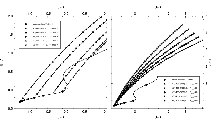
Figure 1: (left) $U-B$ vs. $B-V$ color-color plot for $Z=0.0$, main-sequence Kurucz atmospheric models. The line with circles indicates the location of the unredenned values as a function of temperature, starting at $T=50\,000$ K, with the circles marking those points where the temperature is a multiple of 5 000 K. The rest of the lines indicate the colors as a function of reddening using the Cardelli et al. (1989) law with $R_{5495}=3.1$ for five different temperatures. Symbols are plotted at intervals of $\Delta\mbox{$E(4405-5495)$}\ =0.1$0. (right) Same as left but now plotting colors as a function of reddening for five different values of $R_{5495}$ using the same family of extinction laws for a temperature of 50 000 K. The scale has been enlarged to include all unredenned models with $T=3\,500-50\,000$ K and all 50 000 K models up to $\mbox{$E(4405-5495)$}=5.0$.

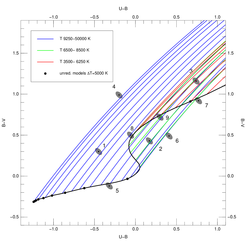
Figure 2: $B-V$ vs. $U-B$ color-color plot for the same conditions as in Fig. 1. Here we include a higher number of extinguished models using a color code to differentiate among temperature ranges which are relevant to determine the number of possible temperature + reddening solutions for a given $(U-B)$ + $(B-V)$ color combination. Nine examples are marked, each one of them with $\sigma_{U}=\sigma_{B}=\sigma_{V}=0.026$.

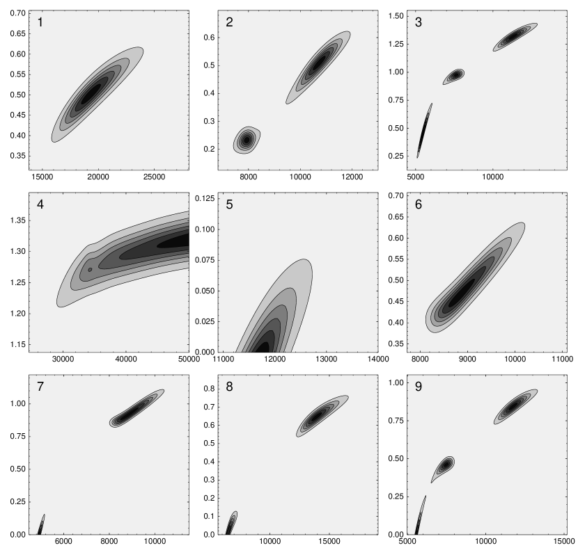
Figure 3: Likelihood contour plots produced by CHORIZOS for the nine examples described in the text and shown in Fig. 2. The $x$ axis corresponds to the temperature in K and the $y$ axis to $E(4405-5495)$.

Given the complexity and non-linearity of the general problem, different topologies can exist, leading to different solution types as a function of the measured magnitudes. In order to visualize them, we analyze the well-known example of using Johnson $U-B$ and $B-V$ colors to measure stellar temperature and reddening ($M=N=2$). We show in the left panel of Fig. 1 the locations in 2-D color space of unreddened main-sequence stars using as model atmospheres those of Kurucz (2004) with $Z=0.0$. The Kurucz atmospheres were extinguished using a Cardelli et al. (1989) law with $R_{5495}=3.1$ from $\mbox{$E(4405-5495)$}=0.0$ to 5.0; five different values of the temperature are shown. We also show in Fig. 2 a similar plot but with more temperature values (here some of the symbols have been omitted for clarity). Nine examples of measured magnitudes are shown in Fig. 2, each one of them with different measured magnitudes $U$, $B$, $V$, but with the same uncertainty $\sigma_{U}=\sigma_{B}=\sigma_{V}=0.026$ in each case. The corresponding solutions (as calculated by CHORIZOS) are shown in Fig. 3 as likelihood contour plots. The examples have been selected to reflect the different solution types.

• Example 1 is the ideal observational situation: the measured colors correspond to a unique solution and the inclusion of uncertainties leads to a single set of connected solutions around it. We can see that because the corresponding shaded area in Fig. 2 is crossed only by blue lines, which correspond to models with $T=9\,250-50\,000$ K and this leads to a single connected region in Fig. 3.

• Example 2 falls in a region where, due to the change in direction experienced by the zero-extinction color-color curve around $T=9\,000$ K, two different sets of connected solutions exist. Its shaded area in Fig. 2 is crossed by both blue and green lines and tracing them back to the zero-extinction case we arrive at two possible different ranges of values for the temperature.

• Example 3 falls in the region in Fig. 2 to the upper right from where the zero-extinction color-color curve has changed direction for the second time. As a result, the region is crossed by lines corresponding to three temperature ranges (represented in Fig. 2 in blue, green and red, respectively) and three different sets of connected solutions are possible. This translates into three peaks in Fig. 3.

• Examples 4, 5, and 6 correspond to the situation where the measured $U-B$ and $B-V$ colors are incompatible with any of the models but the inclusion of the corresponding uncertainties generates a single connected region in Fig. 3. In the case of examples 4 and 5, the nearest edge of the $N-$volume of allowed colors in Fig. 2 corresponds to an extreme in $N-$dimensional parameter space (maximum temperature - 50 000 K - for example 4, minimum $E(4405-5495)$ - 0.0 - for example 5). Therefore, the corresponding likelihood contour plots in Fig. 3 show abrupt edges. On the other hand, the nearest edge of the $N-$volume of allowed colors for example 6 does not correspond to such an extreme; instead, it is caused by the change in direction of the zero-extinction color-color curve around $T=9\,000$ K. Therefore, its likelihood contour plot does not show an abrupt edge.

• For example 7 the measured $U-B$ and $B-V$ values fall outside the $M-$volume of allowed colors but in this case there are two nearby boundaries, one of the same type as that of example 5 and another one of the same type as that of example 6. This translates into two peaks in Fig. 3, one with an abrupt edge and another one without it.

• Examples 8 and 9 correspond to the cases where at least one solution exists for the measured colors (one for example 8, two for example 9). Here, the inclusion of uncertainties not only generates a connected region around each one of them but also a new one, leading to the existence of two peaks in Fig. 3 for example 8 and of three peaks for example 9.

• Finally, though we have not plotted them, we can describe two possible additional situations. One would be the case where the shaded region in Fig. 2 was outside the $M-$volume of allowed colors and far from an edge. That would indicate that the data and the models are incompatible. Another situation would be reached by increasing the uncertainties in e.g. example 2. Then, we could have two possible solutions for the measured values of $U-B$ and $B-V$ but only a single set of connected solutions, since the shaded region in Fig. 2 would extend to the line defined by the turnaround point in temperature around 9 000 K.

We can group our examples as a function of their solution into the three categories described in the introduction: unique, multiple, and non-existent. It is important to differentiate between cases with unique and multiple solutions for the following reason. For unique solutions (e.g. example 1), the derived parameters can be correctly characterized by a single set of mean values, $\overline{T}$ and $\overline{\mbox{$E(4405-5495)$}}$, and a covariance matrix defined by $\sigma_{T}$, $\sigma_{E(4405-5495)}$, and $\sigma_{T,E(4405-5495)}$. In principle, one could do the same for multiple solutions (e.g. example 2), but that would not be a correct characterization, since in those cases there are two or more peaks in the likelihood contour plot. In those cases, given the strong deviations from a Gaussian distribution, it would be misleading to give mean parameter values, since those may fall in regions of very low probability while the main peaks may be located at distances around or above 1 $\sigma$ from them (see. e.g. example 2, where the mean values are $T=9\ 910$ K, $\mbox{$E(4405-5495)$}=0.383$, and the standard deviations $\sigma_{T}=1\,350$ K and $\sigma_{E(4405-5495)}=0.139$.

It is also important to note that, even in those cases where a unique solution is found, there is typically a strong correlation between the parameters. This is seen in Fig. 3 in that, if we were to approximate each peak by an ellipsoid, the two principal axes would be inclined with respect to the $x$ and $y$ axes. This effect is commonly referred to in the literature as a degeneracy between the two parameters. E.g., for example 6 we may say that $T$ and $E(4405-5495)$ are degenerate because our colors are compatible with a single set of connected solutions where likely deviations from the mean require either (a) an increase in both temperature and reddening or (b) a decrease in both, but not e.g. an increase in temperature and a decrease in reddening.

2.3 $M>N$ and solution existence

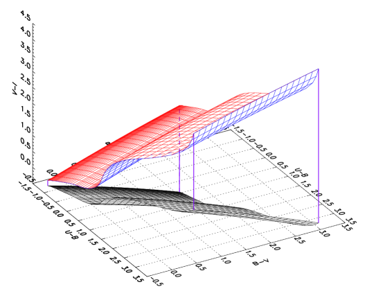
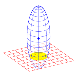
Figure 4: (left) $V-I$ vs. $B-V$ vs. $U-B$ 3-color plot for $Z=0.0$, main-sequence Kurucz atmospheric models. The range plotted covers $T=3\,500-50\,000$ and $\mbox{$E(4405-5495)$}=0.0-2.0$ and the extinction law used is that of Cardelli et al. (1989) with $R_{5495}=3.1$. The color surface marks the location in 3-color space while the black one is the projection onto the $(U-B)$-$(B-V)$ plane (see Figs. 1 and 2). (right) Basic topology for an $M=3$, $N=2$ case such as the one on the left panel. Given that $M>N$, the measured colors (blue circle) always lies outside the solution surface (red grid). However, including the uncertainty ellipsoid (blue grid), yields an intersection surface (solid yellow) of likely solutions.

The introduction of additional colors and parameters beyond two is straightforward if we keep $M=N$ (though not as easy to plot). Instead of dealing with the intersection between ellipses and regions of a plane, we have to find the intersection between $M-$ellipsoids and regions of an $N-$ (or $M-$) dimensional space, which does not introduce any new behavior from the topological point of view in our description. The situation is different if $M>N$. Take as an example $M=3$ and $N=2$. There, we have that the two available parameters generate a surface ($N-$volume) of possible solutions inside the volume ($M-$volume) of all possible color combinations. Given the difference in dimensions, a given set of three measured colors will always fall outside the solution surface. However, adding uncertainties to the measured colors will generate a finite ellipsoid ($M-$ellipsoid) in color space that, barring problems with the data or the models, should intercept the solution surface. This is represented on the right panel of Fig. 4 for the simple case where the solution surface is a plane perpendicular to the major axis of the uncertainty ellipsoid. For more complex solution surfaces, such as the one in the left panel of Fig. 4, the intersections can have more complex shapes but the topological classification into unique (one connected intersection surface), multiple (two or more intersection surfaces), and non-existent (no intersection) solution sets remains unchanged.

Therefore, for $M>N$ we cannot have strict solutions but only approximate ones. We can characterize those by defining $\chi^{2}$ for the case of uncorrelated uncertainties as:

$$\chi^{2}=\sum_{m=1}^{M}\frac{\left(c_{m}-c_{m,\rm mod}\right)^{2}}{\sigma_{m}^{2}},$$ (1)

where $c_{m,\rm mod}$ are the model colors and $\sigma_{m}$ the measured color uncertainties. For Gaussian uncertainties, the likelihood is then given by ${\cal L}=\exp(-\chi^{2}/2)$ and maximizing it is equivalent to finding the model(s) that minimize(s) $\chi^{2}$. It can be shown (see e.g. Gould 2003) that the expected value of $\chi^{2}_{\rm min}$ is $M-N$, with a standard deviation of $\sqrt{2(M-N)}$. Note that those are the results expected even for the case $M=N$, where we should find a model with the same exact colors as those measured and, therefore, have a $\chi^{2}_{\rm min}$ of exactly zero. Our definition of solution existence for $M>N$ would be to have a $\chi^{2}_{\rm min}$ reasonably close to $M-N$ in units of $\sqrt{2(M-N)}$.

An exception to the last statement should be noted. If the measured value lies close to an $(N-1)-$dimensional edge of the solution $N-$volume, then the value of $\chi^{2}_{\rm min}$ could be larger than $M-N$. An easy way to see this is with the most extreme case of $M=N$. In examples 4 to 7 of the previous section we saw that it is reasonable to have measured colors incompatible with the model ones if they fall just outside the edge of the region spanned by the models. In those situations where the data is close to such an edge, it is then normal to find somewhat higher values of $\chi^{2}_{\rm min}$: for the specific case $M=N$, one should then only reject the existence of a solution if $\mbox{$\chi^{2}_{\rm min}$}\gg 1$.

It is still possible to find data for which there are no solutions, either for the $M=N$ case or for the $M>N$ ones. The following is a checklist of possible causes, some general and some specific to astronomical photometry:

• Model validity: the models may be an incorrect description of the real SED.

• Model applicability: the type of object or the parameter range selected may be incorrect.

• Model approximations: make sure that you are deriving your colors the right way. Common errors are using the wrong extinction law and neglecting curvature effects in extinction trajectories for large values of $E(4405-5495)$ (see Fig. 1).

• Photometric quality: were the data properly acquired and calibrated?

• Zero-point calibration: some filters require small magnitude corrections before their magnitudes can be used for spectrophotometry (see e.g. Cohen et al. 2003).

• Filter-throughput errors: make sure that the throughputs of your filter are correctly characterized. Be on the alert for filters with red/blue leaks and long tails.

• Color transformations: beware of transforming from one filter system to another. Whenever possible, use the throughput definitions for the filters with which the data was acquired.

3 Techniques

Apparently, two different techniques should be needed to solve the two different cases defined in the previous section. In practice, both can be solved using a $\chi^{2}$ minimization algorithm. That is so because for $M=N$, the algebraic solution to the system of equations is also the solution that makes $\chi^{2}=0$, which is obviously the minimum possible value for $\chi^{2}$. Furthermore, since ${\cal L}=\exp(-\chi^{2}/2)$ independently of the number of degrees of freedom, we can use that definition to estimate the uncertainties in our parameters not only for $M>N$ but also for $M=N$.

CHORIZOS works by computing $\chi^{2}$ over the $N-$dimensional parameter grid and calculating the corresponding likelihood at each grid point. The current version of the code is written in IDL and handles up to $N=4$: two parameters from the intrinsic properties of the SED family plus two extinction-related parameters, $E(4405-5495)$ and extinction law type. The latter includes the $R_{5495}$-dependent family of extinction laws of Cardelli et al. (1989), the average LMC and LMC2 laws of Misselt et al. (1999), and the SMC law of Gordon & Clayton (1998). CHORIZOS starts by reading the unreddened SED models, extinguishing them, and obtaining the synthetic photometry at each point in a (coarse) 4-D grid. This is done in order to correctly deal with non-linear extinction effects. This preliminary step needs to be executed only once and the result can be stored in the form of binary FITS tables for later use. Currently, CHORIZOS includes pre-calculated tables for Kurucz (Kurucz, 2004), Lejeune (Lejeune et al., 1997), and TLUSTY (Lanz & Hubeny, 2003) stellar models and Starburst 99 (Leitherer et al., 1999) cluster models using a total of 78 filter passbands (including the Johnson, Strömgren, 2MASS, and several HST instrument systems). The two intrinsic parameters are temperature and gravity for the stellar models and age and metallicity for the cluster models. More models and passbands will be included in the future and the user will also be able to add his/her own.

The program first reads the photometry from a user-provided table, as well as a series of input parameters, such as which model family should be used and how fine a parameter grid should be employed. At this point, the user can restrict any of the four parameters for any of the objects (stars, clusters or galaxies) in the input table, using either a specific value or a range between a minimum and a maximum. CHORIZOS then reads the model photometry from the previously calculated tables and interpolates to the user-selected (fine) grid. For each object, the likelihood is calculated at each grid point, the average values of the four parameters and their (output) 4$\times$4 covariance matrix are computed, and the result is written in an individual file for each star. This file is read by a second program which produces the graphical output and allows for further manipulation of the results, such as calculation of stellar absolute magnitudes or cluster stellar masses.

There are several issues regarding algorithm details and results interpretation for a program of this type that need to be discussed. First, if one measures magnitudes directly and then calculates two different colors that include one filter in common (e.g. $B$ in the example discussed in the previous section), then the probability distributions for the two colors will be correlated (see, e.g. the data plotted in Fig. 2). It can be easily shown that for the case of the two colors $X-Y$ and $Y-Z$ formed from the three filters $X$, $Y$, and $Z$, the input (or color) covariance matrix is:

$${\cal C}_{X-Y,Y-Z}={\rm cov}(X-Y,Y-Z)=\left(\begin{array}[]{cc}\sigma_{X}^{2}+\sigma_{Y}^{2}&-\sigma_{Y}^{2}\\ -\sigma_{Y}^{2}&\sigma_{Y}^{2}+\sigma_{Z}^{2}\end{array}\right),$$ (2)

where $\sigma_{X}$, $\sigma_{Y}$, and $\sigma_{Z}$ are the uncertainties which correspond to each filter. For correlated uncertainties, Eqn. 1 is no longer valid and one has to use (see e.g. Gould 2003):

$$\chi^{2}=\sum_{l=1}^{M}\sum_{m=1}^{M}\left(c_{l}-c_{l,\rm mod}\right){\cal B}_{lm}\left(c_{m}-c_{m,\rm mod}\right),$$ (3)

where ${\cal B}\equiv{\cal C}^{-1}$, the inverse of the $M\times M$ input (or color) covariance matrix. Note, however, that in some cases two colors such as $U-B$ and $B-V$ can be considered to be in a first approximation as uncorrelated. That would be the case if those colors are built from the combination of a large number of independent measurements of $U-B$ and $B-V$, a situation that one may encounter when collecting data from the literature. CHORIZOS allows either option to be used: if individual magnitudes are inputted, then the full input covariance matrix is utilized; if colors are chosen, then only the corresponding diagonal terms are used. Given the relative complexity of the algorithm implementation, We conducted an independent test using a Montecarlo simulation in which the measured colors were varied according to the input covariance matrix and the solution that minimized $\chi^{2}$ was selected in each case. The Montecarlo simulation was run with 1000 samples and the results were combined to produce a likelihood map which was then compared to the CHORIZOS output using a variety of input data and models. Results agreed in all cases.

Another issue is that of grid size. When calculating the solution, CHORIZOS also checks whether the width of the resulting distribution in parameter space is comparable to that of the grid size near the optimum solution and warns the user if it finds that condition is not met so that a new run with a finer grid can be executed. A related issue is that of the value of $\chi^{2}_{\rm min}$ for the case $M=N$. As we have mentioned, it should be zero, unless the measured colors are incompatible with the models (e.g. the solution falls outside the $N-$volume of allowed colors). Therefore, the value of $\chi^{2}_{\rm min}$ can be used to check such a circumstance. Since we are using a grid to evaluate $\chi^{2}$, the minimum value will not be zero but if the grid is fine enough it should be $\ll 1$. But what if the grid is not fine enough? To solve this problem, after CHORIZOS finds the solution that minimizes $\chi^{2}$, it interpolates the colors from the adjacent points into an ultrafine grid in order to obtain a more accurate value of the minimum. This value can then be used to decide whether the measured colors fall outside the $N-$volume of allowed colors or not.

A problem also arises when the measured colors fall exactly at the edge of the $N$-volume of allowed colors. One example would be if in the temperature-reddening case using $U-B$ and $B-V$ the measured colors were to correspond to those of a star with zero reddening (the resulting likelihood diagram could be similar to that of example 5 in Fig. 3). In that case, the resulting mean reddening value from the likelihood data would be greater than zero and if we were to measure a number of stars with real $E(4405-5495)$ equal to zero, we would obtain positive values in all cases, leading us to an incorrect estimation of the value of the reddening. One solution which is implemented in CHORIZOS as an option is to extrapolate the grid to values beyond those provided by the original models. Using that option, the likelihood plot for example 5 in Fig. 3 would show the full ellipsoid and the correct mean value could be obtained (which in that specific case would be negative, given the location of point 5 in Fig. 2). This option should be used with caution, though, since extending the grid too much can easily lead to the inadvertent introduction of false additional solutions. Also, in some cases the use of extrapolated values is not recommended due to the existence of color near-degeneracies at the grid edges (e.g. the optical colors at the high-temperature end for O stars).

Finally, the validity of the derived mean values and covariance matrix when the calculated parameter distribution is far from being a Gaussian (e.g. when multiple solutions exist) has to be analyzed. We will do this in the following section, where we discuss some sample applications of CHORIZOS.

4 Sample applications

4.1 Multiple solutions for stars using Johnson-Cousins photometry

As we have seen, $U-B$ and $B-V$ colors alone are not enough to provide a single solution under all circumstances for main-sequence stellar atmospheres using a fixed extinction law. But what if we use additional filters in the Johnson-Cousins set? If we add the $I$ filter and use $V-I$ as a third color, we have the situation represented on the left panel in Fig. 4. We can see that in this case a third color eliminates most or all the multiple solutions. However, since we now have $M=3>N=2$, the problem does not have an exact solution for an arbitrary combination of colors and we are forced into using a $\chi^{2}$ minimization or a similar technique.

We analyze here a similar case using five Johnson-Cousins filters and a total of four colors: $U-B$, $B-V$, $V-R$, and $V-I$ to measure the temperature and reddening of a main-sequence star. We use $Z=0.0$, main-sequence Kurucz atmospheres, restrict the extinction law to be that of Cardelli et al. (1989) with $R_{5495}=3.1$, and fix the uncertainties in all five passbands to be 0.01 magnitudes. The grid was extrapolated in $E(4405-5495)$ but not in $T$. In order to compare the results obtained with the full $UBVRI$ photometry with those of only $UBV$ photometry, We ran CHORIZOS using its test mode. In that mode, CHORIZOS is fed the true model colors and is executed to see if it is able to reproduce them. If there is a single well-behaved solution, the measured mean parameters should be very similar to the input ones; if there are multiple solutions, that may not be the case. One way to quantify the effect is to use the mean calculated temperature and reddening, $\overline{T}$ and $\overline{\mbox{$E(4405-5495)$}}$, and their uncertainties estimated from their standard deviations, $\sigma_{T}$ and $\sigma_{E(4405-5495)}$, to calculate their normalized distances from the input value:

$$d_{T}=(\overline{T}-T_{\rm input})/\sigma_{T},$$ (4)

$$d_{E(4405-5495)}=(\overline{\mbox{$E(4405-5495)$}}-\mbox{$E(4405-5495)$}_{\rm input})/\sigma_{E(4405-5495)}.$$ (5)

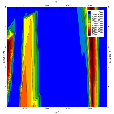
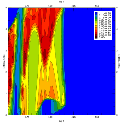
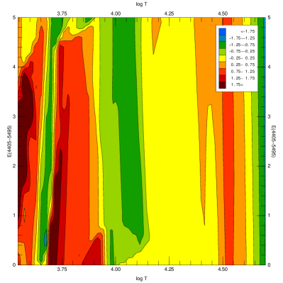
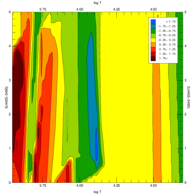
Figure 5: (top) Plots of $\sigma_{T}$ (left) and $\sigma_{E(4405-5495)}$ (right) for sample application 1 (main-sequence Kurucz models with $R_{5495}=3.1$) as a function of $\log T$ (in K) and $E(4405-5495)$ calculated for $UBV$ photometry with uncertainties of 0.01 magnitudes for each filter. (bottom) Plots of $d_{T}$ (left) and $d_{E(4405-5495)}$ (right) corresponding to the same case.

For a single well-behaved solution one expects low values of $\sigma_{T}$ and $\sigma_{E(4405-5495)}$ (unless the input uncertainties themselves are large) and, more importantly, values of $|d_{T}|$ and $|d_{E(4405-5495)}|<1.0$ (and typically lower than 0.5). If there are two or more solutions, the normalized distances can easily be larger than one because for such a distribution (formed by e.g. two well-separated narrow quasi-Gaussians) the maxima can be separated from the mean by more than one standard deviation. We have plotted those four quantities for the test case with only $UBV$ photometry in Fig. 5.

• For $T>15\,000$ K, CHORIZOS detects the existent unique solutions, as evidenced by the relatively low values of the uncertainties and absolute values of the normalized distances. Two minor points can be noted: the somewhat larger values of $\sigma_{T}$ around $37\,000$ K are caused by the near-degeneracy of the optical colors of O stars. Also, the green region at the right border of the normalized distance plots is caused by edge effects (we did not extrapolate in temperature).

• For $T<15\,000$ K, CHORIZOS produces in general much larger values of the uncertainties (especially for $E(4405-5495)$) and the normalized distances are of the order of or larger than one (in absolute value) for most of the region. This is caused by the existence of multiple solutions.

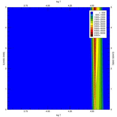
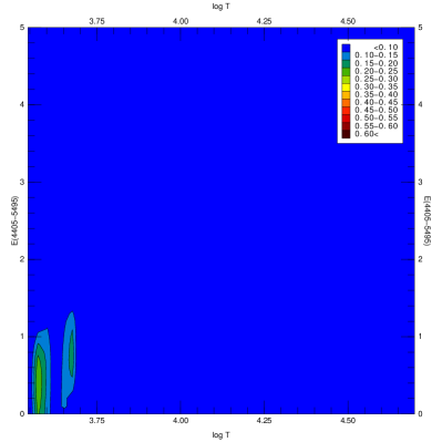
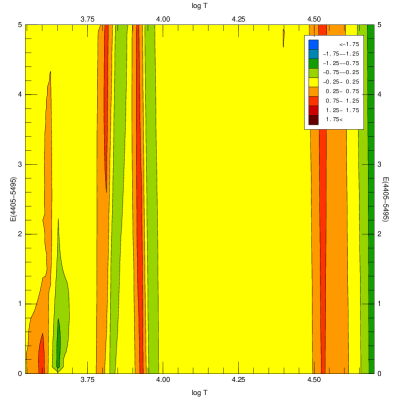
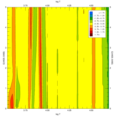
Figure 6: Same as Fig. 5 for $UBVRI$ photometry.

These results are simply what we expected. The interesting point is that this demonstrates that when CHORIZOS is run in test mode, it can be used to predict which parameter ranges can be measured with the existent colors and precisions and which ones cannot be measured. We now turn to Fig. 6, which has the same plots but for the test case with the full $UBVRI$ data using the same color scale.

• The values of the uncertainties are much lower, being $<500$ K and $<0.10$ for $\sigma_{T}$ and $\sigma_{E(4405-5495)}$, respectively, over most of the analyzed range. The only significant deviations are those for $\sigma_{T}$ around $T\approx 40\,000$ K, where the introduction of $RI$ data alleviates the color near-degeneracy but does not eliminate it completely, and for $\sigma_{E(4405-5495)}$ at certain regions near the lower left of the diagram; both effects are quite minor.

• The values of the normalized distances (in absolute value) are also much smaller, with only a few regions coming close to 1.0 (in some cases due to edge effects; see, however, the comparison below with Lejeune atmospheres)).

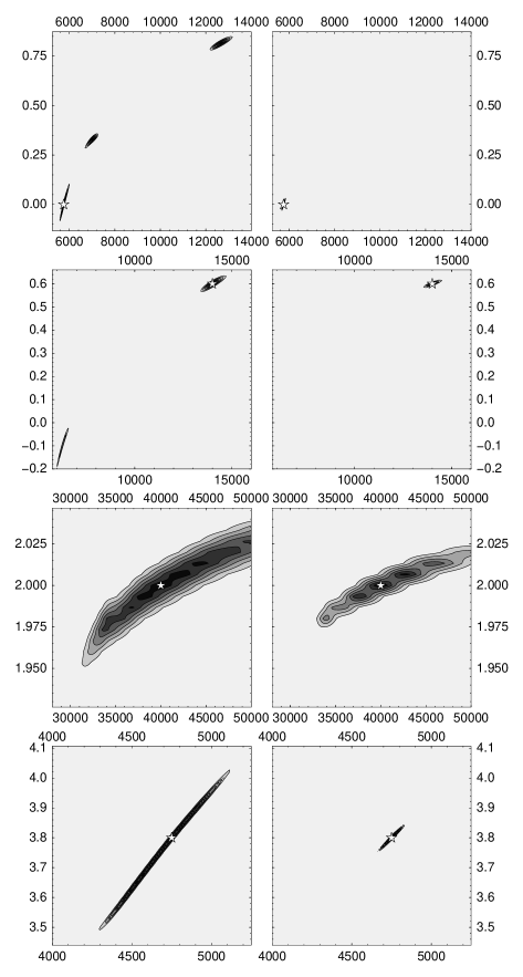
Figure 7: Likelihood contour diagrams for four selected cases in sample application 1 using $UBV$ data (left) and $UBVRI$ data (right). Temperature (in K) is plotted in the horizontal axis and $E(4405-5495)$ in the vertical axis. A white star is used to indicate the true temperature and reddening. The irregularities in the contour diagram for the third star are caused by grid-size effects.

• A comparison between the likelihood plots produced by CHORIZOS from $UBV$ and $UBVRI$ cases are shown in Figs. 7 and 8. The first of those two figures shows four examples where the introduction of $RI$ data yields excellent solutions, in some cases eliminating one of the multiple solutions and in others simply reducing the extent of the possible range of values. The second figure shows two of the cases where $|d_{T}|$ and $|d_{E(4405-5495)}|$ are close to 1.0 even for the $UBVRI$ case. We can see that, even in those “bad” cases, the introduction of $RI$ data is useful in further constraining the values of the parameters. The reasons for the high values of the normalized distances are, in one case, the persistence of two solutions (with a narrowing of each peak) and, in the other one, the reduction to a single solution with an asymmetrical distribution.

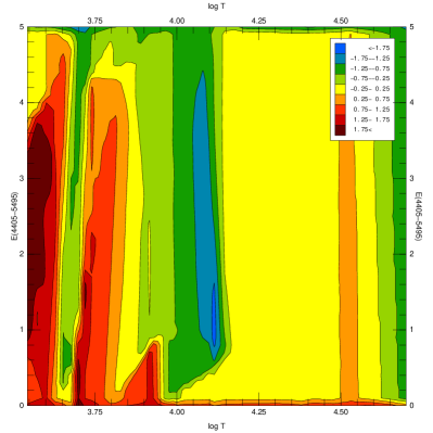
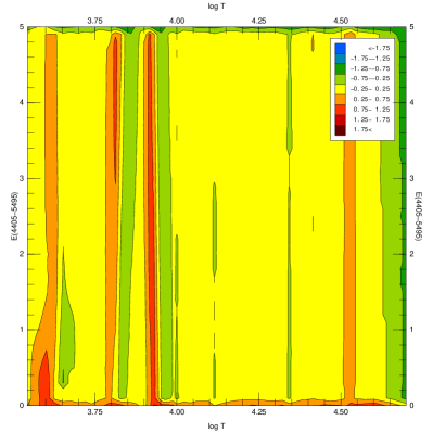
Figure 9: Plots of $d_{E(4405-5495)}$ for sample application 1 without grid extrapolation in $E(4405-5495)$ for the $UBV$ (left) and UBVRI (right) cases.

The importance of extending the grid for some parameters can be seen in Fig. 9, where we plot the values of $d_{E(4405-5495)}$ for two test runs identical to the ones just described with the only exception of not using the grid extension option. We see there how $|d_{E(4405-5495)}|$ is significantly larger around $\mbox{$E(4405-5495)$}=0.0$ and $\mbox{$E(4405-5495)$}=5.0$.

Table 1: FITMODEL temperature measurements from Johnson $UBVRI$ photometry.

Star	Spectral	Temperature			$\mbox{$\chi^{2}_{\rm min}$}/(M-N)$
	type	Reference	Kurucz	Lejeune	Kurucz	Lejeune
HD 36512	B0 V	29800	25989$\pm$0678	25990$\pm$0679	0.17	0.17
HD 37018	B1 V	26600	22704$\pm$0721	22707$\pm$0721	2.39	2.39
HD 74280	B3 V	18750	16593$\pm$0368	16595$\pm$0369	0.12	0.12
HD 219688	B5 V	15350	13821$\pm$0219	13830$\pm$0215	0.15	0.16
HD 222661	B9.5 V	10300	10109$\pm$0206	10135$\pm$0129	0.09	0.02
HD 18331	A1 V	9230	9239$\pm$0405	9097$\pm$0528	0.78	0.50
HD 216956	A3 V	8720	8812$\pm$0235	8595$\pm$0402	1.45	1.41
HD 26911	F3 V	6700	7417$\pm$0075	6988$\pm$0070	0.88	0.64
HD 27534	F5 V	6440	7226$\pm$0095	6811$\pm$0098	1.14	0.02
HD 222368	F7 V	6300	6707$\pm$0243	6321$\pm$0202	0.43	0.38
HD 102870	F9 V	6100	5906$\pm$0227	5945$\pm$0545	2.27	0.90
HD 141004	G0 V	6030	5895$\pm$0076	5799$\pm$0368	0.67	0.62
HD 27836	G1 V	5950	6566$\pm$0622	6524$\pm$0418	3.02	0.81
HD 1835	G2.5 V	5830	5547$\pm$0044	5399$\pm$0037	0.55	0.32
HD 20630	G5 V	5770	5722$\pm$0049	5529$\pm$0037	0.02	1.03
HD 20794	G8 V	5570	5776$\pm$0052	5570$\pm$0071	0.35	0.30
HD 26965	K0.5 V	5160	5363$\pm$0036	5263$\pm$0026	0.92	0.15
HD 22049	K2 V	4900	5153$\pm$0034	5122$\pm$0021	0.22	0.44
HD 196795	K5 V	4350	4335$\pm$0454	4021$\pm$0042	0.53	2.15
HD 209290	M0.5 V	3780	5303$\pm$0143	4714$\pm$0722	3.94	3.27
HD 131976	M1.5 V	3650	10080$\pm$0188	5975$\pm$3134	3.10	0.14
HD 36395	M1.5 V	3650	10083$\pm$0168	5812$\pm$3070	3.83	0.19
HD 119850	M2 V	3580	10880$\pm$0566	8924$\pm$3139	3.09	0.92

In order to test this application with real data, we selected a sample of main-sequence stars from the list of MK standard stars by García (1989) and we obtained their $UBVRI$ photometry from the online catalog of Mermilliod et al. (1997). The stars were selected to have spectral types between B and M (an example with O stars is analyzed in the next subsection). Results are shown in Table 1, where the reference temperature-spectral type conversion has been obtained from Bessell et al. (1998) for B stars and for the rest of the spectral types from Carroll & Ostlie (1996). When using real data for this application, we are not only testing the existence of multiple solutions for a given color combination, but also the accuracy of the atmosphere models. For that reason, we executed CHORIZOS using both Kurucz and Lejeune atmospheres.

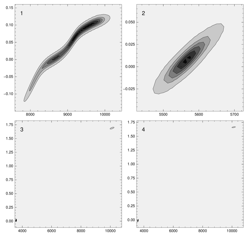
Figure 10: Likelihood contour diagrams for four of the stars in Table 1 using Lejeune atmospheres. From left to right and top to bottom, the cases shown are HD 18331 (A1 V), HD 20794 (G8 V), HD 131976 (M1.5 V), and HD 36395 (M1.5 V). Temperature (in K) is plotted in the horizontal axis and $E(4405-5495)$ in the vertical axis.

• For A-K stars, both runs (with Kurucz and Lejeune atmospheres) produce good results, once the expected uncertainty in the reference temperature for a given spectral type is included. $\mbox{$\chi^{2}_{\rm min}$}/(M-N)$ values are low and a single solution of the correct temperature appears in the likelihood plots (see Fig. 10. The only significant difference between the two atmosphere models for these spectral types takes place for F stars, where the Lejeune atmospheres provide a slightly better fit than the Kurucz ones.

• For B stars, both runs provide essentially identical results but the temperature scale appears to be offset by $\approx 3000$ K for the earliest subtypes. This could be a continuation of the similar effect detected by García & Bianchi (2004) and other authors for O stars using spectroscopic data, as described in the next subsection.

• For M stars. the Kurucz run yields bad fits (large values of $\mbox{$\chi^{2}_{\rm min}$}/(M-N)$) and clearly incorrect temperatures. This indicates that the Kurucz atmospheres do not provide a good representation for some of the optical colors of M dwarfs, as already pointed out by other authors (see, e.g. Lejeune et al. 1998). The Lejeune run yields low values of $\mbox{$\chi^{2}_{\rm min}$}/(M-N)$ (except for HD 209290) and acceptable values of $T$ but with large uncertainties. The explanation for the Lejeune results can be seen in the two lower plots of Fig. 10: two solutions are present, the correct one around 3 650 K and another one around 10  000 K. This implies that the Lejeune atmospheres provide a better representation of the colors of M dwarfs but that $UBVRI$ photometry alone is not enough to distinguish between M stars and reddened late-B stars.

The conclusion is that the addition of $RI$ data to $UBV$ photometry is very useful in constraining the temperature and extinction of stars (under certain assumptions such as knowledge of the extinction law and the luminosity type) and that CHORIZOS can be successfully used to derive those parameters. A possible application of the code would be to automatically generate temperatures and extinctions from photometric surveys such as the one planned with the GAIA mission.

4.2 Measuring optical-IR extinction laws

As a second example, we use Johnson $UBV$ and 2MASS $JHK_{s}$ to determine the extinction and extinction law experienced by an early-type star. We select as input a 35 000 K, $\log g=5.0$, solar metallicity Kurucz atmosphere model with uncertainties of 0.01 magnitudes in each of the six filters. The Kurucz atmosphere is extinguished from $E(4405-5495)$= 0.0 to $E(4405-5495)$= 5.0 using Cardelli et al. (1989) laws from $R_{5495}$= 2.0 to $R_{5495}$= 6.0.

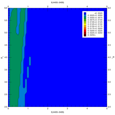
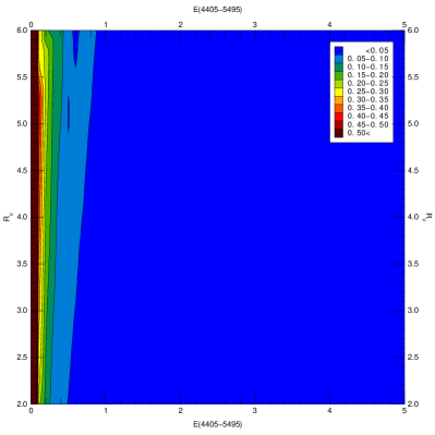
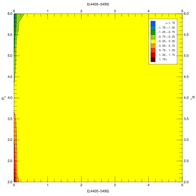
Figure 11: (top) Plots of $\sigma_{E(4405-5495)}$ (left) and $\sigma_{R_{5495}}$ (right) for sample application 2 (main-sequence 35 000 K Kurucz model) as a function of $E(4405-5495)$ and $R_{5495}$ calculated for $UBVJHK$ photometry with uncertainties of 0.01 magnitudes for each filter and restricting the model temperature to its true value. (bottom) Plots of $d_{E(4405-5495)}$ (left) and $d_{R_{5495}}$ (right) corresponding to the same case.

We first assume that we have an accurate spectral type for the star and, therefore, that we know a priori the temperature and gravity of the star. We do this by constraining the temperature and gravity in CHORIZOS to a single value (the true one). Grid extension is used for both $E(4405-5495)$ and $R_{5495}$. Results for this $M=5$, $N=2$ case are shown in Fig. 11. The two lower plots demonstrate that $UBVJHK_{s}$ is an adequate choice of filters to measure the extinction and extinction law experienced by hot stars. The values of both normalized distances are very close to 0.0 everywhere with the only exception of the region around $E(4405-5495)$= 0 for $d_{R_{5495}}$. The latter is an expected behavior, since for low values of the reddening all extinction laws produce similar results and for $E(4405-5495)$= 0.0 they are strictly degenerate. This is evidenced in the upper right plot of Fig. 11: the value of $\sigma_{R_{5495}}$ is kept lower than 0.10 for $\mbox{$E(4405-5495)$}>0.4$ but increases rapidly as we approach $\mbox{$E(4405-5495)$}=0.0$, where the lack of information on the extinction law provided by the data manifests itself in large values of $\sigma_{R_{5495}}$. Note, however, that $\sigma_{E(4405-5495)}$ is not strongly affected by this, since its value is kept below 0.0075 everywhere.

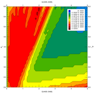
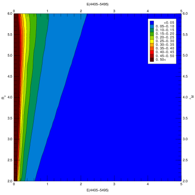
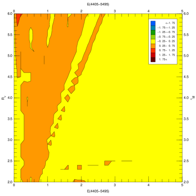
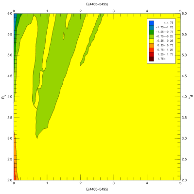
Figure 12: Same as Fig. 11 but without placing constraints on the model temperature.

Suppose now that we know that the star is of early type but we cannot constrain its temperature farther than that due to the lack of an accurate spectral type. We can simulate such a case in CHORIZOS by leaving the temperature unconstrained and selecting main-sequence Kurucz models. Results for this $M=5$, $N=3$ case are shown in Fig. 12. We see in the two lower plots there that the normalized distances are slightly worse than in the previous case, but still within acceptable ranges. The degeneracy in $R_{5495}$ is still present for $E(4405-5495)$= 0.0, as expected, but the information in the photometry is accurate enough to yield good estimates of both $E(4405-5495)$ and $R_{5495}$. The loss of information caused by the unconstrained temperature only translates into larger uncertainties in the measured quantities, but even those are smaller than 0.03 anywhere for $\sigma_{E(4405-5495)}$ and lower than 0.25 for $\sigma_{R_{5495}}$ for $\mbox{$E(4405-5495)$}>0.4$.

Table 2: Comparison between FITMODEL and Cardelli et al. (1989) results for the reddening and extinction law of 4 O stars.

Star	Spectral	Cardelli et al. (1989)		Constrained $T$ and $\log g$ ($M=5$, $N=2$)					Unconstrained $T$ and $\log g$ ($M=5$, $N=4$)
	type	$E(B-V)$	$R_{V}$	$T$ (K)	$\log g$	$E(4405-5495)$	$R_{5495}$	$\frac{\mbox{$\chi^{2}_{\rm min}$}}{M-N}$	$T$ (K)	$\log g$	$E(4405-5495)$	$R_{5495}$	$\frac{\mbox{$\chi^{2}_{\rm min}$}}{M-N}$
HD 46202	O9 V	0.47	3.12	32 500	4.00	0.478$\pm$0.013	3.05$\pm$0.12	1.70	28 900$\pm$1 800	4.13$\pm$0.46	0.448$\pm$0.020	3.14$\pm$0.14	0.57
HD 73882	O8.5 V ((n))	0.72	3.39	32 500	4.00	0.704$\pm$0.017	3.42$\pm$0.10	3.78	28 600$\pm$1 900	4.21$\pm$0.43	0.679$\pm$0.021	3.44$\pm$0.10	5.64
HD 229196	O6 III (n)(f)	1.22	3.12	37 500	3.75	1.221$\pm$0.014	3.16$\pm$0.05	0.47	37 400$\pm$3 400	3.88$\pm$0.56	1.214$\pm$0.028	3.16$\pm$0.06	1.32
CPD $-$59 2600	O6 V ((f))	0.53	4.17	37 500	4.00	0.507$\pm$0.023	4.13$\pm$0.21	1.14	36 500$\pm$3 500	3.90$\pm$0.56	0.492$\pm$0.033	4.14$\pm$0.23	2.17

We also tested the measurement of optical-IR extinction laws with CHORIZOS using real data from the literature. We selected from the sample used by Cardelli et al. (1989) to derive their extinction law the four stars present in the Galactic O star catalog of Maíz-Apellániz et al. (2004) which have (a) $UBVJHK_{s}$ data in the catalog and (b) values of $E(B-V)$ measured by Cardelli et al. (1989) greater than 0.45. CHORIZOS was run using the $UBVJHK_{s}$ photometry ($M=5$) and TLUSTY atmospheres twice, first constraining the temperatures and gravities to fixed values ($N=2$) and then leaving them unconstrained ($N=4$). The values for the temperatures and gravities were derived from the spectral types by using a scale intermediate between the ones proposed by Vacca et al. (1996) and García & Bianchi (2004) and then selecting the closest TLUSTY model. Results are shown in Table 2.

• CHORIZOS results for $R_{5495}$ are in excellent agreement with those of Cardelli et al. (1989). That article does not provide error estimates but our results are always within one sigma and are also small enough for the output to be meaningful.

• CHORIZOS results for $E(4405-5495)$ are also in very good agreement with the reference values, though the unconstrained results are in all cases lower than the ones provided by Cardelli et al. (1989) (but always within two sigmas). The likely origin of this minor difference is the use of values between $-0.30$ and $-0.32$ for the $(B-V)_{0}$ colors of O stars by those authors. TLUSTY atmospheres predict redder colors by $\approx 0.02$ magnitudes. Once that difference is included, the agreement is excellent.

• The $\chi^{2}_{\rm min}$ values indicate very good fits in all cases except for HD 73882, which is still acceptable.

• Assuming that no biases are present (e.g. systematic errors in the TLUSTY atmospheric models), the unconstrained results favor the lower temperature scale of García & Bianchi 2004 (O4 dwarfs around 40  000 K and O6 dwarfs around 32 000-35 000 K, implying a boundary between O and B dwarfs below 30 000 K) over that of Vacca et al. 1996 (with O4 dwarfs close to 50 000 K and a boundary between O and B dwarfs at 34 000 K).

In summary, CHORIZOS can be used to measure reddenings and extinction laws with good precision, even when accurate spectral types are not available.

4.3 What precision is required to measure gravity for O stars with optical photometry alone?

For our third example we want to investigate the possibility of using Strömgren photometry to measure the surface gravity of O stars of unknown temperature and extinction (but with a known extinction law). This is obviously a difficult task, since O-star optical colors are quasi-degenerate in temperature and even more so in gravity. Our goal will be to determine what kind of photometric precision would be required and to assess whether such an accuracy is attainable.

We use TLUSTY atmospheres with solar metallicity, $T=35\,000$ K, and $\log g$ between 3.25 and 4.75 observed with Strömgren $ubvy$ photometry. The extinction law is restricted to be of Cardelli et al. (1989) type with $\mbox{$R_{5495}$}=3.1$ but no constraints are placed on the possible values of $T$, $\log g$, or $E(4405-5495)$, yielding an $M=3$, $N=3$ case. Grid extension is used for $E(4405-5495)$ but not for $T$ or $\log g$ due to the incompleteness of the model grid in these two last parameters (Lanz & Hubeny, 2003).

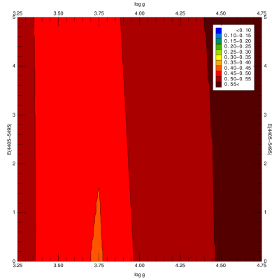
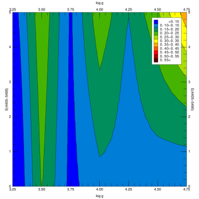
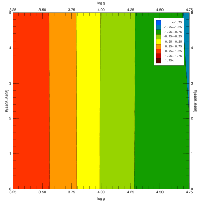
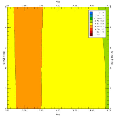
Figure 13: (top) Plots of $\sigma_{\log g}$ for sample application 3 (TLUSTY solar metallicity 35 000 K models) as a function of $\log g$ and $E(4405-5495)$ calculated for Strömgren photometry with uncertainties of 0.003 (left) and 0.001 (right) magnitudes for each filter. (bottom) Plots of $d_{\log g}$ corresponding to the same cases.

In a first run, values of 0.003 were used for the uncertainties in the measured magnitudes. Results for $\sigma_{\log g}$ and $d_{\log g}$ are shown in the left panels of Fig. 13. We see there that the supplied photometry does not yield enough information to measure gravities. The high values of both $d_{\log g}$ and $\sigma_{\log g}$ are characteristic of an almost constant output result of $\approx 4.0\pm 0.5$ for $\log g$ independent of the input values for the gravity and reddening.

In a second run we use values of 0.001 for the uncertainties. Results are shown in the right panels of Fig.13. Now the values for $d_{\log g}$ and $\sigma_{\log g}$ show that some discrimination is possible among gravities, with typical uncertainties in $\log g$ around $0.10-0.20$, which is enough to differentiate between main sequence stars and supergiants.

A hypothetical observer should now ask him/herself: Am I convinced that the atmosphere models are correct to within 0.001 magnitudes? Can I calibrate the photometry to levels good enough to accurately measure differences of 1 milimagnitude? At the current level of knowledge and technology the answers to both questions are likely to be no, hence it can be deduced that at the present time optical photometry alone cannot be used to accurately measure O-star gravities. However, future improvements in atmosphere modeling and photometric accuracies may change the situation.

5 Summary

CHORIZOS is a multi-purpose $\chi^{2}$-minimization SED-fitting code that can be applied to either photometric or spectrophotometric data. In this article we have described the techniques it employs and applied it to several astronomical examples. At the time of this writing, a beta version of the program with a limited number of SED models and 78 filter passbands is available from http://www.stsci.edu/~jmaiz. In the future, a full version will be made available which will include user-defined filter sets or wavelength ranges as well as the possibility of adding other SED models.

Besides the obvious application of selecting the model(s) which are compatible with a given set of observed data, CHORIZOS can be used for a number of other astronomical applications. It can be utilized to select the optimum choice of filters and minimum S/N requires when planning an observation, to test atmospheric models and extinction laws, or to calibrate the zero points of a filter system, to name a few.

 

 

 

 

 

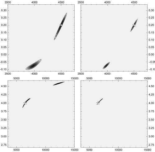
Figure 8: Same as Fig. 7 for two additional cases.

References

- Benítez (2000) Benítez, N. 2000, ApJ, 536, 571
- Bessell et al. (1998) Bessell, M. S., Castelli, F., & Plez, B. 1998, A&A, 333, 231
- Binney & Merrifield (1998) Binney, J., & Merrifield, M. 1998, Galactic Astronomy (Princeton: Princeton University Press)
- Cardelli et al. (1989) Cardelli, J. A., Clayton, G. C., & Mathis, J. S. 1989, ApJ, 345, 245
- Carroll & Ostlie (1996) Carroll, B. W., & Ostlie, D. A. 1996, An introduction to modern astrophysics (Addison-Wesley)
- Cohen et al. (2003) Cohen, M., Wheaton, W. A., & Megeath, S. T. 2003, AJ, 126, 1090
- de Grijs et al. (2003) de Grijs, R., Fritze-v. Alvensleben, U., Anders, P., Gallagher, J. S., Bastian, N., Taylor, V. A., & Windhorst, R. A. 2003, MNRAS, 342, 259
- Fitzpatrick (1999) Fitzpatrick, E. L. 1999, PASP, 111, 63
- García (1989) García, B. 1989, Bulletin d’Information du Centre de Donnees Stellaires, 36, 27
- García & Bianchi (2004) García, M., & Bianchi, L. 2004, ApJ, 606, 497
- Girardi (2000) Girardi, L. 2000, in ASP Conf. Ser. 211, Massive Stellar Clusters, ed. A. Lançon & C. Boily (San Francisco: ASP), 133
- Gordon & Clayton (1998) Gordon, K. D., & Clayton, G. C. 1998, ApJ, 500, 816
- Gould (2003) Gould, A. 2003, astro-ph/0310577
- Koo (1999) Koo, D. C. 1999, in ASP Conf. Ser. 191, Photometric Redshifts and the Detection of High Redshift Galaxies, ed. R. Weymann, L. Storrie-Lombardi, M. Sawicki, & R. Brunner (San Francisco: ASP), 3
- Kurucz (2004) Kurucz, R. L. 2004, http://kurucz.harvard.edu
- Lanz & Hubeny (2003) Lanz, T., & Hubeny, I. 2003, ApJS, 146, 417
- Leitherer et al. (1999) Leitherer, C., Goldader, J. F., González Delgado, R. M., Robert, C., Kune, D. F., de Mello, D. F., Devost, D., & Heckman, T. M. 1999, ApJS, 123, 3
- Lejeune et al. (1997) Lejeune, T., Buser, R., & Cuisinier, F. 1997, A&AS, 125, 229
- Lejeune et al. (1998) Lejeune, T., Cuisinier, F., & Buser, R. 1998, A&AS, 130, 65
- Maíz-Apellániz et al. (2004) Maíz-Apellániz, J., Walborn, N. R., Galué, H. Á., & Wei, L. H. 2004, ApJS, 151, 103
- Mermilliod et al. (1997) Mermilliod, J.-C., Mermilliod, M., & Hauck, B. 1997, A&AS, 124, 349
- Misselt et al. (1999) Misselt, K. A., Clayton, G. C., & Gordon, K. D. 1999, ApJ, 515, 128
- Romaniello et al. (2002) Romaniello, M., Panagia, N., Scuderi, S., & Kirshner, R. P. 2002, AJ, 123, 915
- Vacca et al. (1996) Vacca, W. D., Garmany, C. D., & Shull, J. M. 1996, ApJ, 460, 914
- Whitmore et al. (1999) Whitmore, B. C., Zhang, Q., Leitherer, C., Fall, S. M., Schweizer, F., & Miller, B. W. 1999, AJ, 118, 1551