AcDc - A new code for the NLTE spectral analysis of accretion discs: application to the helium CV AM CVn

We present a recently developed code for detailed NLTE calculations of accretion disc spectra of cataclysmic variables and compact X-ray binaries. Assuming a radial structure of a standard $\alpha$-disc, the disc is divided into concentric rings. For each disc ring the solution of the radiation transfer equation and the structure equations, comprising the hydrostatic and radiative equilibrium, the population of the atomic levels as well as charge and particle conservation, is done self-consistently. Metal-line blanketing and irradiation by the central object are taken into account. As a first application, we show the influence of different disc parameters on the disc spectrum for the helium cataclysmic variable AM CVn.

1 Introduction

Accretion discs are components of objects as diverse as proto-planetary systems, active galactic nuclei, cataclysmic variables or X-ray binaries. A high fraction of the luminosity of these systems may be generated by the accretion disc itself. To understand these objects and interpret the observational data a model of the accretion disc as reliable as possible is necessary. The aim of our work was the development of a program package for the calculation of synthetic spectra and vertical structures of accretion discs considering the physical processes in the disc as accurately as possible.

A fully three-dimensional radiation-hydrodynamic treatment is presently still impossible because of the enormous numerical costs. In the case of a geometrically thin $\alpha$-disc (Shakura & Sunyaev 1973), where the disc thickness is significantly smaller than the disc diameter, the radial and vertical structures can be decoupled. Under the assumption of axial symmetry and by dividing the disc into concentric rings the determination of the vertical structure becomes a one-dimensional problem. The dissipated energy in each disc ring is radiated away at the disc surface, the energy flux can be expressed as effective temperature. As an approximation, it can be assumed that the disc rings are radiating like black bodies. An improvement of the models can be obtained by describing the disc rings by stellar atmosphere models of the same effective temperature, see e.g. Kiplinger (1979), Mayo et al. (1980) or La Dous (1989) in the case of cataclysmic variables and Kolykhalov & Sunyaev (1984) or Sun & Malkan (1989) in the case of AGN. Unfortunately, neither black bodies nor stellar atmosphere models reproduce spectra of accretion discs in an adequate manner (Wade 1988). Meyer & Meyer-Hofmeister (1982), Cannizzo & Wheeler (1984) and Cannizzo & Cameron (1988) calculated the radiative transfer using the diffusion assumption. This assumption is only valid at large optical depths, but the spectrum is generated at optical depths around $\tau\sim 1$, where neither the diffusion assumption nor the assumption of local thermodynamic equilibrium (LTE) is fulfilled. Only solving the radiative transfer equation self-consistently with the structure equations allows the calculation of realistic accretion disc spectra (Kriz & Hubeny 1986, Shaviv & Wehrse 1986, Stoerzer et al. 1994). In the last decade much work in this field was done e.g. by Hubeny & Hubeny (1997, 1998) and Hubeny et al. (2000, 2001).

Following the path mentioned above, we have developed our program package AcDc (Accretion Disc code) for the detailed calculation of vertical structures and NLTE spectra of accretion discs. For each disc ring the equations of radiative and hydrostatic equilibrium as well as the NLTE rate equations for the population numbers of the atomic levels are solved consistently with the radiation transfer equation under the constraint of particle number and charge conservation. Full metal-line blanketing as well as irradiation of the accretion disc by the central object can be considered. By integrating the spectra of the individual disc rings, one obtains a complete disc spectrum for different inclination angles, where the spectral lines are Doppler shifted according to the radial component of the Kepler rotation. This is shown in Sect. 2, whereas in Sect. 3 we show first applications of the developed program package to examine the influence of different parameters on the vertical structure and the spectrum of an accretion disc model for the helium cataclysmic variable AM CVn.

2 Vertical Structure of Accretion Discs

We assume a geometrically thin (disc thickness is significantly smaller than the disc diameter) stationary accretion disc ($\alpha$-disc, Shakura & Sunyaev 1973). We also assume that the mass of the disc is much smaller than the mass of the central object, so we can neglect self-gravitation. Introducing the surface mass density $\Sigma$ as

$$\Sigma\,=\,2\,\int\limits_{0}^{H/2}\rho\,dz\,,$$ (1)

with mass density $\rho$, geometrical height $z$ above the midplane and total disc height $H$, the radial dependence of $\Sigma$ reads following Shakura & Sunyaev (1973)

$$\nu\,\Sigma(R)\,=\,\frac{\dot{M}}{3\pi}\left(1\,-\,\left(\frac{R_{\star}}{R}\right)^{1/2}\right)\,.$$ (2)

Here, $R$ denotes the distance from the central object, $R_{\star}$ the radius of the central object, $\dot{M}$ the mass accretion rate and $\nu$ the kinematic viscosity, defined as

$$\nu\,=\,\alpha\,c_{\rm{s}}\,H\,,$$ (3)

with sound speed $c_{\rm{s}}$ and the parameter $\alpha$ being a measure of the efficiency of angular momentum transport through the disc. The radial distribution of the effective temperature $T_{\rm eff}$ then, following Shakura & Sunyaev (1973), can be described by

$$T_{\rm eff}(R)\,=\,\left[\frac{3GM_{\star}\dot{M}}{8\pi\sigma R^{3}}\left(1\,-\,\left(\frac{R_{\star}}{R}\right)^{1/2}\right)\right]^{1/4}$$ (4)

with $M_{\star}$ denoting the mass of the central object, $G$ the gravitational constant and $\sigma$ the Stefan-Boltzmann constant. The accretion disc is divided into a set of concentric disc rings (cf. Fig. 1). For each ring the vertical structure is calculated by solving the set of equations described in the following two subsections, assuming a plane-parallel geometry.

Figure 1: Geometry of the accretion disc, divided into concentric rings.

2.1 Radiation Transfer Equation

In order to compute the radiation field, which determines the atomic population numbers, the radiation transfer equation has to be solved. This equation describes the modification of the specific intensity $I_{\nu}$ of a ray due to absorption or emission along its path $ds$ through the accretion disc (cf. Fig. 2).

Figure 2: Radiation transfer through the accretion disc layers.

The radiation transfer equation for the shown geometry then reads

$$\mu\,\frac{\partial\,I_{\nu}(\nu,\mu,z)}{\partial\,z}\,=\,-\chi_{\nu}(\nu,z)\,I_{\nu}(\nu,\mu,z)\,+\,\eta_{\nu}(\nu,z)\,.$$ (5)

with the absorption coefficient $\chi_{\nu}$ and the emission coefficient $\eta_{\nu}$. Introducing the source function $S_{\nu}$

$$S_{\nu}\,=\,\frac{\eta_{\nu}}{\chi_{\nu}}\,$$ (6)

the radiation transfer equation is

$$\mu\,\frac{\partial\,I_{\nu}(\nu,\mu,z)}{\partial\,z}\,=\,-\chi_{\nu}(\nu,z)\,(I_{\nu}(\nu,\mu,z)\,-\,S_{\nu}(\nu,\mu,z))\,.$$ (7)

The solution of this equation is a complicated problem, because the source function depends on the radiation field itself. Within an iteration scheme (see below), one solves the radiation transfer equation formally assuming the source function known (cf. Mihalas 1978). In our work this is done by a short characteristics method (Olson & Kunasz 1987). Irradiation of the disc by an external source with a given spectrum is accounted for by an appropriate boundary condition.

2.2 Structure Equations

In order to obtain the atomic population numbers in NLTE all processes populating or de-populating an atomic level are considered. These are ionisation, recombination, excitation and de-excitation, caused either by radiation or collision. Each level $i$ of each ion has one rate equation describing the modification of the population density $n_{i}$ with time $t$:

$$\frac{\partial n_{i}}{\partial t}\,=\,n_{i}\sum_{i\neq j}P_{ij}\,-\,\sum_{j\neq i}n_{j}P_{ji}\,.$$ (8)

$P_{ij}$ denotes the rate coefficients, consisting of radiative and collisional components. Since we assume a hydrostatic stratification, we have

$$\frac{\partial n_{i}}{\partial t}\,=\,0\,.$$ (9)

Assuming that the radial component of the gravitation of the central object equals the centrifugal force of the Keplerian rotation of the disc, the hydrostatic equilibrium of the disc only is determined by the vertical component of the gravitation

$$\frac{dP}{dz}\,=\,-\frac{G\,M_{\star}}{R^{3}}\,z\,\rho\,,$$ (10)

with $P$ denoting the total (gas and radiation) pressure.

Another fundamental equation of the vertical structure describes the local energy balance:

$$E_{\rm{mech}}\,=\,E_{\rm{rad}}\,+\,E_{\rm{conv}}\,.$$ (11)

The viscously generated energy $E_{\rm{mech}}$ is equal to the radiative energy loss $E_{\rm{rad}}$; the convective energy $E_{\rm{conv}}$ term is neglected in the following. For standard $\alpha$-discs, the viscously generated energy reads

$$E_{\rm{mech}}\,=\,\nu\Sigma\left(R\frac{d\omega}{dR}\right)^{2}\,=\,\frac{9}{4}\nu\Sigma\frac{G\,M_{\star}}{R^{3}}$$ (12)

and

$$E_{\rm{rad}}\,=\,4\,\pi\,\int\limits_{0}^{\infty}(\eta(\nu,z)\,-\,\chi(\nu,z)\,J(\nu,z)\,)\,d\nu\,.$$ (13)

Introducing now the mass column depth $m$ as

$$m(z)\,=\,\int\limits_{z}^{\infty}\rho\,dz\,$$ (14)

with the total column mass $M_{0}$ at the midplane the energy dissipated at each depth is

$$E_{\rm{mech}}(m)\,=\,\frac{9}{4}\,\frac{G\,M_{\star}}{R^{3}}\,\nu(m)\,\rho\,.$$ (15)

Here $\nu(m)$ denotes the depth-dependent kinematic viscosity

$$\nu(m)\,=\,a\bar{\nu}(\zeta+1)\left(\frac{m}{M_{0}}\right)^{\zeta}\qquad\mbox{with}\qquad\zeta>0$$ (16)

with the damping factor $\zeta$, which has been introduced by Kriz & Hubeny (1986) to avoid numerical instabilities at the disc surface. $\bar{\nu}$ is the depth-averaged kinematic viscosity with

$$\bar{\nu}\,=\,\frac{1}{M_{0}}\int\limits_{0}^{M_{0}}\nu(m)\,dm\,.$$ (17)

$\bar{\nu}$ corresponds to $\nu$ in Eq. (3) and can be determined by

$$\bar{\nu}\,=\,\frac{Rv_{\phi}}{Re}\,=\,\frac{\sqrt{G\,M_{\star}\,R}}{Re}$$ (18)

with $v_{\phi}$ denoting the Keplerian angular velocity and $Re$ the effective Reynolds number (Lynden-Bell & Pringle 1974). The prescription of the viscosity using the Reynolds number has the advantage that no further assumptions concerning first values of disc height and speed of sound have to be made, as would be necessary using the $\alpha$-prescription. Furthermore, it is possible to describe the depth dependency of the viscosity using the column mass as depth variable. The solution of the energy balance is obtained with a generalised Unsöld-Lucy method (Lucy 1964, Dreizler 2003).

Finally, the total particle density $N$ consists of the sum of the population numbers $n$ of the NLTE and LTE levels $l$ of all ions $i$ of all elements $x$ plus the electron density $n_{\rm{e}}$:

$$N\,=\,\sum_{x=1}^{\rm{element}}\,\sum_{i=1}^{\rm{ion}}\,\left(\sum_{l=1}^{\rm{NLTE}}n_{xil}\,+\,\sum_{l=1}^{\rm{LTE}}n_{xil}^{*}\right)\,+\,n_{\rm{e}}\,.$$ (19)

The equation of charge conservation reads

$$n_{\rm{e}}\,=\,\sum_{x=1}^{\rm{element}}\,\sum_{i=1}^{\rm{ion}}\,q(i)\left(\sum_{l=1}^{\rm{NLTE}}n_{xil}\,+\,\sum_{l=1}^{\rm{LTE}}n_{xil}^{*}\right)\,$$ (20)

with charge $q(i)$ of the ion $i$.

The solution of the system of equations consisting of the radiation transfer equation, the equations of energy balance and hydrostatic equilibrium, the rate equations and the equations of charge and particle conservation is done in an iterative scheme, the so-called Accelerated Lambda Iteration (ALI, Werner & Husfeld 1985; Werner et al. 2003). The input parameters of our models are mass and radius of the central object, radius of the disc ring, mass accretion rate and Reynolds number. Furthermore, the atomic data and an appropriate frequency grid are specified (see e.g. Rauch & Deetjen 2003).

2.3 LTE Start Models

To avoid numerical instabilities at the beginning of the NLTE calculations it is necessary to establish suitable start models under the assumption of LTE. In the following, we summarise the main steps creating such models, according to Hubeny (1990).

To determine the atomic LTE population numbers $n$ the Boltzmann equation

$$\frac{n_{i}}{n_{j}}\,=\,\frac{g_{i}}{g_{j}}\,e^{-(E_{i}-E_{j})/kT}$$ (21)

and the Saha equation

$$\frac{n_{\rm{up}}}{n_{\rm{low}}}\,=\,\frac{2}{n_{\rm{e}}}\left(\frac{2\pi m_{\rm{e}}kT}{h^{2}}\right)^{\frac{3}{2}}\frac{g_{\rm{up}}}{g_{\rm{low}}}e^{-(E_{\rm{up}}-E_{\rm{low}})/kT}$$ (22)

are used instead of the NLTE rate equations. Here, $g$ denotes the statistical weights, $E$ the excitation or ionisation energy, $m_{\rm{e}}$ the electron mass and $h$ the Planck constant. Furthermore, in the case of LTE the source function $S_{\nu}$ equals the Planck function $B_{\nu}$

$$S_{\nu}\,\equiv\,B_{\nu}\,.$$ (23)

To get an analytical expression for the vertical temperature structure one combines the first momentum of the specific intensity and the equation of the energy balance. Then the equation for the vertical temperature structure in the case of LTE finally reads

$$T^{4}\,=\,\frac{3}{4}T_{\rm eff}^{4}\left(\tau_{\rm{R}}\left(1-\frac{\tau_{\rm{R}}}{2\tau_{\rm{tot}}}\right)+\frac{1}{\sqrt{3}}+\frac{1}{3\epsilon\tau_{\rm{tot}}}\frac{w}{\bar{w}}\right)\,$$ (24)

with $\epsilon\,=\,\kappa_{\rm{B}}M_{0}/\tau_{\rm{tot}}$ and

$$\kappa_{\rm{B}}\,\,=\,\frac{1}{B}\int\limits_{0}^{\infty}(\kappa_{\nu}/\rho)\,B_{\nu}\,d\nu\,.$$ (25)

The equation of the hydrostatic equilibrium has the same form as in the case of NLTE, but can alternatively be transformed into a differential equation of second order:

$$\frac{d^{2}P}{dm^{2}}\,=\,-\frac{c_{\rm{s}}^{2}}{P}\frac{G\,M_{\star}}{R^{3}}\,.$$ (26)

The solution of this equation is done numerically. The upper boundary condition reads, following Hubeny (1990),

$$P(1)\,=\,\frac{m_{1}c_{\rm{s}}^{2}}{H_{\rm{g}}}\frac{1}{f(\frac{z-H_{\rm{r}}}{H_{\rm{g}}})}$$ (27)

with

$$f(x)\,=\,\frac{\sqrt{\pi}}{2}e^{x^{2}}\,k(x)$$ (28)

and

$$k(x)\,=\,\frac{2}{\sqrt{\pi}}\int\limits_{x}^{\infty}e^{-t^{2}}dt\,.$$ (29)

Here, $H_{\rm{g}}$ and $H_{\rm{r}}$ denote the gas and radiation pressure scale height, defined as

$$H_{\rm{g}}\, = \,\sqrt{\frac{2c_{\rm{g}}^{2}}{GM_{\star}/R^{3}}}\,,$$ (30)

$$H_{\rm{r}}\, = \,\frac{\sigma}{c}T_{\rm eff}^{4}\kappa_{H}\frac{GM_{\star}}{R^{3}}$$ (31)

with $c_{g}$ denoting the sound speed associated with gas pressure

$$c_{\rm{g}}^{2}\,=\,\frac{P_{\rm{g}}}{\rho}\,.$$ (32)

2.4 The Synthetic Spectrum

Having now calculated the vertical structures and spectra of the individual disc rings, the ring spectra are integrated to get the spectrum of the whole accretion disc:

$$I(\nu,i)\,=\,\cos(i)\int\limits_{R_{\rm{i}}}^{R_{\rm{o}}}\int\limits_{0}^{2\pi}I(\nu,i,\phi,r)\,r\,d\phi\,dr\,.$$ (33)

Here, $R_{\rm{i}}$ and $R_{\rm{o}}$ denote the inner and outer radius of the disc, $i$ is the inclination angle (cf. Fig. 3). The integration over the azimuthal angle $\phi$ is done in intervals of $1^{\circ}$.

Figure 3: Accretion disc geometry.

In this last step, spectral lines become broadened due to the Keplerian rotation of the disc.

3 Synthetic Spectrum for AM CVn

In order to test and gain experience with AcDc our first application was the calculation of the synthetic spectrum of AM CVn for a comparison with results of a recent analysis performed by Nasser et al. (2001).

3.1 AM CVn

AM CVn is the prototype of the so-called AM CVn stars or helium cataclysmics, a subgroup of the cataclysmic variables. They are thought to be the end product of the evolution of close binary systems (El-Khoury & Wickramasinghe, 2000). The first observations of AM CVn have been made by Malmquist (1936) and Humason & Zwicky (1947). Greenstein & Matthews (1957) classified AM CVn as a helium-rich white dwarf, Burbidge et al. (1967) as a quasi-stellar object, and Wambler (1967) as a hot star. After the discovery of periodic variability in the light curve (Smak 1967), Warner & Robinson (1972) proposed AM CVn to be a close binary system with ongoing mass transfer. Right now, these systems are believed to be interacting white dwarf binary systems, consisting of a degenerate C/O white dwarf as primary and a semi-degenerate low-mass secondary, composed of almost pure helium. The secondary fills its Roche volume and loses mass via Roche-Lobe overflow onto the primary, generating an accretion disc around it.

AM CVn itself has been analysed by Nasser et al. (2001) using TLUSDISC (Hubeny 1990). They showed that the system consists of a primary of about 1.1 $\rm M_{\odot}$ and a secondary of about 0.09 $\rm M_{\odot}$. The radius of the primary is 4600 km, and the mass accretion rate is about $3\cdot 10^{-9}\,\rm M_{\odot}/yr$. For the calculations, we assumed an inner radius of 1.4 $\rm{R_{\star}}$ and an outer radius of 15 $\rm{R_{\star}}$, both values were varied to explore the influence of the disc size onto the spectrum. The Reynolds number was set to 15 000, the damping factor $\zeta$ was chosen to be 0.001. Convective energy transport is not yet included in AcDc, so we had to neglect convection, fortunately without getting numerical problems in the outer part of the disc. The number ratio H/He was set to $10^{-5}$, and abundances of carbon, nitrogen, oxygen, and silicon were assumed to be solar. The self-consistent inclusion of metals is an improvement over the Nasser et al. (2001) models. Some details concerning the ions, levels and lines we used in our calculations are shown in Table 1. The atomic data are taken from the opacity project (Seaton et al. 1994) and the Kurucz line lists (1991). The Lyman, Balmer and Paschen series of H i, the Lyman series of Hei and the Lyman, Balmer, Paschen and Bracket series of Heii, some Lyman and Balmer lines of metals as well as resonance lines are Stark broadened, all other line profiles are Doppler broadened. For the line broadening of H we use VCS tables (Lemke 1997), for the line broadening of He i we use BCS tables (Barnard, Cooper & Shamey 1969) and Griem tables (Griem 1974), for He ii we use VCS tables (Schöning & Butler 1989). In total, we calculated 38 individual disc rings.

Table 1: Some details concerning the ions and the number of NLTE levels and lines used in our calculations.

Ion	NLTE levels	lines	Ion	NLTE levels	lines
H i	16	29	N ii	2	0
H ii	1	-	N iii	34	67
He i	44	31	N iv	34	53
He ii	32	59	N v	36	56
He iii	1	-	N vi	1	0
C ii	16	25	O ii	26	36
C iii	58	124	O iii	28	37
C iv	36	86	O iv	11	5
C v	1	0	O v	6	1
			O vi	36	48
			O vii	1	0

3.2 Influence of Disc Parameters on the Spectrum

First, we examined the influence of different inner and outer radii onto the spectrum of the disc. We varied the inner radius from 1.4 to 2 $\rm R_{\star}$ and the outer radius from 11 to 15 $\rm R_{\star}$.

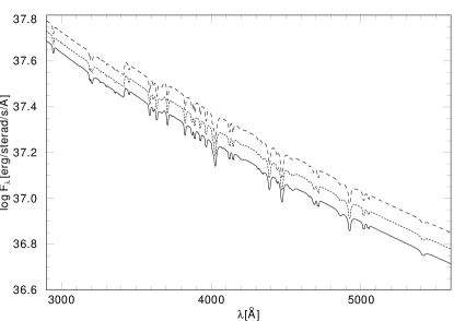
Figure 4: Optical spectra of three accretion disc models with outer radii of 11 $\rm R_{\star}$ (solid line), 13 $\rm R_{\star}$ (dotted) and 15 $\rm R_{\star}$ (dashed). The mass accretion rate is $3\cdot 10^{-9}\,\rm M_{\odot}/yr$ and the inclination is $10^{\circ}$.

Figure 5: Detail of Fig. 4 with three accretion disc models with outer radii of 11 $\rm R_{\star}$ (solid line), 13 $\rm R_{\star}$ (dotted) and 15 $\rm R_{\star}$ (dashed).

Figure 4 shows the optical spectrum of three disc models with outer radii of 11 $\rm R_{\star}$, 13 $\rm R_{\star}$ and 15 $\rm R_{\star}$. The mass accretion rate is $3\cdot 10^{-9}\,\rm M_{\odot}/yr$, the inclination is $10^{\circ}$. One can clearly see the increasing total flux with increasing outer radius because of the increasing radiating surface. Figure 5 shows details of the normalised spectrum. The line cores of He i become deeper with increasing outer radius because the large outer regions of the disc are cool enough to show strong He i lines. Variation of the inner radius shows similar, but smaller effects on the lines.

Second, we analysed the influence of different inclination angles on the spectrum.

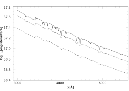
Figure 6: Optical spectra of an accretion disc model seen under three different inclination angles, 10^∘ (solid line), 36^∘ (dotted) and 60^∘ (dashed). The inner radius of the disc is 1.4 $\rm R_{\star}$, the outer radius 15 $\rm R_{\star}$ and the mass accretion rate is $3\cdot 10^{-9}\,\rm M_{\odot}/yr$.

Figure 7: Detail of Fig. 6 with an accretion disc model seen under three different inclination angles, 10^∘ (solid line), 36^∘ (dotted) and 60^∘ (dashed).

Figure 6 shows a disc model seen under three different inclination angles. The total flux decreases with increasing inclination angle because of the decreasing projected surface. As shown in Fig. 7, narrow lines at small inclination angles become broad lines at high inclination angles because of the increasing rotational broadening.

3.3 Vertical Structure

Figure 8: Vertical distribution of temperature, density and Rosseland optical depth of three representative disc rings with radii of 1.4 $\rm R_{\star}$ (solid line), 7 $\rm R_{\star}$ (dotted line) and 15 $\rm R_{\star}$ (dashed line).

In Fig. 8 the vertical distribution of temperature, density and Rosseland optical depth of three representative disc rings at 1.4 $\rm R_{\star}$, 7 $\rm R_{\star}$ and 15 $\rm R_{\star}$ is shown. According to Eq. (4) disc rings from the outer part of the disc are cooler than inner disc rings. The temperature decreases monotonously from the midplane to the surface of the rings. Disc rings composed only of H and He, but without C, N, and O show an increase of the temperature in the outer layers near the surface.

3.4 Model vs. Observation

Finally we compared our accretion disc model spectra with an observed spectrum of AM CVn, obtained at the 6 m BAT of the SAO in May 2002.

Figure 9 shows the observed spectrum and three model spectra with outer radii of 11 $\rm R_{\star}$, 13 $\rm R_{\star}$ and 15 $\rm R_{\star}$, respectively. The inner radius is 1.4 $\rm R_{\star}$, the inclination is 36^∘ and the mass accretion rate is $3\cdot 10^{-9}\,\rm M_{\odot}/yr$. Owing to the larger and at the same time cooler radiating surface, a larger outer radius leads to an increase of the spectral line strengths of neutral helium compared to those of ionized helium.

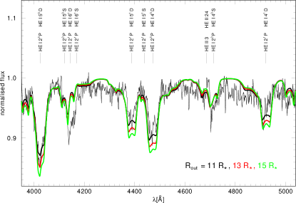
Figure 9: Comparison of the observed spectrum (thin line) with model spectra of the AM CVn disc for 3 different outer radii.

Figure 10 shows the influence of the inclination angle on the spectrum. The disc models with inclination angles of 23^∘, 48^∘ and 70^∘ extend from 1.4 $\rm R_{\star}$ to 13 $\rm R_{\star}$ and the mass accretion rate is $3\cdot 10^{-9}\,\rm M_{\odot}/yr$. The larger the inclination angle, the stronger the spectral lines are broadened due to the increasing radial component of the Kepler velocity.

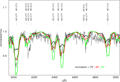
Figure 10: Comparison of the observed spectrum (thin line) with model spectra of the AM CVn disc for 3 different inclination angles.

In Fig. 11 our best fit is shown. The disc model extends from 1.4 $\rm R_{\star}$ to 13 $\rm R_{\star}$, the inclination is 36^∘ and the mass accretion rate is $3\cdot 10^{-9}\,\rm M_{\odot}/yr$. The shapes of the He i lines are in good agreement with the observation.

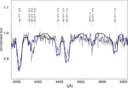
Figure 11: Comparison of the observed spectrum (thin line) with a model spectrum of the AM CVn disc.

4 Conclusions

1. We developed the new code AcDc for detailed NLTE calculations of accretion disc spectra of cataclysmic variables and compact X-ray binaries, solving the radiation transfer equation self-consistently together with the structure equations under consideration of full metal line blanketing as well as irradiation of the accretion disc by the central object.

2. Variation of the extension of the disc has a significant influence on the spectrum of the AM CVn disc. Lines of He i become deeper with increasing outer radius. In addition, the inclination angle of the disc has a clear influence on the spectral lines by Kepler rotation.

3. The comparison of model spectra with an observed spectrum of AM CVn yields 1.4 $\rm R_{\star}$ for the inner radius and 13 $\rm R_{\star}$ for the outer radius, the inclination is found to be 36^∘ and the mass accretion rate $3\cdot 10^{-9}\,\rm M_{\odot}/yr$. This is in agreement with results of Nasser et al. (2001).

For future work, we plan to include further physical processes in the program, e.g. Comptonisation as well as convective energy transport, into the program. Furthermore, we have started to study winds from the accretion disc. A depth dependent atomic model will be employed to overcome numerical instabilities in irradiated discs due to extremely weak populated atomic levels at some depths.

- (1) Barnard, A.J., Cooper, J., & Shamey, L.J. 1969, A&A, 1, 28
- (2) Burbidge, G., Burbidge, M., & Hoyle, F. 1967, ApJ, 147, 1219
- (3) Cannizzo, J.K., & Wheeler, J.C. 1984, ApJS, 55, 367
- (4) Cannizzo, J.K., & Cameron, A.G.W. 1988, ApJ, 330, 327
- (5) Dreizler, S. 2003, in Stellar Atmosphere Modelling, ed. I. Hubeny, D. Mihalas, and K. Werner, ASP Conference Proceedings, 288, 69
- (6) El-Khoury, W., & Wickramasinghe, D. 2000, A&A, 358, 154
- (7) Greenstein, J.L., & Matthews, M.S. 1957, ApJ, 126, 14
- (8) Griem, H.R. 1974, Spectral line broadening by plasmas, Pure and Applied Physics, New York, Academic Press, 1974
- (9) Hubeny, I. 1990, ApJ, 351, 632
- (10) Hubeny, I., & Hubeny, V. 1997, ApJ, 484, L37
- (11) Hubeny, I., & Hubeny, V. 1998, ApJ, 505, 558
- (12) Hubeny, I., Agol, E., Blaes, O., & Krolik, J.H. 2000, ApJ, 533, 710
- (13) Hubeny, I., Blaes, O., Krolik, J.H., & Agol, E. 2001, ApJ, 559, 680
- (14) Humason, M.L., & Zwicky, F. 1947, ApJ, 105, 85
- (15) Kiplinger, A.L. 1979, ApJ, 234, 997
- (16) Kolykhalov, P.I., & Sunyaev, R.A. 1984, Advances in Space Research, 3, 249
- (17) Kriz, S., & Hubeny, I. 1986, Bulletin of the Astronomical Institutes of Czechoslovakia, 37, 129
- (18) Kurucz, R. 1991, NATO ASI Series C, 341, 441
- (19) La Dous, C. 1989, A&A, 211, 131
- (20) Lemke, M. 1997, A&AS, 122, 285
- (21) Lucy, L.B. 1964, in 1st Harvard-Smithsonian Conference on Stellar Atmospheres, SAO Special Report No. 167, 93
- (22) Lynden-Bell, D., & Pringle, J.E. 1974, MNRAS, 168, 603
- (23) Malmquist, K.G. 1936, in Stockholms Observatoriums Annaler Vol. 12, 7, 130
- (24) Mayo, S.K., Wickramasinghe, D.T., & Whelan, J.A.J. 1980, MNRAS, 193, 793
- (25) Meyer, F., & Meyer-Hofmeister, E. 1982, A&A, 106, 34
- (26) Mihalas, D. 1978, Stellar Atmospheres, San Francisco, W. H. Freeman and Co.
- (27) Nasser, M.R., Solheim, J.-E., & Semionoff, D.A. 2001, A&A, 373, 222
- (28) Olson, G.L., & Kunasz, P.B. 1987, JQSRT, 38, 325
- (29) Rauch, T., & Deetjen, J.L. 2003, in Stellar Atmosphere Modeling, ed. I. Hubeny, D. Mihalas, and K. Werner, ASP Conference Proceedings, 288, 103
- (30) Schöning, T., & Butler, K. 1989, A&AS, 78, 51
- (31) Seaton, M., Yan, Y., Mihalas, D., & Pradhan, A. 1994, MNRAS, 266, 805
- (32) Shakura, N.I., & Sunyaev, R.A. 1973, A&A, 24, 337
- (33) Shaviv, G., & Wehrse, R. 1986, A&A, 159, L5
- (34) Smak, J. 1967, Acta Astronomica, 17, 255
- (35) Stoerzer, H., Hauschildt, P.H., & Allard, F. 1994, ApJL, 437, L91
- (36) Sun, W., & Malkan, M.A. 1989, ApJ, 346, 68
- (37) Wade, R.A. 1988, ApJ, 335, 394
- (38) Wampler, E.J. 1967, ApJL, 149, L101
- (39) Warner, B., & Robinson, E.L. 1972, MNRAS, 159, 101
- (40) Werner, K., & Husfeld, D. 1985, A&A, 148, 417
- (41) Werner, K., Deetjen, J.L., Dreizler, S., Nagel, T., Rauch, T., & Schuh, S. L. 2003, in Stellar Atmosphere Modeling, ed. I. Hubeny, D. Mihalas, and K. Werner, ASP Conference Proceedings, 288, 31