Correlation Function in Deep Redshift Space as a Cosmological Probe

Abstract

Recent development of galaxy surveys enables us to investigate the deep universe of high redshift. We quantitatively present the physical information extractable from the observable correlation function in deep redshift space in a framework of the linear theory. The correlation function depends on the underlying power spectrum, velocity distortions, and the Alcock-Paczyński (AP) effect. The underlying power spectrum is sensitive to the constituents of matters in the universe, the velocity distortions are sensitive to the galaxy bias as well as the amount of total matter, and the Alcock-Paczyński effect is sensitive to the dark energy components. Measuring the dark energy by means of the baryonic feature in the correlation function is one of the most interesting applications. We show that the “baryon ridge” in the correlation function serves as a statistically circular object in the AP effect. In order to sufficiently constrain the dark energy components, the redshift range of the galaxy survey should be as broad as possible. The survey area on the sky should be smaller at deep redshifts than at shallow redshifts to keep the number density as dense as possible. We illustrate an optimal survey design that are useful in cosmology. Assuming future redshift surveys of $z\lower 2.15277pt\hbox{$\;\buildrel<\over{\sim}\;$}3$ which are within reach of the present-day technology, achievable error bounds on cosmological parameters are estimated by calculating the Fisher matrix. According to an illustrated design, the equation of state of dark energy can be constrained within $\pm 5\%$ error assuming that the bias is unknown and marginalized over. Even when all the other cosmological parameters should be simultaneously determined, the error bound for the equation of state is up to $\pm 10\%$.

1. Introduction

Observing galaxy clustering in deep redshift surveys is one of the most direct way to probe the evolution and structure of our universe itself. Recent advances in observational technologies of deep surveys are spectacular, and enormous amount of information on deep universe must be flooded in near future. To understand the cosmological meaning of galaxy clustering in deep universe, theoretical analysis of the clustering of observed galaxies are necessary.

The observable objects in the deep redshift surveys are fainter than the shallow surveys, and the sampling number density per comoving volume is smaller if we adopt selection criteria by apparent magnitude of galaxies. When one is interested in linear clustering regime, where complex nonlinear dynamics is not relevant, the mean separation of the objects should be at least of order $10{\hbox{$\,h^{-1}$}{\rm Mpc}}$. Recent advances of redshift surveys, such as the Deep Extragalactic Evolutionary Probe survey (DEEP; Davis et al., 2003), and the Sloan Digital Sky Survey (SDSS; York et al., 2000), etc. can map such fainter objects with sufficient qualities. By an efficient color-selection technique, the sampling number density can be improved.

The deep redshift surveys, if the sampling density is large enough, have many advantages. First, the observable volume at deep redshifts is much larger than that at shallow redshifts, simply because the available volume is large in distant space. Second, the nonlinear clustering properties are less important at a fixed scale in deep surveys, because the universe is younger in deep universe and there is less time for the density fields to evolve nonlinearities. Third, while the observations of the nearby universe can map only the snapshot of the recent universe, the observations of the deep universe reveal the evolutionary properties of the universe. This is an indispensable information to establish a consistent picture of the whole universe.

The measurements of the cosmic microwave background, such as the Wilkinson Microwave Anisotropy Probe (WMAP) satellite (Bennett et al., 2003), provide the information of the universe at very high redshift, $z\simeq 1100$. On the other hand, the traditional galaxy redshift surveys, such as the Las Campanas Redshift Survey (LCRS, Shectman et al., 1996), IRAS Point Source Catalog Redshift Survey (PSCz, Saunders et al., 2000), and the AAT two-degree field galaxy redshift survey (2dFGRS, Colless et al., 2001) reveal the recent universe, $z\lower 2.15277pt\hbox{$\;\buildrel<\over{\sim}\;$}0.2$. Systematic investigations of the universe between these redshifts are undoubtedly promising ways to unveil the evolutionary feature of the universe. Especially, the galaxy redshift surveys of redshift range of $z=0.2$–$3.0$ can be attainable by present-day technology. The Kilo-Aperture Optical Spectrograph (KAOS) project is proposed to survey galaxies at those redshifts with sufficient density, using one of the existing Gemini telescopes.

One of the most significant feature of the universe one can probe by such deep redshift surveys is the nature of the dark energy component of the universe. The dark energy component does not have important contributions at very high redshifts. The effects of the dark energy can be probed by studying how the recent universe evolves with redshifts. One of the striking evidence of the dark energy was provided by the luminosity distance–redshift relation of type Ia supernovae (Riess et al., 1998; Perlmutter et al., 1999) at redshifts $z\lower 2.15277pt\hbox{$\;\buildrel<\over{\sim}\;$}1$. The galaxy redshift surveys had not been considered to provide constraints on the dark energy, since the galaxy surveys had been restricted to the low-redshift universe at $z\lower 2.15277pt\hbox{$\;\buildrel<\over{\sim}\;$}0.2$. The ongoing and future galaxy surveys will break this limitation and the evolutionary features of the universe, including dark energy properties, will be searched by galaxy surveys. A machinery of probing the dark energy by galaxy surveys is based on the extended Alcock-Paczyński (AP) effects (Alcock & Paczyński, 1979; Ballinger, Peacock & Heavens, 1996; Matsubara & Suto, 1996) on galaxy clustering in redshift space. Recently, several authors investigate the feasibility of detecting the nature of the dark energy from the extended AP effects of the correlation function (Matsubara & Szalay, 2003) and the power spectrum (Blake & Glazebrook, 2003; Seo & Eisenstein, 2003; Hu & Haiman, 2003; Linder, 2003).

Theoretical predictions of the extended AP effect are easier when the power spectrum is used, because the dependences of the observed power spectrum with AP effect on cosmological parameters are not complicated once the dependence on the mass power spectrum is known. Including simultaneously the peculiar velocity effect (Kaiser, 1987) and the AP effect on the power spectrum requires only simple procedures to implement (Ballinger, Peacock & Heavens, 1996). However, observational determination of the reliable power spectrum requires a homogeneous sample, since the observed spectrum is a convolution of the survey geometry and the real density spectrum. On the other hand, the correlation function is more straightforward to observationally determine. Once the selection function of the survey is known, the correlation function is obtained by simple pair countings even when the survey selection is inhomogeneous and the geometrical shape of the survey is complex. Although the theoretical calculation of the two-point correlation function in redshift space is not as obvious as that of the power spectrum, we now have an analytical formula which make a numerical implementation very fast (Matsubara, 2000; Matsubara, Szalay, & Pope, 2004). The last formula also contains wide-angle effects of the survey, which can not be naturally implemented in the power spectrum analysis.

The purpose of this paper is to provide a thorough analysis of the two-point correlation function in deep redshift space and its dependence on cosmological parameters. The cosmological information contained in the correlation function is quantitatively investigated. As a result, we provide error forecasts of the cosmological parameters probed by the correlation function in a given redshift survey. Complementarity of samples at different redshifts is quantitatively addressed. The analysis in this paper provides useful information for the design of the future surveys at deep redshifts.

This paper is organized as follows. In §2, a compact version of the analytic expression of the correlation function in arbitrarily deep redshift space, derived from a more general expression of the previous work is presented. Physical contents in the analytic formula are addressed in §3. In §4, series of deep redshift surveys which are within reach of the present-day technology are considered and expected error bounds are estimated by means of the Fisher information matrix. Optimal designs for the future redshift surveys are indicated. Conclusions and discussion are given in §5. Some basic notations are introduced in Appendix A. Useful equations in calculating the Fisher matrix with marginalizations are given in Appendix B.

2. The Analytic Expression of the Correlation Function in Deep Redshift-space

We analyze the structure of the two-point correlation function in deep redshift space, using the analytic formula derived in the most general situation by relativistic linear perturbation theory (Matsubara, 2000). In this section, the result of the analytic formula is briefly reviewed. Some basic notations of the Friedmann-Lemaître model with dark energy extension are introduced in Appendix A.

The general two-point correlation function in redshift space is a function of the redshifts $z_{1}$, $z_{2}$ of the two points, and the angle $\theta$ between them. The analytic result of Matsubara (2000) has the form,

$$\xi(z_{1},z_{2},\theta)=D(z_{1})D(z_{2})\left[b(z_{1})b(z_{2})\xi^{(0)}(z_{1},z_{2},\theta)\right.$$

$$\quad+\,f(z_{1})b(z_{2})\xi^{(1)}(z_{1},z_{2},\theta)+f(z_{2})b(z_{1})\xi^{(1)}(z_{2},z_{1},\theta)$$

$$\quad\left.+\,f(z_{1})f(z_{2})\xi^{(2)}(z_{1},z_{2},\theta)\right],$$ (1)

where $b(z)$ is the redshift-dependent linear bias factor and $D(z)$ is the linear growth factor normalized as $D(z=0)=1$, and calculated by the differential equations (A5) and (A6). The functions $\xi^{(n)}$ are defined below. In this paper, we assume the concerning scales of the two-point correlation function are reasonably smaller than the curvature scale of the universe: $x_{12}\ll|K|^{-1/2}$, where $x_{12}$ is the comoving distance between the two points. This exactly holds for a flat universe, and is fulfilled in practice because the curvature of the universe is observationally at least 20 times larger than the Hubble scale, $c/H_{0}$, since ${\mit\Omega}_{K0}={\mit\Omega}_{M0}+{\mit\Omega}_{{\mit\Lambda}0}-1=0.02\pm 0.02$ (Spergel et al., 2003). This approximation does not necessarily require that the comoving distances to the two points from the observer, $x(z_{1})$ and $x(z_{2})$, are smaller than the curvature scale. In fact, the curvature effects are included in those distances in the following compact version of the formula.

Adopting the above approximation, the components $\xi^{(k)}$ in the analytic formula (1) are given by

$$\xi^{(0)}(z_{1},z_{2},\theta)=\xi^{(0)}_{0}(x_{12}),$$ (2)

$$\xi^{(1)}(z_{1},z_{2},\theta)=\frac{1}{3}\xi^{(0)}_{0}(x_{12})+A_{12}\cos\gamma_{12}\xi^{(1)}_{1}(x_{12})$$

$$\qquad\qquad\qquad\quad+\,\left(\cos^{2}\gamma_{12}-\frac{1}{3}\right)\xi^{(1)}_{2}(x_{12}),$$ (3)

$$\xi^{(2)}(z_{1},z_{2},\theta)=\frac{1}{15}\left(1+2\cos^{2}\theta\right)\xi^{(0)}_{0}(x_{12})$$

$$\qquad-\,\frac{1}{3}A_{12}A_{21}\cos\theta\xi^{(1)}_{0}(x_{12})$$

$$\qquad+\,\frac{1}{5}\left[A_{12}\left(\cos\gamma_{12}-2\cos\gamma_{21}\cos\theta\right)\right.$$

$$\qquad\qquad\left.+\,A_{21}\left(\cos\gamma_{21}-2\cos\gamma_{12}\cos\theta\right)\right]\xi^{(1)}_{1}(x_{12})$$

$$\qquad-\,\frac{1}{7}\biggl{[}\frac{2}{3}+\frac{4}{3}\cos^{2}\theta-\left(\cos^{2}\gamma_{12}+\cos^{2}\gamma_{21}\right)$$

$$\qquad\qquad\qquad+\,4\cos\gamma_{12}\cos\gamma_{21}\cos\theta\biggr{]}\xi^{(1)}_{2}(x_{12})$$

$$\qquad+\,A_{12}A_{21}\left(\cos\gamma_{12}\cos\gamma_{21}+\frac{1}{3}\cos\theta\right)\xi^{(2)}_{2}(x_{12})$$

$$\qquad+\,\frac{1}{5}\left[A_{12}\left(5\cos\gamma_{12}\cos^{2}\gamma_{21}-\cos\gamma_{12}+2\cos\gamma_{21}\cos\theta\right)\right.$$

$$\qquad\quad\left.+\,A_{21}\left(5\cos\gamma_{21}\cos^{2}\gamma_{12}-\cos\gamma_{21}+2\cos\gamma_{12}\cos\theta\right)\right]$$

$$\qquad\qquad\qquad\qquad\qquad\times\,\xi^{(2)}_{3}(x_{12})$$

$$\qquad+\,\frac{1}{7}\biggl{[}\frac{1}{5}+\frac{2}{5}\cos^{2}\theta-\left(\cos^{2}\gamma_{12}+\cos^{2}\gamma_{21}\right)$$

$$\qquad\qquad\qquad+\,4\cos\gamma_{12}\cos\gamma_{21}\cos\theta$$

$$\qquad\qquad\qquad+\,7\cos^{2}\gamma_{12}\cos^{2}\gamma_{21}\biggr{]}\xi^{(2)}_{4}(x_{12}).$$ (4)

In the above equations, the functions $\xi^{(n)}_{l}$ are defined by

$$\xi^{(n)}_{l}(x)=\frac{(-1)^{n+l}}{x^{2n-l}}\int\frac{k^{2}dk}{2\pi^{2}}\frac{j_{l}(kx)}{k^{2n-l}}P(k),$$ (5)

where $j_{l}$ is the spherical Bessel function, and $x_{12}$ denotes the comoving distance between two points specified by variables $(z_{1},z_{2},\theta)$. An explicit representation of $x_{12}$ is given by

$${x_{12}} \simeq {S_{K}}(x_{12})$$ (6)

$$= \left[{S}^{2}(z_{1})+{S}^{2}(z_{2})-2C(z_{1})C(z_{2})S(z_{1})S(z_{2})\cos\theta\right.$$

$$\qquad\qquad\left.-\,K{S}^{2}(z_{1}){S}^{2}(z_{2})\left(1+\cos^{2}\theta\right)\right]^{1/2},$$

where the first approximation is consisitent with $x_{12}\ll|K|^{-1/2}$, and

$$S(z) \equiv S_{K}[x(z)]$$ (10)

$$= \left\{\begin{array}[]{ll}(-K)^{-1/2}{\rm sinh}\left[(-K)^{1/2}x(z)\right],&(K<0),\\ x(z),&(K=0),\\ K^{-1/2}\sin\left[K^{1/2}x(z)\right],&(K>0),\end{array}\right.$$

$$C(z) \equiv \frac{dS_{K}}{dx}(z)=\left\{\begin{array}[]{ll}\cosh\left[(-K)^{1/2}x(z)\right],&(K<0),\\ 1,&(K=0),\\ \cos\left[K^{1/2}x(z)\right],&(K>0).\end{array}\right.$$ (14)

The angle $\gamma_{12}$ is the angle between the separation $x_{12}$ and the line of sight at the first point of $z_{1}$, and $\gamma_{21}$ is the similar angle at the second point of $z_{2}$. Trigonometric geometry shows that they are analytically represented by

$$\cos\gamma_{12}=\frac{S(z_{1})C(z_{2})-C(z_{1})S(z_{2})\cos\theta}{S_{K}(x_{12})},$$ (15)

and $\cos\gamma_{21}$ is given by a replacement of $z_{1}\leftrightarrow z_{2}$ in the above equation. If the universe is exactly flat, the above equation simply reduces to $\cos\gamma_{12}=(x_{1}-x_{2}\cos\theta)/x_{12}$. In this paper, we generally consider a non-flat universe as well as a flat universe. The quantities $A_{12}$ and $A_{21}$ are needed when the redshift evolution of the clustering between the two points and that of the selection function is not negligible, and are given by

$$A_{12}=S_{K}(x_{12})H(z_{1})\frac{d}{dz_{1}}\ln[H(z_{1})D(z_{1})f(z_{1})n(z_{1})],$$ (16)

and the corresponding equation of $A_{21}$ with a replacement $z_{1}\leftrightarrow z_{2}$ in this equation. In the above equation, $n(z)=dN(<z)/dz$ is the selection function including the volume factor, i.e., the differential number count of galaxies within a fixed angular area as a function of redshift $z$. Since $H(z)d/dz=d/dx$, the quantities $A_{12}$ and $A_{21}$ have the order of relative difference of the product $H(z)D(z)f(z)n(z)$ between $z_{1}$ and $z_{2}$. Therefore, if the difference of this product is negligible between two points at $z_{1}$ and $z_{2}$, the terms with quantities $A_{12}$ and $A_{21}$ can be omitted. Since the characteristic scales on which the factors $H(z)$, $D(z)$, and $f(z)$ vary are of order of the Hubble scale, it is unlikely that the contributions of these factors are important. In practice, the determination of the galaxy correlation function on Hubble scales is extremely difficult because of the high signal-to-noise ratio. A possible dominant contribution to $A_{12}$ and $A_{21}$ is from the selection function $n(z)$, and therefore, $A_{12}=S_{K}(x_{12})H(z_{1})d\ln[n(z_{1})]/dz_{1}$, and $A_{21}=S_{K}(x_{12})H(z_{2})d\ln[n(z_{2})]/dz_{2}$ on sub-Hubble scales. If the selection function varies on scales of interest, these terms should be kept. When the selection function is approximately the same at corresponding two points at $z_{1}$ and $z_{2}$, the terms with $A_{12}$ and $A_{21}$ can be omitted at all. This does not mean that these terms can be omitted for completely homogeneous, volume-limited sample, in which $n(z)$ increases with redshift. Instead, those terms can be omitted when the spatial selection decreases with redshift and cancels the increase of the volume factor per unit redshift in a region of a fixed solid angle. In the following analysis of this paper, these terms are assumed to be small and omitted for simplicity. While the quantity $x_{12}$ is symmetric with the replacement of the two points $1\leftrightarrow 2$, the quantities $\gamma_{12}$ and $A_{12}$ are not.

The quantity $\xi^{(0)}$ corresponds to the isotropic component of the correlation function, since it depends only on $x_{12}$. The quantities $\xi^{(1)}$ and $\xi^{(2)}$ are relevant to distortions by the peculiar velocity field, since $f\rightarrow 0$ recovers the correlation function in isotropic comoving space. The peculiar velocity anisotropically distorts the correlation function even in comoving space. The extended AP effect is included in the nonlinear, anisotropic mapping from comoving space to redshift space (i.e., $z$-space) by $x_{12}(z_{1},z_{2},\theta)$ of equation (6).

The above equations are complete set of equations we need to evaluate the theoretical prediction of the correlation function in redshift space when $x_{12}\ll|K|^{-1/2}$. A detailed derivation of the equations and more general formula without the last restriction are given in Matsubara (2000). As discussed in this reference, all the known formula of the correlation function in redshift space are limiting cases of the general formula presented here. When the galaxy sample is sufficiently shallow, $z_{1},z_{2}\ll 1$, the formula above reduces to the result derived by Szalay, Matsubara & Landy (1998), which includes wide-angle effects on the peculiar-velocity distortions. When the separation of the two-points is much smaller than the distances to them, $x_{12}\ll x(z_{1}),x(z_{2})$, the formula reduces to the result by Matsubara & Suto (1996) with the distant-observer approximation in deep redshift space. When the above two limits are simultaneously applied, the result of Hamilton (1992) is recovered. By the Fourier transform of the correlation function in distant-observer approximation, the power spectrum in deep redshift space derived by Ballinger, Peacock & Heavens (1996) with distant-observer approximation is obtained. The last expression with shallow limit $z\ll 1$ corresponds to the original Kaiser’s formula of the power spectrum in shallow redshift space with distant-observer approximation (Kaiser, 1987).

3. Cosmological Information in the Correlation Function in Deep Redshift-space

The physical effects on the correlation function in deep redshift-space can be placed in three categories. The first one consists of the effects on the underlying mass power spectrum in comoving space. The physical parameters which primarily determine the shape of the power spectrum are $A_{s}$, $n_{s}$, ${\mit\Omega}_{\rm M0}h$, $f_{\rm B}$, $h$, ${\mit\Omega}_{\nu 0}$, etc., where $A_{s}$ is the amplitude of the power spectrum, $n_{s}$ is the primordial spectral index, $h$ is the Hubble parameter normalized by $100$ km/s/Mpc, $f_{\rm B}\equiv{\mit\Omega}_{\rm B0}/{\mit\Omega}_{\rm M0}$ is the fraction of the baryon density to the total mass density, ${\mit\Omega}_{\nu 0}$ is the density parameter of neutrinos.

The primordial spectral index $n_{s}$ determines the overall shape of the power spectrum. In the standard Harrison-Zel’dovich spectrum, $n_{s}=1$. The parameter ${\mit\Omega}_{\rm M0}h$ determines the scale of the particle horizon at the equality epoch $z_{\rm eq}$, since the radiation density is accurately known by the temperature of the cosmic microwave background, $T_{0}=2.725\pm 0.001$ K (Mather et al., 1999). As a result, the power spectrum has a characteristic peak at $k_{\rm eq}\propto{\mit\Omega}_{\rm M0}h\ ({\hbox{$\,h^{-1}$}{\rm Mpc}})^{-1}$. The baryon fraction $f_{\rm B}$ and Hubble parameter $h$, as well as ${\mit\Omega}_{\rm M0}h$ are responsible to the scales and strength of acoustic oscillations and Silk damping. The dependences are not expressed by simple scaling relations, and useful fitting relations on physical grounds are provided by Eisenstein & Hu (1998). The density parameter of neutrinos, ${\mit\Omega}_{\nu 0}$ characterizes the free streaming scales by the existence of the hot dark matter. In standard cold dark matter scenarios, this parameter is negligible. In the analysis of galaxy clustering, the spectral amplitude $A_{s}$ is more conveniently specified by the parameter $\sigma_{8}$. The relation between $A_{s}$ and $\sigma_{8}$ depends on other parameters explained above which determine the shape of the power spectrum.

In Figure 1, the dependences of the power spectrum and correlation function in real space on parameters ${\mit\Omega}_{\rm M0}h$, $f_{\rm B}$, and $h$ are plotted.

Figure 1.— The power spectrum (upper panels) and the correlation function (lower panels) in comoving space. Thick lines correspond to model parameters ${\mit\Omega}_{\rm M0}=0.2$, $f_{\rm B}=0.15$, and $h=0.7$. The amplitude is normalized by $\sigma_{8}=1$. Thin lines show the variations of each parameters as suggested in the plots. When ${\mit\Omega}_{\rm M0}h$ increases, the amplitude on large scales decreases. When $f_{\rm B}$ increases, the amplitude on large scales increases. When $h$ increases, the location of the baryon peak is shifted to large scale.

We consider a model with $n_{s}=1$, ${\mit\Omega}_{\rm M0}=0.3$, $f_{\rm B}=0.15$, $h=0.7$, ${\mit\Omega}_{\nu 0}=0$ as a fiducial case. Thick lines correspond to the fiducial model, and other lines show the effects of varying individual parameters, considering ${\mit\Omega}_{\rm M0}h$, $f_{\rm B}$ and $h$ as independent parameters. The amplitude is normalized by $\sigma_{8}=1$. The upper panels show the effects on the power spectrum and the lower panels show that on the correlation function, which are the (3D) Fourier transforms of the corresponding power spectrum. The correlation function in comoving space is given by the function $\xi^{(0)}_{0}(x)$ of equation (5).

The oscillatory behavior appears in the power spectrum by acoustic waves before recombination epoch. Since this oscillatory behavior is periodical in Fourier space, just one peak is appeared in the correlation function. The scale of the peak corresponds to the sound horizon at the recombination epoch. We call this peak as a baryon peak in the correlation function.

Increasing ${\mit\Omega}_{\rm M0}h$ shifts the peak of the power spectrum to the right, so that the powers on large scales are suppressed when $\sigma_{8}$ is fixed. Correspondingly, the correlation function on large scales are smaller for larger ${\mit\Omega}_{\rm M0}h$. The scale of the zero-point of the correlation function decreases with this parameter. The location of the baryon peak is changed by ${\mit\Omega}_{\rm M0}h$ because the sound horizon is also dependent on this parameter.

The main effect of the parameter $f_{\rm B}$ is on the strength of the Silk damping. Therefore, increasing $f_{\rm B}$ enhances the power on large scales when $\sigma_{8}$ is fixed. The location of the baryon peak is less dependent on $f_{\rm B}$, and the absolute amplitude of the baryon peak is predominantly dependent on $f_{\rm B}$. The zero-point of the correlation function is not much affected as long as $f_{\rm B}\neq 0$.

Although the effect of $h$ on the power spectrum does not seem to be significant in the Figure, the phase of the baryon oscillation is shifted. This is partly because we fix ${\mit\Omega}_{\rm M0}h$ instead of the physical dark matter density ${\mit\Omega}_{\rm M0}h^{2}$. Since the fraction $f_{\rm B}$ is also fixed, the physical densities varies with $h$ as ${\mit\Omega}_{\rm M0}h^{2}\propto h$, ${\mit\Omega}_{\rm B0}h^{2}\propto h$ in our choice of the independent parameters. Although the shape of the power spectrum is determined by the physical density parameters, the length scale should be measured in units of ${\hbox{$\,h^{-1}$}{\rm Mpc}}$ in redshift space, and one can not eliminate the explicit dependence on the Hubble parameter by scalings. It is only when baryons are absent that the shape of the power spectrum is characterized by a single parameter ${\mit\Omega}_{\rm M0}h$, without any explicit dependence on $h$.

The effect of $h$ on the correlation function is more noticeable since the multiple baryon wiggles in the power spectrum cumulatively contribute to the baryon peak in the correlation function. The sound horizon at the recombination epoch increases with $h$ when ${\mit\Omega}_{\rm M0}h$ and $f_{\rm B}$ are fixed, and the location of the baryon peak is shifted to the right.

The second category of the physical effects on the correlation function in deep redshift-space is the velocity distortions, or the Kaiser’s effects. These effects are included in second and third terms of equation (1). In linear regime, the coherent infall toward centers of density maxima flatten the clustering pattern along the lines-of-sight. Depending on the geometrical angles among the observer and the two points, the correlation function in redshift space is a linear combination of the functions $\xi^{(n)}_{l}(x_{12})$. The functions $\xi^{(0)}_{0}$, $\xi^{(1)}_{2}$, and $\xi^{(2)}_{4}$, are plotted in Figure 2 with the fiducial model of the power spectrum described above.

Figure 2.— Examples of the function $\xi^{(n)}_{l}(x)$ that is needed in the analytic formula of the correlation function in redshift space.

Other functions, $\xi^{(1)}_{0}$, $\xi^{(1)}_{1}$, $\xi^{(2)}_{2}$, and $\xi^{(1)}_{3}$ are not significant when $A_{12}$, $A_{21}$ are small and are omitted in the Figure. All the functions $\xi^{(n)}_{l}$ have irregularities on the scale of the baryon peak. Since the correlation function in redshift space is expressed by a linear combination of these functions, the resulting function has the same irregularities on the same scale.

The third category of the physical effects on the correlation function in deep redshift space is the extended AP effect. The irregularities on the scale of baryon peak play a role of spherical objects with known radius in comoving space. Originally, Alcock & Paczyński (1979) proposed that measuring the ellipticity of some objects which are spherical in comoving space, the value of the cosmological constant can be constrained. It was pointed out that the power spectrum (Ballinger, Peacock & Heavens, 1996) and the correlation function (Matsubara & Suto, 1996) can serve as such objects. The baryon wiggles in the power spectrum can be used for this purpose (Blake & Glazebrook, 2003; Seo & Eisenstein, 2003). While the baryonic feature is split into many wiggles in the power spectrum, there is just one peak in the correlation function.

In Figure 3, contour plots of the resulting correlation function in redshift space with $z_{1}=0.1$, $0.3$, $1.0$, and $3.0$ are shown.

Figure 3.— Contour plots of the correlation function $\xi(z_{1},z_{2},\theta)$ in deep redshift space. The first point with redshift $z_{1}$ is sitting at the center of the plot. The contours represent the correlation value as a function of $z_{2}$ and $\theta$ and the coordinates are defined by $(z_{2}\sin\theta,z_{2}\cos\theta)$. In other words, the plots show the contours of the correlation function in apparent $z$-space. The fiducial model defined in the text is assumed.

The fiducial model parameters with ${\mit\Omega}_{\rm K0}=0$, $w=-1$, ${\mit\Omega}_{\rm M0}=0.7$, $n_{s}=1$, ${\mit\Omega}_{\nu 0}=0$, ${\mit\Omega}_{\rm M0}h=0.21$, $f_{\rm B}=0.15$ are adopted. The bias parameters are assumed to be $b(z)=1$, $2$, $3$, and $3$ for $z=0.1$, $0.3$, $1.0$, and $3.0$, respectively. The normalization of the power spectrum is chosen so that the galaxy normalizations at corresponding redshifts are unity; $\sigma_{8g}(z)\equiv D(z)b(z)\sigma_{8}=1$. First point labeled by $z_{1}$ is sitting at the center of each plot. The contour lines represent the value of the correlation function in redshift space, $\xi(z_{1},z_{2},\theta)$, and the coordinates of the plots are $(z_{2}\sin\theta,z_{2}\cos\theta)$. In other words, the plots show the contours of the correlation function in apparent $z$-space. A prominent feature in these plots is the existence of ridges. These ridges are perfectly circular in comoving space, i.e., they are located at the lines of constant $x_{12}$. The scales of the baryon peak in comoving correlation function, which we have seen in the Figure 1, is indicated by thick dotted lines in the plots. Obviously, the ridges correspond to the baryon peaks in comoving correlation function. Therefore, we will call those ridges as the baryon ridges. While the peculiar velocities alter the amplitudes of the correlation function along the ridges depending on the direction relative to the lines of sight, the shape of the ridges are not distorted by them. Therefore, the baryon ridges are ideal statistically spherical objects which are useful for the extended AP test. The Fourier counterpart of the baryon ridge is the acoustic rings in the power spectrum in redshift space (Hu & Haiman, 2003). While the rings in the power spectrum are spread over many scales, the baryon ridges in the correlation function have just a single scale.

Besides the linear power spectrum at present, the correlation function in deep redshift space depends on other cosmological parameters such as ${\mit\Omega}_{\rm K0}$, ${\mit\Omega}_{\rm M0}$, and $w$. The overall amplitude of the correlation function depends on the linear growth rate $D(z)$. The peculiar velocity effects depend on the logarithmic growth rate $f(z)$. The AP effects depends on the time-dependent Hubble parameter $H(z)$ and comoving angular diameter distance, $D_{\rm A}(z)\equiv S(z)$. The function $H(z)$ specifies the scales along the lines of sight in redshift space, and the function $D_{\rm A}(z)$ determines the scales perpendicular to the lines of sight in redshift space. Figure 4 shows the dependences of the relevant functions on cosmological parameters.

Figure 4.— Sensitivities of the cosmological functions on parameters. To present the fractional sensitivities, derivatives of the logarithm of the Hubble parameter $H(z)$ (dotted lines), the comoving angular diameter distance $D_{\rm A}(z)$ (short dashed lines), the linear growth rate $D(z)$ (long dashed lines), and logarithmic growth rate $f(z)$ (dot-dashed lines) are shown as functions of the redshift. Upper left panel shows the sensitivities on the curvature parameter ${\mit\Omega}_{\rm K0}$, fixing ${\mit\Omega}_{\rm M0}$. Upper right panel on the density parameter ${\mit\Omega}_{\rm M0}$, fixing ${\mit\Omega}_{\rm K0}$. Lower panels on the parameters of equation of state of the dark energy, $w_{0}$ and $w_{1}$.

In the derivatives by ${\mit\Omega}_{\rm K0}$, the mass density parameter ${\mit\Omega}_{\rm M0}$ is fixed so that the derivatives with respect to ${\mit\Omega}_{\rm K0}$ is equivalent to the derivatives with respect to the dark energy density parameter, ${\mit\Omega}_{\rm Q0}$. The redshift evolution of dark energy equation of state is parameterized by $w=w_{0}+w_{1}z/(1+z)$. The parameter sensitivity of the physical quantities are generically higher in deep redshift samples. The dark energy is less important when the redshift is too high. Only the function $f(z)$ is sensitive to ${\mit\Omega}_{\rm M0}$ at low redshifts. Overall, parameter sensitivity is high at around $z\sim 1.0$. Therefore, intense redshift surveys around redshift $\sim 1$ provide important constraints on cosmological models.

4. Constraining Cosmological Parameters with Deep Redshift Samples

4.1. Evaluating the Fisher Information Matrix

Accurate estimations of how the correlation function in deep redshift space can constrain the cosmological parameters are crucial in designing redshift surveys. For this purpose, we assume idealized surveys which are accessible by present-day technologies, and give estimates of the error bounds for cosmological parameters, calculating Fisher information matrices. In this section, we consider ${\mit\Omega}_{\rm K0}$, ${\mit\Omega}_{\rm M0}$, ${\mit\Omega}_{\rm M0}h$, $f_{\rm B}$, $w$, and $b$ as an independent set of cosmological parameters. The bias is the most uncertain factor in galaxy redshift surveys. On linear scales, the complex bias uncertainty is renormalized to a scale-independent linear bias parameter, $b$ (Scherrer & Weinberg, 1998; Matsubara, 1999). The bias parameter is not a universal parameter and varies from sample to sample, depending on selection criteria of individual observations and also on redshifts. In the following, we always consider the situation that the bias parameter in a given sample is unknown in each sample and should be determined simultaneously with other parameters. In other words, the bias is always marginalized over in the Fisher analysis below. Therefore, the results in the following are free from the bias uncertainty unless the variation of the bias in each sample is too strong.

The forecasts of expected errors in parameter determinations in a given sample are most easily obtained by the analysis of the Fisher information matrix (e.g., Kendall & Stuart, 1969; Therrien, 1992). This technique enables us to obtain expected errors in parameter determination by a given sample without performing any Monte-Carlo simulation. The Fisher information matrix is the expected curvature matrix around a maximum point of the logarithmic likelihood function ${\cal L}$ in parameter space as defined by the equation (B1). When the distribution of the data is given approximately by a multivariate Gaussian one with a correlation matrix $C$, the Fisher matrix is given by (e.g., Vogeley & Szalay, 1996; Tegmark, Taylor & Heavens, 1997)

$$F_{\alpha\beta}=\frac{1}{2}{\rm Tr}\left({\mbox{\boldmath$C$}}^{-1}\frac{\partial{\mbox{\boldmath$C$}}}{\partial\theta_{\alpha}}{\mbox{\boldmath$C$}}^{-1}\frac{\partial{\mbox{\boldmath$C$}}}{\partial\theta_{\beta}}\right),$$ (17)

where $\{\theta_{\alpha}\}$ is the set of model parameters. Predictions of the error bounds when some parameters are marginalized over are also useful. For this purpose, we can define the marginalized Fisher matrix by a method presented in Appendix B, and obtain the corresponding error forecasts. The bias parameters are always marginalized over by that method.

Thus, the calculation of the Fisher matrix is straightforward once the correlation matrix $C$ of the data and its derivatives are obtained. However, the calculation of the correlation matrix depends on what kind of observed data is analyzed. A straightforward definition of the data in an analysis of the two-point correlation function is the binned values of the correlation function. The two-point correlation function in redshift space is a function of a set of the variables $(z_{1},z_{2},\theta)$. With a suitable binning of this three-dimensional space, we obtain the data vector $\xi$ (assumed to be a column vector), which consists of the values of the correlation function averaged over within each bin. In this case, the correlation matrix is given by ${\mbox{\boldmath$C$}}=\langle{\mbox{\boldmath$\xi$}}{\mbox{\boldmath$\xi$}}^{\rm T}\rangle$. To evaluate this correlation matrix, appropriate estimates of covariances between components of $\xi$ in a given observation with certain geometry and selection function are necessary. This is marginally possible, but requires intensive multidimensional integrations to obtain the proper correlation matrix.

Fortunately, there is a simpler, alternative method of evaluating the Fisher matrix of a given sample, using the information of the two-point correlation function (Matsubara & Szalay, 2002, 2003). In this method, the data vector is taken to be pixelized galaxy counts $N_{i}$ in a survey sample. Thus, the correlation matrix is simply given by the smoothed correlation function convolved by pixels:

$$C_{ij} = \left\langle\left(N_{i}-\bar{N}_{i}\right)\left(N_{j}-\bar{N}_{j}\right)\right\rangle$$ (18)

$$= \frac{\bar{N}_{i}\bar{N}_{j}}{v_{i}v_{j}}\int_{v_{i}}d^{3}z_{1}\int_{v_{j}}d^{3}z_{2}\ \xi(z_{1},z_{2},\theta_{12})+\bar{N}_{i}\delta_{ij},$$

where $v_{i}$ is the volume of the pixel $i$ and $\bar{N}_{i}$ is the expected number of galaxies in that pixel. The integrated regions are limited within pixels in redshift space. The second term is the contribution from the shot noise (Peebles, 1980). At first sight, the six-dimensional integration in equation (18) seems computationally costly to perform. Nevertheless, Matsubara, Szalay, & Pope (2004) showed that there is no need to perform these direct integrations when one can set the spherical shape of the pixels in comoving space. In which case, performing the smoothing integrations of equation (18) is equivalent to just replacing the power spectrum $P(k)$ by $P(k)W^{2}(kR)$ in the equation (5), where $W(x)=(\sin x-x\cos x)/3x^{3}$ is the smoothing kernel in Fourier space and $R$ is the smoothing radius in comoving space. On one hand, one need to know the cosmological parameters ${\mit\Omega}_{M0}$, ${\mit\Omega}_{Q0}$, and $w$ in advance to set pixels in redshift space which are exactly spherical in comoving space. On the other hand, the slight ellipticity of the pixels does not change the value of the correlation matrix which is calculated by assuming spherical pixels. Therefore, with an approximate set of cosmological parameters, one need not to perform the integrations of equation (18) and directly obtain an accurate correlation matrix in just the same way as computing the correlation function itself in redshift space.

In the following, we use the latter method to calculate the Fisher matrix. The correlation matrix of equation (18) is calculated from the expected number density in each cells and models of the correlation function. The Fisher matrix with any marginalization is obtained only from the correlation matrix.

4.2. Baseline Redshift Surveys

One of the advantages of the deep redshift surveys is that the information from the time sequence of the galaxy clustering is available. Since the solid angle on the sky is limited to $4\pi$ at most, the comoving volume in which we can observe galaxies is larger in high-redshift universe than in low-redshift universe. If the galaxies in a spectroscopic survey are selected in a fixed solid angle by certain criteria, as commonly done in redshift surveys like the 2dF and the SDSS surveys, the number density of observed galaxies becomes sparse at high redshifts. This is a critical drawback in a correlation analysis since the shot noise dominates the clustering signal on scales of interest. For example, SDSS quasar sample is not optimal to determine the cosmological parameters from the clustering, because of their sparseness (Matsubara & Szalay, 2002). To maximally take advantage of the linear formula of the correlation function in deep redshift space, clustering properties on scales of $10$–$200{\hbox{$\,h^{-1}$}{\rm Mpc}}$ provides a useful information on cosmology. Too small scales suffer the nonlinear effects which has less cosmological information and have difficulties in analytical treatments. Therefore, observations with a number density of over about $1/(10{\hbox{$\,h^{-1}$}{\rm Mpc}})^{3}$ is ideal.

To retain comparable number densities at different redshifts, the survey region on the sky should be narrower at high redshifts than at low redshifts, since the total number of observed galaxies is usually limited by the observation time, or budgets. Therefore, an optimal design of the redshift survey will be something similar to that illustrated in Figure 5.

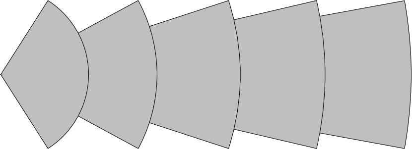
Figure 5.— Illustration of an optimal survey design with multi-layers of regions.

The optimal survey illustrated here consists of several layers of sub-surveys. Each sub-survey is optimized to catalog particular redshift range and has selection criteria that is most effective to pick the galaxies up in corresponding range of redshift. While simple color selections can be used for this purpose, the photometric redshift data might be the best to fulfill the required selections. In low-redshift layers, the surface number density of galaxies for the spectroscopy can be low, while the sky coverage of the survey regions should be wide. In high-redshift layers, the surface number density should be high, while the sky coverage can be narrow. The requirements of the telescope for each layers are different. Thus this optimal survey would effectively carried out by several telescopes with a wide spectrum of capabilities such as resolutions and wideness of the field of view.

One can also imagine a limit of infinite number of layers. The survey geometry in this case is like a big column in redshift space, as illustrated in Figure 6.

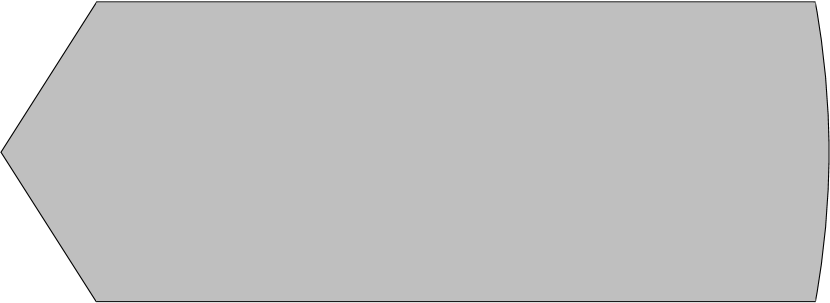
Figure 6.— Another survey design with continuous layers.

In this case, the selection criteria should continuously vary with the position on the sky, therefore delicate selections are required to sample galaxies as homogeneously as possible. While technically more challenging, this survey strategy is ideal for the cosmological analysis of the clustering at various redshifts in the deep universe.

In this section, however, we consider more realistic surveys that can be achieved by present-day technologies. We take the series of baseline redshift surveys explained below. The surveys are categorized to four types, which are assumed to be volume-limited samples. The choices of samples at high-redshifts are similar to that considered by Seo & Eisenstein (2003).

The first sample is a low-redshift sample around $z\sim 0.15$. This sample is motivated by a volume-limited subsample of galaxies in the SDSS survey (Tegmark et al., 2004) with absolute $r$-magnitude $M_{r}\sim-22$. Our baseline sample has a uniform number density $\bar{n}=1\times 10^{-3}/({\hbox{$\,h^{-1}$}{\rm Mpc}})^{3}$ in the redshift range $z=0.05$–$0.25$. The sky coverage is assumed to be ${\mit\Omega}_{\rm sky}=8.05$ str. The bias factor is assumed to be $b=1.3$. We call this sample as Sample A below.

The second sample is the one around $z\sim 0.3$. This sample is motivated by the volume-limited catalog of the Luminous Red Galaxies (LRGs) in the SDSS survey (Eisenstein et al., 2001). Our sample is assumed to have $\bar{n}=1\times 10^{-4}/({\hbox{$\,h^{-1}$}{\rm Mpc}})^{3}$, $z=0.2$–$0.4$, ${\mit\Omega}_{\rm sky}=2.57$ str., and $b=2.0$. We call this sample as Sample B below.

The next samples are the series of surveys around $z\sim 1$. The choice of the target galaxies is not trivial. We follow the baseline surveys that are considered by Seo & Eisenstein (2003). The target galaxies are assumed to be either giant ellipticals or luminous star-forming galaxies. This category of samples consists of surveys of four redshift bins, $z=0.5$–$0.7$, $z=0.7$–$0.9$, $z=0.9$–$1.1$, and $z=1.1$–$1.3$. The sky coverage is assumed to be ${\mit\Omega}_{\rm sky}=0.914$, $0.647$, $0.517$, and $0.451$, respectively. The bias factors are $1.25$, $1.40$, $1.55$, and $1.70$, respectively. Approximately we have $\sigma_{\rm 8g}\simeq 1$ in each samples with the above choices of bias factors. We assume $\bar{n}=5\times 10^{-4}/({\hbox{$\,h^{-1}$}{\rm Mpc}})^{3}$ commonly for each samples. We call the series of samples as Sample C1 to Sample C4 below.

The last sample is the survey of Lyman break galaxies around $z\sim 3$. The selection techniques for this kind of galaxies are reported by Steidel et al. (1996). We consider the sample with a redshift range of $z=2.65$–$3.35$. We assume $b=3.3$ and $\bar{n}=1\times 10^{-3}/({\hbox{$\,h^{-1}$}{\rm Mpc}})^{3}$ which are consistent with the observation (Steidel et al., 1998; Adelberger et al., 1998). We call this sample as Sample D. The parameters of the baseline surveys are summarized in Table 1.

Table 1Parameters of the baseline surveys.

Samples	$z$	area [str.]	$b$	$\bar{n}$ [$/(10{\hbox{$\,h^{-1}$}{\rm Mpc}})^{3}$]	Candidates
A	0.05–0.25	8.05	1.30	$1.0$	$M_{r}\sim-22$ galaxies
B	0.2–0.4	2.57	2.00	$0.1$	Luminous red galaxies
C1	0.5–0.7	0.914	1.25	$0.5$
C2	0.7–0.9	0.647	1.40	$0.5$	Giant ellipticals, or
C3	0.9–1.1	0.517	1.55	$0.5$	star-forming galaxies
C4	1.1–1.3	0.451	1.70	$0.5$
D	2.65–3.35	0.102	3.30	$1.0$	Lyman break galaxies

The Fisher matrix is calculated by assuming a cone geometry with an open angle which gives 1/10 of the assumed sky coverage in each sample. The spherical cells with a comoving radius $15{\hbox{$\,h^{-1}$}{\rm Mpc}}$ are placed in closed-packed structure in a survey region. The total number of cells is exactly 4900 in each 1/10 subsample. Thus the comoving volumes of all samples are essentially the same. The resulting Fisher matrix is multiplied by 10 to obtain the final Fisher matrix. This method of subdividing the sample into 1/10 is taken to reduce the dimension of the matrix and to compromise with the CPU time and the memory requirement of handling the large correlation matrix. In general, the subdivision overestimates the error bounds because the information from cross correlations between subsamples is neglected. However, the larger the sample is, the less such cross correlations are. We confirmed that the error bounds of the full sample is accurately calculated by just adding the Fisher matrices of the subsamples in our case.

4.3. Results of the Fisher Analysis

According to the calculation of the Fisher matrix, the expected error bounds with any marginalization are straightforwardly obtained by methods explained in Appendix B. Since the bias parameter should be simultaneously determined sample by sample, we calculate the Fisher matrix of each sample with bias separately marginalized over within each sample. Therefore, the results below are not affected by bias uncertainties, as long as the bias factor does not significantly varies within each samples.

In Figure 7, concentration ellipsoids in 2-parameter estimations are plotted, i.e., each panel shows the expected error bounds when corresponding two parameters are simultaneously determined, fixing other parameters except the bias parameter.

Figure 7.— Two-parameter joint error bounds expected by the baseline surveys. Each ellipse represents the expected constraint on the parameter space with $1\sigma$ significance. In each panel, corresponding two parameters are varied with bias marginalized over. Other parameters are fixed in each plot. Error bounds for Sample A (dotted lines), Sample B (short-dashed lines), Sample C1–C4 (long-dashed lines), Sample D (dot-dashed lines) are plotted together with a combined sample (solid lines).

The bias parameters are marginalized over. The Fisher matrix of the combined sample are also calculated by adding the Fisher matrices of Sample A–D with bias separately marginalized over sample by sample.

Most of the pairs of parameters do not exhibit degeneracy between them. This means that those pairs of parameters contribute to the correlation function fairly differently as explained in §3. However, one can notice relatively clear degeneracies between ${\mit\Omega}_{\rm K0}$ and $w$. Since we consider ${\mit\Omega}_{\rm M0}$ and ${\mit\Omega}_{\rm K0}$ as independent parameters, changing the parameter ${\mit\Omega}_{\rm K0}$ is equivalent to changing the dark energy density ${\mit\Omega}_{\rm Q0}$ with ${\mit\Omega}_{\rm M0}$ fixed. The parameters of the dark energy are mainly constrained by AP effect besides the linear growth rate. In the low-redshift samples, the parameters ${\mit\Omega}_{\rm Q0}$ and $w$ only depend on the growth rate and thus degenerate with each other. Since the bias parameter and the growth rate is distinguishable by the velocity distortion, one can still extract information on the dark energy from low-redshift sample with the cost of the degeneracy. On the other hand, high-redshift samples can actually constrain these two dark energy parameter independently.

The direction of the major axis of the concentration ellipse in the ${\mit\Omega}_{\rm K0}$–$w$ plane rotates anti-clockwise with the average redshift of the samples. Accordingly, the concentration ellipse of the combined sample is quite small. For example, the error bound of ${\mit\Omega}_{\rm Q0}$ is $\sim\pm 2\%$ and that of $w$ is $\sim\pm 5\%$. The presented error bounds are given when the other parameters are fixed except the bias. It is also interesting to see the expected constraints when all parameters are determined by only using the deep galaxy surveys. In Figure 8, the concentration ellipses are plotted on ${\mit\Omega}_{\rm K0}$–$w$ plane when the other parameters ${\mit\Omega}_{\rm M0}$, ${\mit\Omega}_{\rm M0}h$, $f_{\rm B}$, $\sigma_{8}$ and $b$’s are all marginalized over.

Figure 8.— Joint error bounds of the dark energy parameters expected by the baseline surveys. Parameters ${\mit\Omega}_{\rm M0}$, ${\mit\Omega}_{\rm M0}h$, $f_{\rm B}$, $\sigma_{8}$ and $b$ are all marginalized over. The correspondences between lines and samples are the same as in Figure 7.

The complementarity of the surveys at various redshifts is obvious in this case. The concentration ellipses of high-redshift samples are also elongated by uncertainties of other parameters. The direction of the major axis of the ellipses rotates anti-clockwise with redshifts. Consequently, the degeneracy between ${\mit\Omega}_{\rm K0}$ and $w$ are broken in the combined sample and the error bound is much smaller than in the individual samples. The error bound of ${\mit\Omega}_{\rm Q0}$ is $\sim\pm 4\%$ and that of $w$ is $\sim\pm 10\%$ even when all the other parameters are completely unknown.

5. Conclusions and Discussion

In this paper, properties of the two-point correlation function in deep redshift space is theoretically investigated. A completely general expression of the linear correlation function derived by Matsubara (2000) is reduced to a simpler form, eq.(1)–(16) with an approximation which is valid for realistic surveys. Baryon wiggles in the power spectrum correspond to a single peak in the correlation function. This peak differently depends on the parameters of the underlying power spectrum, ${\mit\Omega}_{M0}h$, $f_{\rm B}$, and $h$. In the two-dimensional contour plot of the correlation function in redshift space, the corresponding feature is the baryonic ridge. The shape of the ridge is perfectly circular in comoving space, in spite of the effects of the peculiar velocity. This is preferable for the cosmological test by the AP effect. Using the analysis of the Fisher information matrix, the cosmological test by the correlation function in deep redshift space is shown to constrain the properties of the dark energy component as well as other cosmological parameters, even if the bias is uncertain. In particular, there is a clear complementarity of the samples of various redshift ranges in probing the dark energy component.

Therefore, a survey of a wide redshift range is particularly useful to probe the dark energy. Keeping a sufficient number density of galaxies in the given observation time, examples of the optimally designed survey geometry are illustrated in Figure 5 and Figure 6. Selecting galaxies for the spectroscopic follow-ups as densely as possible is one of the major technical challenges in this kind of survey strategy. However, recent advances of the technology enable us to carry it out. With the advent of 8-10m telescopes, galaxies of $z\lower 2.15277pt\hbox{$\;\buildrel<\over{\sim}\;$}1.4$ can be straightforwardly selected by color selections as demonstrated by, e.g., the SDSS survey (York et al., 2000; Eisenstein & Hu, 1998) and the DEEP2 Galaxy Redshift Survey (Davis et al., 2003; Coil et al., 2003). In $z\lower 2.15277pt\hbox{$\;\buildrel>\over{\sim}\;$}2.5$, Lyman-break galaxies are photometrically selected with sufficient density (Steidel et al., 1996, 1998; Adelberger et al., 1998). The range $1.4\lower 2.15277pt\hbox{$\;\buildrel<\over{\sim}\;$}z\lower 2.15277pt\hbox{$\;\buildrel<\over{\sim}\;$}2.5$ is known as the redshift desert, since spectroscopic identifications of galaxies were historically difficult. Recently, Steidel et al. (2004) showed that large numbers of galaxies in this range can actually be selected with standard broadband color selection technique using the Keck I Telescope with the LRIS-B spectrograph. Thus galaxies at $z\lower 2.15277pt\hbox{$\;\buildrel<\over{\sim}\;$}3$ can be optically selected by ground-based 8-10m telescopes with sufficient number densities (Adelberger et al., 2004). Therefore, the proposed surveys illustrated by Figure 5 and Figure 6 in the redshift range of $z\lower 2.15277pt\hbox{$\;\buildrel<\over{\sim}\;$}3$ with approximately homogeneous selections are accessible by present-day technologies.

Cosmology with the large-scale structure has mainly been studied by the snapshot of the nearly present universe, since the sufficient number of galaxies have been available only at shallow redshifts, $z\lower 2.15277pt\hbox{$\;\buildrel<\over{\sim}\;$}0.3$. CMB observations, on the other hand, map the universe of the $z\simeq 1100$ universe. The observations of the galaxy clustering in the deep-redshift universe of $0.3\lower 2.15277pt\hbox{$\;\buildrel<\over{\sim}\;$}z\lower 2.15277pt\hbox{$\;\buildrel<\over{\sim}\;$}3$, which are within reach of the present-day technology, will provide a unique information on the evolving universe with the analysis of the correlation function presented in this paper. Observations of the evolving universe is momentous not only to probe the nature of the dark energy component of the universe, but also to establish or even falsify the standard picture of the cosmology. Only data of the snapshots of the universe are not enough to confirm the consistency of the cosmological model. Whether or not the structure of the universe with respect to both space and time are fully explained by minimal set of cosmological assumptions and parameters will be a major concern in cosmology. In the era of the precision cosmology, any need for additional assumptions will suggest terra incognita in the physical universe.

Appendix A Basic Notations

In this Appendix, basic notations of the Friedmann-Lemaître universe with dark energy extension used in this paper are introduced.

The background metric is given by the Robertson-Walker metric,

$$ds^{2}=-dt^{2}+a^{2}(t)\left[dx^{2}+{S_{K}}^{2}(x)\left(d\theta^{2}+\sin^{2}\theta\phi^{2}\right)\right],$$ (A1)

where we employ a unit system with $c=1$, and adopt a notation,

$$S_{K}(x)\equiv\left\{\begin{array}[]{ll}(-K)^{-1/2}{\rm sinh}\left[(-K)^{1/2}x\right],&(K<0),\\ x,&(K=0),\\ K^{-1/2}\sin\left[K^{1/2}x\right],&(K>0),\end{array}\right.$$ (A2)

where $K$ is the spatial curvature of the universe. The comoving distance $x(z)$ at redshift $z$ is given by

$$x(z)=\int_{0}^{z}\frac{dz^{\prime}}{H(z^{\prime})},$$ (A3)

where $H(z)$ is the redshift-dependent Hubble parameter. When we allow the dark energy component having a non-trivial equation of state, $p(z)=w(z)\rho(z)$, the Hubble parameter is given by

$$H(z)=H_{0}\left[(1+z)^{3}{\mit\Omega}_{\rm M0}-(1+z)^{2}{\mit\Omega}_{\rm K0}+\exp\left(3\int_{0}^{z}\frac{1+w}{1+z}dz\right){\mit\Omega}_{\rm Q0}\right]^{1/2},$$ (A4)

where ${\mit\Omega}_{\rm M0}$ is the density parameter of matter, ${\mit\Omega}_{\rm Q0}$ is the density parameter of dark energy, and ${\mit\Omega}_{\rm K0}={\mit\Omega}_{\rm M0}+{\mit\Omega}_{\rm Q0}-1$ is the curvature parameter. The linear growth factor $D(z)$ and its logarithmic derivative, $f(z)\equiv d\ln D/d\ln a=-(1+z)d\ln D/dz$ are the solution of the following simultaneous differential equations (Matsubara & Szalay, 2003)

$$\frac{d\ln D}{d\ln a}=f,$$ (A5)

$$\frac{df}{d\ln a}=-f^{2}-\left(1-\frac{{\mit\Omega}_{\rm M}}{2}-\frac{1+3w}{2}{\mit\Omega}_{\rm Q}\right)f+\frac{3}{2}{\mit\Omega}_{\rm M},$$ (A6)

where the scale factor $a$ is related to the redshift by $a=(1+z)^{-1}$, and ${\mit\Omega}_{\rm M}$, ${\mit\Omega}_{\rm Q}$ are the time-dependent density parameters of matter and dark energy, respectively:

$${\mit\Omega}_{\rm M}(z)=\frac{{H_{0}}^{2}}{H^{2}(z)}(1+z)^{3}{\mit\Omega}_{\rm M0}$$ (A7)

$${\mit\Omega}_{\rm Q}(z)=\frac{{H_{0}}^{2}}{H^{2}(z)}\exp\left(3\int_{0}^{z}\frac{1+w}{1+z}dz\right){\mit\Omega}_{\rm Q0}$$ (A8)

The normalization $D(z=0)=1$ is adopted throughout this paper.

Appendix B Marginalized Fisher Matrix

In this Appendix, useful equations to obtain estimates of the error covariance from the Fisher matrix when some parameters are marginalized over. The Fisher matrix $F$ is an expectation value of the curvature matrix of the logarithmic likelihood function in parameter space,

$$F_{\alpha\beta}({\mbox{\boldmath$\theta$}})=-\left\langle\frac{\partial^{2}\ln{\cal L}}{\partial\theta_{\alpha}\partial\theta_{\beta}}\right\rangle,$$ (B1)

where ${\mbox{\boldmath$\theta$}}=(\theta_{1},\theta_{2},\ldots)^{\rm T}$ is a set of model parameters, and ${\cal L}$ is the likelihood function. In the Fisher matrix analysis, the error covariance matrix $\langle\Delta{\mbox{\boldmath$\theta$}}\Delta{\mbox{\boldmath$\theta$}}^{\rm T}\rangle$ of a set of model parameters asymptotically corresponds to the inverse of the Fisher matrix

$$F^{-1}\simeq\langle\Delta{\mbox{\boldmath$\theta$}}\Delta{\mbox{\boldmath$\theta$}}^{\rm T}\rangle,$$ (B2)

when all the parameters are simultaneously determined.

The error covariance matrix of partial set of parameters, marginalizing over other parameters is given by a sub-matrix of the inverse of the Fisher matrix. Therefore, a Fisher matrix $\widetilde{F}$ of these partial set of parameters corresponds to the inverse of the sub-matrix of equation (B2). We consider the situation that the first $n$ parameters are estimated and other $m$ parameters are marginalized over. The full Fisher matrix has a form,

$$F=\left(\begin{array}[]{cc}A&B\\ B^{\rm T}&C\\ \end{array}\right)$$ (B3)

where $A$ is an $n\times n$ symmetric matrix, $B$ is an $n\times m$ matrix, and $C$ is an $m\times m$ symmetric matrix. A representation of the inverse of the equation (B4) is given by

$$F^{-1}=\left(\begin{array}[]{cc}\left(A-BC^{-1}B^{\rm T}\right)^{-1}&-\left(A-BC^{-1}B^{\rm T}\right)^{-1}BC^{-1}\\ -\left(C-B^{\rm T}A^{-1}B\right)^{-1}B^{\rm T}A^{-1}&\left(C-B^{\rm T}A^{-1}B\right)^{-1}\\ \end{array}\right),$$ (B4)

as can be explicitly confirmed that $F^{-1}F=I$. Therefore, the marginalized $n\times n$ Fisher matrix $\widetilde{F}$ of the reduced parameters corresponds to

$$\widetilde{F}=A-BC^{-1}B^{\rm T}.$$ (B5)

The first term is the Fisher matrix of the reduced parameter space, without marginalization, and the second term corresponds to the effects of the marginalization.

Given a Fisher matrix $\widetilde{F}$, with or without marginalization, the estimations of the error bounds are obtained by contours of concentration ellipsoid $\Delta{\mbox{\boldmath$\theta$}}^{\rm T}\widetilde{F}\Delta{\mbox{\boldmath$\theta$}}={\rm const.}$, where ${\rm const.}$ depends on significance levels and dimensionality of the parameter space. Therefore, obtaining the marginalized Fisher matrix by the equation (B5) is sufficient to obtain the error estimation by drawing concentration ellipsoids, and calculation of an inverse of the full Fisher matrix is not necessary.

Below, we derive the correspondence between contour levels of $\Delta{\mbox{\boldmath$\theta$}}^{\rm T}\widetilde{F}\Delta{\mbox{\boldmath$\theta$}}$ and the significance level in the joint estimation of multiple parameters. Assuming a Gaussian profile around a peak of the likelihood function, and the correspondence between covariance matrix and the Fisher matrix of equation (B2), an estimate of $\nu\sigma$ error bounds can be obtained by solving an equation for $X(\nu)$,

$$\left[(2\pi)^{n}\det\widetilde{F}^{-1}\right]^{-1/2}\int_{\Delta{\mbox{\scriptsize\boldmath$\theta$}}^{\rm T}\widetilde{F}\Delta{\mbox{\scriptsize\boldmath$\theta$}}\leq X^{2}}d^{n}\theta\exp(-\frac{1}{2}\Delta{\mbox{\boldmath$\theta$}}^{\rm T}\widetilde{F}\Delta{\mbox{\boldmath$\theta$}})=\frac{1}{\sqrt{2\pi}}\int_{-\nu}^{\nu}e^{-t^{2}/2},$$ (B6)

where

$$\Delta{\mbox{\boldmath$\theta$}}^{\rm T}\widetilde{F}\Delta{\mbox{\boldmath$\theta$}}=X^{2}(\nu)$$ (B7)

defines a concentration ellipsoid of $\nu\sigma$ significance level. Adopting a linear transformation of variables, ${\mbox{\boldmath$x$}}=L^{\rm T}\Delta{\mbox{\boldmath$\theta$}}$, where $L$ is a $n\times n$ matrix by a Cholesky decomposition of the Fisher matrix, $\widetilde{F}=LL^{\rm T}$, the equation (B6) reduces to a simple equation,

$$\int_{0}^{X}dxx^{n-1}e^{-x^{2}/2}=2^{n/2-1}{\mit\Gamma}\left(n/2\right){\rm erf}\left(\nu/\sqrt{2}\right),$$ (B8)

where ${\rm erf}(x)=2\pi^{-1/2}\int_{0}^{x}dte^{-t^{2}}$ is the error function. Numerical solutions of this equation in several cases are given in Table 2.

Table 2Contour levels $X(\nu)$ of the concentration ellipsoids in joint estimations of parameters.

	$n=1$	$n=2$	$n=3$
$\nu=1$	$1$	$1.52$	$2.17$
$\nu=2$	$2$	$2.49$	$3.12$
$\nu=3$	$3$	$3.44$	$4.03$

In this paper, $1\sigma$ concentration ellipses in marginalized 2-parameter space are presented, i.e., $n=2$, $\nu=1$ and $X=1.52$.

References

- Adelberger et al. (1998) Adelberger, K. L., Steidel, C. C., Giavalisco, M., Dickinson, M., Pettini, M., & Kellogg, M. 1998, ApJ, 505, 18
- Adelberger et al. (2004) Adelberger, K. L., Steidel, C. C., Shapley, A. E., Hunt, M. P., Erb, D. K., Reddy, N. A., & Pettini, M. 2004, ApJ, 607, 226
- Alcock & Paczyński (1979) Alcock, C. & Paczyński, B. 1979, Nature, 281, 358
- Ballinger, Peacock & Heavens (1996) Ballinger, W. E. & Peacock, J. A. & Heavens, A. F. 1996, MNRAS, 282, 877
- Bennett et al. (2003) Bennett, C. L. et al. 2003, ApJS, 148, 1
- Blake & Glazebrook (2003) Blake, C. & Glazebrook, K. 2003, ApJ, 594, 665
- Coil et al. (2003) Coil, A. L., et al. 2003, ApJ, in press (ArXiv astro-ph/0305586)
- Colless et al. (2001) Colless, M. et al. 2001, MNRAS, 328, 1039
- Davis et al. (2003) Davis, M., et al. 2003, Proc. SPIE, 4834, 161 (ArXiv astro-ph/0209419)
- Eisenstein & Hu (1998) Eisenstein, D. J. & Hu, W. 1998, ApJ, 496, 605
- Eisenstein et al. (2001) Eisenstein, D. J. et al. 2001, AJ, 122, 2267
- Hamilton (1992) Hamilton, A. J. S. 1992, ApJ, 385, L5
- Hu & Haiman (2003) Hu, W. & Haiman, Z. 2003, Phys. Rev. D, 68, 063004
- Kaiser (1987) Kaiser, N. 1987, MNRAS, 227, 1
- Kendall & Stuart (1969) Kendall, M. G. & Stuart, A. 1969, The Advanced Theory of Statistics, Vol. 2 (London: Griffin)
- Linder (2003) Linder, E. V. 2003, Phys. Rev. D, 68, 083504
- Mather et al. (1999) Mather, J. C., Fixsen, D. J., Shafer, R. A., Mosier, C., & Wilkinson, D. T. 1999, ApJ, 512, 511
- Matsubara (1999) Matsubara, T. 1999, ApJ, 525, 543
- Matsubara (2000) Matsubara, T. 2000, ApJ, 535, 1
- Matsubara, Szalay, & Pope (2004) Matsubara, T., Szalay, A. S., & Pope, A. C. 2004, ApJ, in press (ArXiv: astro-ph/0401251)
- Matsubara & Suto (1996) Matsubara, T. & Suto, Y. 1996, ApJ, 470, L1
- Matsubara & Szalay (2002) Matsubara, T. & Szalay, A. S. 2002, ApJ, 574, 1
- Matsubara & Szalay (2003) Matsubara, T. & Szalay, A. S. 2003, Physical Review Letters, 90, 021302
- Peebles (1980) Peebles, P. J. E. 1980, The Large-Scale Structure of the Universe (Princeton; Princeton University Press)
- Perlmutter et al. (1999) Perlmutter, S. et al. 1999, ApJ, 517, 565
- Riess et al. (1998) Riess, A. G. et al. 1998, AJ, 116, 1009
- Saunders et al. (2000) Saunders, W. et al. 2000, MNRAS, 317, 55
- Scherrer & Weinberg (1998) Scherrer, R. J. & Weinberg, D. H. 1998, ApJ, 504, 607
- Seo & Eisenstein (2003) Seo, H. & Eisenstein, D. J. 2003, ApJ, 598, 720
- Shectman et al. (1996) Shectman, S. A., Landy, S. D., Oemler, A., Tucker, D. L., Lin, H., Kirshner, R. P., & Schechter, P. L. 1996, ApJ, 470, 172
- Spergel et al. (2003) Spergel, D. N. et al. 2003, ApJS, 148, 175
- Steidel et al. (1996) Steidel, C. C., Giavalisco, M., Pettini, M., Dickinson, M., & Adelberger, K. L. 1996, ApJ, 462, L17
- Steidel et al. (1998) Steidel, C. C., Adelberger, K. L., Dickinson, M., Giavalisco, M., Pettini, M., & Kellogg, M. 1998, ApJ, 492, 428
- Steidel et al. (2004) Steidel, C. C., Shapley, A. E., Pettini, M., Adelberger, K. L., Erb, D. K., Reddy, N. A., & Hunt, M. P. 2004, ApJ, 604, 534 (ArXiv: astro-ph/0401439)
- Szalay, Matsubara & Landy (1998) Szalay, A. S., Matsubara, T., & Landy, S. D. 1998, ApJ, 498, L1
- Tegmark, Taylor & Heavens (1997) Tegmark, M., Taylor, A. N., & Heavens, A. F. 1997, ApJ, 480, 22
- Tegmark et al. (2004) Tegmark, M., et al. 2004, ApJ, 606, 702
- Therrien (1992) Therrien, C. W. 1992, Discrete Random Signals and Statistical Signal Processing, (New Jersey: Prentice-Hall).
- Vogeley & Szalay (1996) Vogeley, M. S. & Szalay, A. S. 1996, ApJ, 465, 34
- York et al. (2000) York, D. G. et al. 2000, AJ, 120, 1579