Some Like it Hot: The X-Ray Emission of The Giant Star YY Mensae

Abstract

We present an analysis of the X-ray emission of the rapidly rotating giant star YY Mensae (catalog ) observed by Chandra  HETGS and XMM-Newton. The high-resolution spectra display numerous emission lines of highly ionized species; Fe XVII to Fe XXV lines are detected, together with H-like and He-like transitions of lower $Z$ elements. Although no obvious flare was detected, the X-ray luminosity changed by a factor of two between the XMM-Newton  and Chandra  observations taken 4 months apart (from $\log L_{X}\approx 32.2$ to $32.5$ erg s^-1, respectively). The coronal abundances and the emission measure distribution have been derived from three different methods using optically thin collisional ionization equilibrium models, which is justified by the absence of opacity effects in YY Men as measured from line ratios of Fe XVII transitions. The abundances show a distinct pattern as a function of the first ionization potential (FIP) suggestive of an inverse FIP effect as seen in several active RS CVn binaries. The low-FIP elements ($<10$ eV) are depleted relative to the high-FIP elements; when compared to its photospheric abundance, the coronal Fe abundance also appears depleted. We find a high N abundance in YY Men’s corona which we interpret as a signature of material processed in the CNO cycle and dredged-up in the giant phase. The corona is dominated by a very high temperature ($20-40$ MK) plasma, which places YY Men among the magnetically active stars with the hottest coronae. Lower temperature plasma also coexists, albeit with much lower emission measure. Line broadening is reported in some lines, with a particularly strong significance in Ne X Ly$\alpha$. We interpret such a broadening as Doppler thermal broadening, although rotational broadening due to X-ray emitting material high above the surface could be present as well. We use two different formalisms to discuss the shape of the emission measure distribution. The first one infers the properties of coronal loops, whereas the second formalism uses flares as a statistical ensemble. We find that most of the loops in the corona of YY Men have their maximum temperature equal to or slightly larger than about $30$ MK. We also find that small flares could contribute significantly to the coronal heating in YY Men. Although there is no evidence of flare variability in the X-ray light curves, we argue that YY Men’s distance and X-ray brightness does not allow us to detect flares with peak luminosities $L_{\mathrm{X}}\leq 10^{31}$ erg s^-1 with current detectors.

1. Introduction

Magnetic activity is ubiquitous in late-type stars, although its level can vary dramatically. A common activity indicator is the ratio of the X-ray luminosity to the stellar bolometric luminosity, $L_{\mathrm{X}}/L_{\mathrm{bol}}$; it varies typically from $10^{-7}$ in inactive stars to $10^{-3}-10^{-2}$ in the most active stars (see, e.g., Favata & Micela 2003 and Güdel 2004 for recent reviews on the X-ray emission of stellar coronae). Giant stars present a peculiar behavior in which magnetic activity is strong for spectral types earlier than typically K0-2 III, while it vanishes rapidly for cooler spectral types (e.g., Linsky & Haisch, 1979; Ayres et al., 1981; Linsky, 1985; Hünsch et al., 1996, and references therein). Rotational breaking occurs in giants around spectral type G0 III (Gray, 1989). Although the origin of the divide remains debated, Hünsch & Schröder (1996) suggested that the evolutionary history of magnetically active stars of different masses explains the X-ray dividing line (also Schröder, Hünsch, & Schmitt, 1998). Alternatively, Rosner et al. (1995) proposed that the dividing line could be explained by the change from a predominantly closed magnetic configuration in stars blueward of the dividing line to a predominantly open configuration in cooler giants. The latter configuration induces cool winds and the absence of hot coronae. Holzwarth & Schüssler (2001) argued that flux tubes in giants of spectral types G7 to K0 remain inside the stellar convection zone in a stable equilibrium.

FK Comae stars form a loosely-defined class of rapidly rotating single G and K giant stars, whose outstanding property is a projected equatorial velocity measured up to 160 km s^-1, in contrast to the expected maximum of 6 km s^-1  for giants. One of the leading theories to explain the extreme properties of FK Com stars suggests that they were formed by coalescence of a contact binary when one of the components entered into the giant stage (Bopp & Rucinski, 1981a; Bopp & Stencel, 1981b; Rucinski, 1990). Simon & Drake (1989) noted alternatively that dredge-up of angular momentum during the early red giant phase could explain their rapid rotation. Magnetic activity in FK Com stars is very strong (Bopp & Stencel, 1981b; Fekel et al., 1986; Rutten, 1987; Simon & Drake, 1989). In the X-ray regime, their X-ray luminosities are in the range from $L_{\mathrm{X}}=10^{30}$ to $10^{31}$ erg s^-1, i.e., $L_{\mathrm{X}}/L_{\mathrm{bol}}\sim 10^{-5}-10^{-3}$ (e.g., Maggio et al., 1990; Welty & Ramsey, 1994; de Meideros & Mayor, 1995; Huenemoerder, 1996; Hünsch, Schmitt, & Voges, 1998; Gondoin, 1999; Gondoin, Erd, & Lumb, 2002).

We present in this paper new high-resolution X-ray spectra and high signal-to-noise light curves of the FK Com-type star YY Mensae (catalog ) (HD 32918 (catalog )) obtained with the Chandra X-ray Observatory and its High-Energy Transmission Grating Spectrometer (HETGS), and with the XMM-Newton Observatory. With these observations, we aimed to compare the X-ray emission of this bright FK Com-type star with that of other magnetically active stars. We show that YY Men is among the stars with the hottest coronae, with a dominant plasma temperature around $20-40$ MK. Furthermore, we investigated the elemental composition of YY Men’s corona to study abundance anomalies.

The paper is structured as follows: Section 2 describes the main properties of YY Men and previous observations; section 3 gives the observation details, whereas the data reduction is described in section 4 (Sect. 4.1 for Chandra  and Sect. 4.2 for XMM-Newton). In section 5, we provide an analysis of the light curves. Section 6 describes the procedures for our spectral analysis for Chandra  (Sect. 6.1) and XMM-Newton  (Sect. 6.2). We approached the spectral inversion problem with three different methods to obtain the emission measure distribution (EMD) and abundances in YY Men’s corona (Sect. 6.3). Section 7 includes a discussion of our results: abundances (Sect. 7.1), EMD (Sect. 7.2), line broadening (Sect. 7.3), electron densities (Sect. 7.4), and optical depth effects (Sect. 7.5). Finally, we give a summary and our conclusions in section 8.

2. The Giant Star YY Mensae

YY Mensae (catalog ) (K1 IIIp) is a strong Ca II emitter (Bidelman & MacConnell, 1973) at a distance of $291$ pc (Perryman et al., 1997), with a mass of $M=2.2~{}M_{\sun}$ (see Gondoin, 1999), and a radius of $R=8.8\times 10^{11}$ cm = $12.7R_{\sun}$, based on $T_{\mathrm{eff}}=4,700$ K from Randich, Gratton, & Pallavicini (1993) and $L_{\mathrm{bol}}=2.7\times 10^{35}$ erg s^-1 $=70L_{\sun}$ from Cutispoto et al. (1992). It belongs to the FK Com-type class of giant stars (Collier Cameron, 1982). It displays a photometric period of $P=9.55$ days, a projected rotational velocity of $v\sin i=45-50$ km s^-1  (Collier Cameron, 1982; Piskunov, Tuominen, & Vilhu, 1990; Glebocki & Stawikowski, 2000), and an inclination angle of $i=65\arcdeg$ (Piskunov et al., 1990). Grewing, Bianchi, & Cassatella (1986) presented the IUE ultraviolet spectrum of YY Men (catalog ), showing very strong ultraviolet (UV) emission lines originating from the chromosphere and the transition zone. They obtained YY Men’s EMD in the range $\log T(\mathrm{K})=3.8-5.3$, emphasizing its strength in comparison to other magnetically active stars. Line ratios indicated characteristic electron densities in the transition zone of $n_{e}=3-4\times 10^{10}$ cm^-3  (Grewing et al., 1986). Strong flares were observed in the radio and optical, lasting for several days (Slee et al., 1987; Bunton et al., 1989; Cutispoto, Pagano, & Rodono, 1992). A strong P Cyg profile in the H$\alpha$ line during a flare indicated strong outflowing material with a velocity of $230$ km s^-1  (Bunton et al., 1989). Finally, spot coverage in YY Men was generally found in an equatorial belt (Piskunov et al., 1990), in contrast to the large polar caps found in many active stars (e.g., Vogt, 1988).

In the X-ray regime, Bedford, Elliott, & Eyles (1985) reported X-rays from YY Men detected with the EXOSAT CMA instrument. Güdel et al. (1996) gave results of observations made with ROSAT and ASCA. They found indications for a hot (up to 3 keV) dominant coronal plasma. Flaring activity was reported, although hampered by many interruptions due to the low orbits of the satellites. Abundance depletion in most elements was suggested from fits to the medium-resolution ASCA spectra. The X-ray luminosities varied between the observations and ranged from $\log L_{\mathrm{X}}=32.3$ to $32.65$ erg s^-1  (Güdel et al., 1996).

Our Chandra and XMM-Newton observations are generally consistent with the above results. Nevertheless, deep, uninterrupted monitoring and high spectral resolution provide the opportunity to significantly improve our understanding of the corona of YY Men.

3. Observations

Chandra  and XMM-Newton  observed YY Men as part of Cycle 4 and of the Reflection Grating Spectrometer (RGS) Guaranteed Time, respectively. We provide a log of the observations in Table 1.

Chandra  observed the giant with the Advanced CCD Imaging Spectrometer (ACIS) in its 1x6 array (ACIS-S) with the HETG inserted (Weisskopf et al., 2002). This configuration provides high-resolution X-ray spectra from 1.2 to 16 Å  for the High-Energy Grating (HEG) spectrum and from 2.5 to 31 Å  for the Medium-Energy Grating (MEG) spectrum. The HETGS has constant resolution (HEG: $\Delta\lambda\sim 12$ mÅ, MEG: $\Delta\lambda\sim 23$ mÅ  FWHM). Thanks to the energy resolution of the ACIS camera, spectral orders can be separated. However, because of the drop in effective area with higher spectral orders, we used only the first-order spectra. Further details on the instruments can be found in the Chandra Proposers' Observatory Guide.

XMM-Newton  (Jansen et al., 2001) observed YY Men in the X-rays with the RGS ($\lambda\sim 6-38$ Å  with $\Delta\lambda\sim 60-76$ mÅ; den Herder et al. 2001) and the European Photon Imaging Camera (EPIC) MOS only ($0.15-10$ keV with $E/\Delta E=20-50$; Turner et al. 2001), since the EPIC pn camera (Strüder et al., 2001) was off-line due to a sudden switching off of one quadrant . Simultaneous optical coverage was obtained with the Optical Monitor (OM; Mason et al., 2001), although we did not make use of the data because YY Men was too bright ($V=8.1$) for the $U\!$ filter. Furthermore, we note that, due to a small pointing misalignment, YY Men fell off the small $11\arcsec\times 11\farcs 5$ timing window.

4. Data Reduction

4.1. The Chandra  data

The Chandra  data were reduced with the Chandra  Interactive Analysis of Observations (CIAO) version 2.3 in conjunction with the calibration database (CALDB) 2.21. We started from the level 1 event file. We used standard techniques described in analysis threads. In particular, we applied a correction for charge transfer inefficiency, applied pulse height analysis and pixel randomizations, and we destreaked CCD 8 (ACIS-S4). Furthermore, we used non-default masks and background spectral extraction masks to reflect the modifications introduced in the recent CIAO 3 release.

We then calculated grating response matrix files (RMFs) and grating ancillary response files (ARFs). CALDB 2.21 contained separate line spread functions (LSF) for the positive and the negative order spectra. We then co-added the positive and negative order spectra to increase statistics (using the co-added grating ARFs), and further binned the spectra by a factor of two. Our final HEG and MEG first-order spectra have bin widths of 2.5 and 5 mÅ, respectively. The effective exposure was 74.2 ks. Finally, we note that no contaminating X-ray source was detected in the zeroth order image.

4.2. The XMM-Newton  data

The XMM-Newton  X-ray data were reduced with the Science Analysis System (SAS) version 5.4.1 using calibration files from August 2003. The RGS data were reduced with rgsproc. The source spatial mask included 95% of the cross-dispersion function, whereas the background spatial mask was taken above and below the source, by excluding 97% of the cross-dispersion function. The mask in the dispersion-CCD energy space selected first-order events only and included 95% of the pulse-invariant energy distribution. We generated RGS RMFs with 6,000 energy bins. The maximum effective exposure for the RGS was about 85 ks.

Among the EPIC data, we used the EPIC MOS1 data only since we preferred to give maximum weight to the high-resolution RGS spectra. We removed short periods of solar flare activity (4.25 ks), leaving $\sim 81$ ks of MOS1 exposure time. We extracted the MOS1 data from a circle (radius of 47″) around the source, and the background from a source-free region of the same size on a nearby outer CCD. We corrected the exposure for vignetting in the background spectrum. We finally created MOS1 RMF and ARF files for the source, using default parameters in SAS 5.4.1 (except for the detector map type, for which we used the observed instrumental PSF at 3 keV).

5. Light curves

We extracted light curves from the Chandra  and the XMM-Newton  observations. Since the zeroth order Chandra  light curve was piled up, we used the dispersed first-order photons instead. The background for the dispersed photons was taken from two rectangles “above” and ”below” the source in the dispersion/cross-dispersion space, totaling an area eight times larger than the source. The scaled Chandra  background was, however, about 150 times fainter than the source. The EPIC MOS1 light curve is based on the extraction regions described in Sect. 4.2. Note that the light curves are not corrected for deadtime which is in any case negligible.

Figure 1 shows the XMM-Newton  MOS1, and the Chandra  MEG and HEG first-order light curves with a time bin size of 500 s. YY Men was about $2$ times brighter ($\log L_{\mathrm{X}}\sim 32.5$ erg s^-1) during the Chandra observation than during the XMM-Newton  observation ($\log L_{\mathrm{X}}\sim 32.2$ erg s^-1), as derived from fits to the average spectra (Sect. 6). Both the XMM-Newton  and Chandra  light curves show no obvious flare, but they display a slow decrease in flux with time. The modulation is weak ($15-20$%), but a Kolmogorov-Smirnov test for the MOS data gives a very low probability of constant count rate ($P\ll 0.1$). We also performed a Kolmogorov-Smirnov test to search for short-term variability in the XMM-Newton  MOS light curve. None was found down to a time scale of $\sim 300$ s.

The interpretation of the modulation is unclear. We believe that YY Men was not caught in the late phase of a flare decay, since there is no evidence of a temperature variation during the observations. However, it could be due to some rotational modulation effect in which active regions almost completely cover the surface of the very active YY Men.

6. Spectral Analysis

In this section we present the spectral analysis of YY Men’s data taken with Chandra and XMM-Newton. Due to the dominant hot corona and to the high derived interstellar absorption ($N_{\mathrm{H}}\sim 7\times 10^{20}$ cm^-2; Tab. 2; see below as well) toward YY Men, the Chandra  HETGS spectrum is the best-suited grating instrument; the XMM-Newton  data were, however, most useful to access the long wavelength range (and thus the C abundance).

6.1. Chandra

We fitted the co-added first-order spectra of MEG and HEG simultaneously. However, we restricted the wavelength range to $1.6-16.2$ Å, and $1.8-25.0$ Å  for HEG and MEG, respectively. Thanks to the low ACIS background during the observation it was not necessary to subtract a background spectrum. Each background spectral bin contained typically $0-2$ counts in HEG and $0-4$ in MEG for an area 8 times larger than the source, thus the scaled contribution of the background is less than a half (a quarter) of a count per bin in MEG (HEG), much less than in the MEG or HEG first-order source spectra of YY Men. It allowed us to use the robust $C$ statistics (Cash, 1979).

6.2. XMM-Newton

The XMM-Newton RGS1, RGS2, and MOS1 data were fitted simultaneously. The spectra were grouped to contain a minimum of 25 counts per bin. We used the RGS spectra longward of $8.3$ Å, and discarded the EPIC data longward of 15 Å  due to the lack of spectral resolution of the CCD spectrum; in addition, we preferred to put more weight on the high-resolution RGS data. As the XMM-Newton  data are background-subtracted, we used the $\chi^{2}$ statistics.

6.3. Methodology

We approached the spectral analysis with three different methods to obtain the EMD and abundances in YY Men’s corona. We aim to compare the different outputs in order to discuss the robustness of the results. For each method, the coronal abundances in YY Men were compared to the solar photospheric abundances given in Grevesse & Sauval (1998). The first method uses the classical multi-$T$ model to discretize the EMD. The second method obtains a continuous EMD described by Chebychev polynomials. The third method uses selected emission line fluxes to derive a continuous EMD and abundances. The continuum contribution is estimated from line-free continuum spectral bins. We describe the above methods in the following sections in detail.

6.3.1 Method One: A Multi-Temperature Discretization of the Emission Measure Distribution

This method uses the classical approach of a multi-$T$ component model as a discretization of the EMD. The model, however, does not provide a physically reasonable description of the corona of a star since EMDs are thought to be continuous. Nevertheless, this approach is generally sufficient to obtain abundances (e.g., Schmitt & Ness, 2004).

We applied method 1 to the Chandra  and XMM-Newton  data. We used the Interactive Spectral Interpretation System (ISIS) software version 1.1.3 (Houck & Denicola, 2000) for Chandra  and XSPEC (Arnaud, 1996) for XMM-Newton. The collisional ionization equilibrium models were based on the Astrophysical Plasma Emission Code (APEC) version 1.3 (Smith et al., 2001), which was available in both software packages. Coronal abundances were left free, in addition to the $T$ and EM. We included a photoelectric absorption component left free to vary that uses cross-sections from Morrison & McCammon (1983). We included thermal broadening for the Chandra  spectra. While such a broadening is negligible for most lines, it plays some role for certain ions (see Sect. 7.3).

Figures 2a–2c show the Chandra HEG and MEG spectra with the best-fit 3-$T$ model overlaid. The overall agreement is very good. Figure 3 shows the XMM-Newton  spectra with the best-fit 4-$T$ model overlaid. The higher sensitivity of XMM-Newton RGS at long wavelengths over Chandra HETGS allowed us to detect a low-$T$ ($\sim 3$ MK) plasma component which was not detected with Chandra. Although the component is faint (as expected from the Chandra data), its inclusion decreases the $\chi^{2}$ statistics significantly ($\Delta\chi^{2}=32$ for $2$ additional degrees of freedom).

6.3.2 Method Two: A Continuous Emission Measure Distribution from Chebychev Polynomials

This method obtains a continuous EMD described by Chebychev polynomials. An additional constraint for the spectral inversion problem is to keep EMs positive. This was achieved by approximating the EMD with the exponential of a polynomial as described by Lemen et al. (1989). We use the convention that the differential emission measure, $\varphi(T)$, is defined as

$$\varphi(T)=n_{\mathrm{H}}n_{\mathrm{e}}\frac{dV}{dT}\qquad\text{(cm${}^{-3}$~{}K${}^{-1}$)}.$$ (1)

Thus the total EM is given by $\mathrm{EM_{tot}}=\int\varphi(T)dT=\int\varphi(T)Td(\ln T)$. A graphical representation of the EMD is therefore given by

$$\mathrm{EMD}(T)=\varphi(T)T\Delta\log T\qquad\text{(cm${}^{-3}$)}.$$ (2)

In this paper, we preferred to plot $\mathrm{EMD}(T)/\Delta\log T$ instead, since it is independent of the grid bin size ($\Delta\log T$), to help comparison between the EMD reconstructed with methods 2 and 3. We constructed a local model in XSPEC (Arnaud, 1996) in which the maximum polynomial degree can be fixed, and in which the $T$ grid can be given as well. Coronal abundances and photoelectric absorption were also left free to vary. Our model uses the same APEC version as in ISIS. We applied method 2 to both the Chandra  and XMM-Newton  spectra.

We report here the results obtained with a grid between $\log T=6.0$ and $7.95$ K and a bin width of $\Delta\log T=0.15$ dex, and for a polynomial degree of $n=7$. Various combinations of $T$ ranges, grids, and polynomial degrees were tested as well but they provided no improvement of the statistics. The $T$ grid is fixed, and EMs are obtained from Chebychev coefficients $a_{k}$ ($k=1,\dots,7$) and from a normalization factor in XSPEC. We determined uncertainties on EMs for each $T$ bin as follows: we obtained 68% ($\Delta C$ or $\Delta\chi^{2}=1$) confidence ranges for the Chebychev polynomials $a_{1},\dots,a_{7}$, and assumed that each coefficient was normally distributed with a mean, $\mu_{i}$, equal to the best-fit value and with a standard deviation, $\sigma_{i}$, equal to the geometric mean of its 68% uncertainties. We then used a Monte-Carlo approach and, for each coefficient, we generated $10,000$ pseudo-random values following a normal distribution $\mathcal{N}(\mu_{i},\sigma_{i})$ (since Chebychev coefficients are in the range $[-1,1]$, we assigned a value of $-1$ if the randomly generated value was $<-1$, and assigned $+1$ if the random number was $>1$). Our Monte-Carlo approach provided us with 10,000 values of the EM per $T$ bin. We investigated the distribution of each EM per bin and noted that its logarithmic value closely followed a normal distribution. We therefore fitted the 13 distributions with normal functions, and associated the derived standard deviation with the uncertainty of the EM per bin.

6.3.3 Method Three: A Continuous Emission Measure Distribution Derived from Fe Emission Lines

The last method used extracted fluxes from specific, bright lines to reconstruct the EMD. We applied it only to the Chandra  data given the low line-to-continuum ratios and the broad wings in the XMM-Newton  RGS spectrum, both of which make a clean flux extraction challenging in this case.

To extract line fluxes, we used the Chandra  HEG1 and MEG1 data simultaneously to fit each emission line together with a “line-free” continuum in ISIS. The continuum model consisted of a single $T$, absorbed model containing the two-photon emission, radiative recombination, and bremsstrahlung continua and a pseudo-continuum. The pseudo-continuum in APEC consists of lines which are too weak to list individually and whose contributions are stored as a continuum. The fitting procedure consistently found a best-fit $\log T=7.53$ K with $\log{\rm EM}=55.25\pm 0.02$ cm^-3  and an absorption column density of $\log N_{\mathrm{H}}=20.89\pm 0.02$ cm^-2.

Next, we applied an iterative EMD reconstruction method using the above line fluxes and the same APEC database as with the other methods. To allow for comparison with method 2, we used $\mathrm{EMD}(T)/\Delta\log T$ for our graphical representation of the EMD. The method is described in detail in Telleschi et al. (2004); however, we briefly summarize the principal steps. We treated unresolved line blends containing essentially only lines of one element like single lines, i.e., we computed new $T$-dependent emissivities for each considered line blend. Our EMD reconstruction starts by considering the Fe lines of Fe line blends. An approximate, smooth EMD estimated from the emissivities at the maximum line formation $T$ for each line serves as an initial approximation to the solution. The coolest portion of the EMD is estimated from the flux ratio of the O VIII to the O VII resonance lines. The EMD is binned into bins of width $\Delta\log T=0.1$ dex in the $T$ range between $\log T(\mathrm{K})=6-8$. Once an EMD is defined, line fluxes were predicted by integrating the emissivities across the EMD. We then iteratively corrected the EM in each bin, using the iteration algorithm described by Withbroe (1975). The iteration is terminated once the $\chi^{2}$ (for the deviations between predicted and measured fluxes) is no longer significantly improving, or if the reduced $\chi^{2}$ is $\leq 1$. At this point, the EMD has been determined only up to a normalization factor that directly depends on the absolute [Fe/H] abundance. To determine these two quantities, we computed the predicted spectra for various values of [Fe/H] until the predicted continuum was in close agreement with the observations. We repeated this entire analysis twenty times, each time perturbing the measured line fluxes according to their measurement errors and an assumed systematic uncertainty in the line emissivities (10% for each line). The scatter in the solutions provided an estimate of the uncertainties in the EMD. Abundance uncertainties include i) the measurement errors of the fluxes of the line blends, ii) the scatter in the abundance values derived from the different lines of the same element, iii) the scatter in the abundance values derived from the twenty EMD realizations, and, iv) for the absolute Fe abundance, the statistical uncertainty in the adjustment to the observed continuum level.

6.3.4 Systematic Uncertainties

Table 2 shows the best-fit parameters for Chandra  and XMM-Newton  for the 3 methods discussed above. We provide for each fit parameter an estimate of the uncertainty based on the confidence ranges for a single parameter of interest (90 %, except for method 3 where we quote 1-$\sigma$ ranges). However, we emphasize that such uncertainties are purely statistical, and do not include systematic uncertainties except for method 3, see §6.3.3. Those are typically of instrumental nature (e.g., cross-calibration of the MEG and HEG, wavelength scale, effective area). In addition, models using atomic data do not usually include uncertainties for the atomic parameters (e.g., transition wavelengths, collisional rates, etc). These uncertainties (of the order of 10-50%; Laming 2002) vary from element to element and from transition to transition, and thus are difficult to estimate as a whole. Certain groups of atomic transitions, like low-Z L-shell transitions, are also simply missing in many atomic databases (e.g., Lepson et al., 2003). If the temperature structure is such that those transitions are bright enough to be measured in an X-ray spectrum, their absence in the atomic database can have a significant impact on the determination of the EMD and of abundances. Typically those lines are maximally formed at cool temperatures and can be found longward of 25 Å (e.g., Audard et al., 2001a), thus they are weak for most hot coronal sources (an example where weak lines are important is the cool F subgiant Procyon; Raassen et al. 2002). The Chandra  and XMM-Newton  X-ray spectra of YY Men’s hot corona are, therefore, not strongly contaminated by these L-shell lines, which allowed us to include the relevant wavelength ranges. A small contamination could potentially still contribute to the systematic uncertainty of coronal abundances. In addition, since the spectral inversion problem to construct an EMD is mathematically ill-posed, EMDs are not unique, and several realizations can reproduce the observed spectrum (Craig & Brown, 1976a, b). Finally, uncertainties in the solar photospheric abundances exist as well. All the above contribute to systematic uncertainties. Consequently a systematic uncertainty of at least $0.1$ dex in the EMs and abundances should be expected.

7. Discussion

In this section, we discuss quantities derived from the spectral and photometric analyses with Chandra and XMM-Newton. We provide comparisons between the observations obtained at two different epochs when relevant.

7.1. Abundances

Our analyses of the Chandra  HETGS and XMM-Newton  spectra showed a marked depletion of metals in YY Men’s corona when compared to the solar photospheric composition (Grevesse & Sauval, 1998). There is generally good agreement between the abundances obtained with the various methods. Below we compare the abundances obtained in this paper and discuss them in the context of an abundance pattern in YY Men’s corona.

7.1.1 Systematic Effects

Various methods applied to the same data set gave relatively similar abundances within the error bars; however, small systematic offsets can be observed. For example, abundances with Chandra  data from method 2 are slightly lower with respect to those obtained from method 1 (Fig. 4a). This is probably a trade-off of the fitting procedure between the EMD discretization and the values of the abundances. On the other hand, no significant shift is visible in the XMM-Newton  data (Fig. 4b). Such a comparison is useful, since it shows that despite using the same data set, the energy range, and atomic database, systematic offsets in abundances can be derived from spectral fits (Craig & Brown, 1976b). We emphasize, however, that such an offset is small in the case of YY Men where we find excellent agreement.

Method 3 was applied to the Chandra  data only, and by definition, abundance ratios with respect to Fe are obtained, and later the absolute Fe abundance is determined from the continuum. We compare the abundance ratios obtained with methods 1 and 3 in Figure 4c and with methods 2 and 3 in Figure 4d. Excellent agreement is derived for most elements, demonstrating that abundance ratios are very stable regardless of the method used. We find no preference for either (so-called) global fits or line-based analysis. We note, nevertheless, weaker agreement for the Ca abundance ratio, which is larger with method 3 than with both methods 1 and 2. The reported abundances with method 3 are weighted averages determined from the available lines of an element, as derived from the line fluxes and the shape of the EMD. Ca was, however, determined from Ca XIX only because Ca XX is not obvious in the spectra. On the other hand, the first two methods could underestimate the Ca abundance. Indeed, the Ca XIX triplet is weaker in the model than in the MEG spectrum (Fig. 2a). The robustness of abundance ratios, even with the simplistic method 1, is an important result that can be explained by the fact that our models (including the multi-$T$ approach) sampled the EMD adequately to cover the cooling function of each line.

We also compared the abundances obtained with the same method and atomic database, but with different data sets (Fig. 5). The top panels in Figure 5 show the absolute abundances (relative to H) from the Chandra  data on the $x$-axis and from the XMM-Newton  data on the $y$-axis for the first method (left) and the second method (right). The XMM-Newton  absolute abundances are generally lower by $\sim 0.15$ dex with respect to the Chandra  abundances, regardless of the method. In contrast, we find a much better agreement when abundance ratios (e.g., with respect to Fe; bottom panels) are used. It again indicates that such ratios are significantly more stable.

Although the absolute N abundance is larger with Chandra  than with XMM-Newton, we find that the N/Fe abundance ratios match well within the uncertainties. Nevertheless, with Chandra  data, method 3 found a closer agreement to the XMM-Newton ratio than methods 1 and 2, for which the best-fit ratios are slightly larger. We attribute this effect to the faintness of the O VII triplet in the Chandra  data, and the lack of coverage at long wavelengths. Both methods 1 and 2 could not constrain accurately the EMD at low temperature (where N VII is maximally formed), and thus the N abundance. This is, indeed, reflected in the lack of cool ($\sim 3$ MK) plasma in the spectral fit to Chandra  with method 1. This component was required with the XMM-Newton  data and thus the fit needed a lower N abundance to describe the N VII Ly$\alpha$ line. Since the algorithm for method 3 includes the ratio of the O VIII line to the O VII line, there is a better coverage of the EMD at low temperature.

The abundances of Ar and S are lower with XMM-Newton  than with Chandra. Since lines are found mostly from K-shell transitions in the EPIC CCD spectrum, possible cross-calibration errors between the RGS and the EPIC could explain the discrepancy. We note, however, that the upper limit of the Ca abundance with XMM-Newton  is consistent with the abundance obtained with Chandra. We note that an alternative solution could be that true abundance variations occurred in such elements between the XMM-Newton  and Chandra  observations. Although we cannot strictly discard such an explanation, we find it improbable.

7.1.2 An Inverse FIP Effect

In contrast to the solar First Ionization Potential (FIP) effect in which low-FIP ($<10$ eV) elements are overabundant with respect to the solar photospheric composition and in which high-FIP elements are of photospheric composition (e.g., Feldman, 1992; Laming, Drake, & Widing, 1995; Feldman & Laming, 2000), recent analyses of grating spectroscopic data with XMM-Newton  and Chandra  have emphasized the presence of an inverse distribution in very active stars (e.g., Brinkman et al., 2001; Drake et al., 2001; Audard, Güdel, & Mewe, 2001b; Güdel et al., 2001; Huenemoerder, Canizares, & Schulz, 2001; Audard et al., 2003) in which the low-FIP elements are depleted with respect to the high-FIP elements. Unknown or uncertain photospheric abundances are, however, a general problem in magnetically active stars. Possibly, coronal abundances relative to the stellar photospheric abundances could show different patterns (e.g., Audard et al., 2003; Sanz-Forcada, Favata, & Micela, 2004). However, a study of solar analogs with solar photospheric composition, and of various ages and activity levels showed a transition from a solar-like FIP effect to an inverse FIP effect with increasing activity (Güdel et al., 2002). Bright, active RS CVn binaries appear to follow the transition generally well (Audard et al., 2003). Several studies have focused on patterns of abundances in magnetically active stars (e.g., Drake, 1996). We refer the reader to recent reviews for further information (Drake, 2003a; Favata & Micela, 2003; Güdel, 2004).

Figure 6 plots the abundance ratios with respect to Fe in YY Men’s corona, relative to the solar photospheric composition (Grevesse & Sauval, 1998). As shown previously, abundance ratios are more robust than absolute abundances in spectral fits. The XMM-Newton  data also give access to the C abundance, whereas the Chandra  data provide an estimate of the Al abundance. Three features can be observed immediately in Fig. 6: i) low-FIP elements ($<10-15$ eV) show solar photospheric ratios, ii) high-FIP elements (essentially Ar and Ne, and possibly O) are overabundant with respect to solar ratios, iii) N is highly overabundant; this feature is addressed in Sect. 7.1.3. The first two features are reminiscent of the inverse FIP effect seen in many stars with high activity levels (e.g., Audard et al., 2003), such as YY Men ($L_{\mathrm{X}}/L_{\mathrm{bol}}\sim 10^{-3}$ using $L_{\mathrm{bol}}=2.7\times 10^{35}$ erg s^-1  from Cutispoto et al. 1992). The low-FIP elemental abundance ratios are all consistent with a solar ratio. In contrast, several active stars show a broad U-shape in their FIP pattern, with Al and Ca slightly overabundant with respect to Fe, whereas the abundances increase gradually with increasing FIP (e.g., Huenemoerder et al., 2003; Osten et al., 2003).

Many studies of stellar abundances focused mainly on the [Fe/H] photospheric abundance (e.g., Pallavicini, Randich, & Giampapa, 1992; Randich, Gratton, & Pallavicini, 1993; Cayrel de Strobel et al., 1997, 2001). Consequently, coronal FIP patterns can often only be compared with the solar photospheric composition, except in (rare) cases where photospheric abundances of some elements are relatively well-known (e.g., Drake, Laming, & Widing, 1995, 1997; Güdel et al., 2002; Raassen et al., 2002; Audard et al., 2003; Sanz-Forcada, Favata, & Micela, 2004; Telleschi et al., 2004). YY Men is no exception. To our knowledge, only the [Fe/H] abundance is available in the literature. Randich et al. (1993) quote $\mathrm{[Fe/H]=-0.5}$; however, in their spectrum synthesis analysis, they used a solar abundance of $\mathrm{A(Fe)=7.63}$, , while we use in this paper the Grevesse & Sauval (1998) abundance, $\mathrm{A(Fe)=7.50}$. Therefore, we will use $\mathrm{[Fe/H]=-0.37}$ in YY Men’s photosphere. Together with the absolute abundances, [Fe/H] $\sim$ $-0.5$ to $-0.65$, in YY Men’s corona from Table 2, we conclude that YY Men’s corona is depleted in Fe with respect to its stellar photosphere by about $-0.15$ to $-0.30$ dex. Assuming that the abundances of the other elements are depleted by a similar amount ($-0.37$ dex) in YY Men’s photosphere, we cautiously suggest that low-FIP elements are depleted in its corona relative to its photosphere as well, whereas high-FIP elements are either photospheric or slightly enhanced. Obviously, additional photospheric data are needed to substantiate this claim; in particular, photospheric abundances from C, N, and O would be most useful.

7.1.3 The CNO Cycle

Although most elements seem to follow an inverse FIP effect pattern, another explanation is required for the high abundance of N (absolute or relative to Fe) in YY Men. Indeed, the N/Fe abundance ratio in Fig. 6 is much larger than the O/Fe abundance ratio, despite similar FIPs for O and N. Some enhancement could be due to the inverse FIP effect, but we estimate this effect to no more than $\sim 0.15$ dex, based on the [O/Fe] ratio. Nitrogen enrichment in the photosphere of giant stars due to dredge-up in the giant phase of material processed by the CNO cycle in the stellar interior is a candidate (e.g., Iben, 1964, 1967). Significant mass transfer in close binaries can also reveal the composition of the stellar interior. Such stars show X-ray spectra with an enhanced N/C abundance ratio due to the CNO cycle (Schmitt & Ness, 2002; Drake, 2003a, b; Schmitt & Ness, 2004). Similar enhancement in V471 Tau was reported by Drake & Sarna (2003c) as evidence of accreted material during the common enveloppe phase of the binary system. A high N/C ratio has been found in hot stars as well (e.g., Kahn et al., 2001; Mewe et al., 2003). YY Men, however, is a single giant, although it could have been formed in the merging of a contact binary when one component moved into the giant phase (e.g., Rucinski, 1990)

The abundance ratio is $\mathrm{[N/C]\sim+0.70^{+0.8}_{-0.4}}$ based on the XMM-Newton  fits reported in Table 2. Schaller et al. (1992) report an enhancement of $\mathrm{[N/C]=+0.56}$ for a star of initial mass $M=2.5~{}M_{\sun}$, and metallicity $Z=0.02$ ($X=0.68$, $Y=0.30$). Due to the uncertain origin of YY Men, such a number is indicative only; however, it suggests that the high N coronal abundance in fact reflects the photospheric composition of YY Men. Interestingly, the prototype of its class, FK Com (G5 III), shows an unmixed N V/C IV ratio (Fekel & Balachandran, 1993). This is consistent with the line ratio of N VII/C VI in X-rays (Gondoin et al., 2002). These ratios point to a possible evolutionary difference between FK Com and YY Men, in which the former is still in the Hertzsprung gap phase and has not undergone the He flash, and YY Men is a post-He flash clump giant with strong X-ray emission.

From Schaller et al. (1992), the theoretical C/Ne ratio after the first dredge-up of a giant is also depleted ($-0.16$ dex), whereas the O/Ne ratio essentially remains constant ($-0.02$ dex). From our fits, $\mathrm{[C/Ne]\sim-0.5}$, and $\mathrm{[O/Ne]\sim-0.5}$, lower than expected from evolutionary codes, but with large error bars. Nevertheless, we recall the enrichment of coronal Ne by a factor of about $+0.3$ to $+0.5$ dex in active stars (e.g., Brinkman et al., 2001; Drake et al., 2001) due to the inverse FIP effect. Such an enhancement lowers significantly the abundance ratios relative to Ne, which can explain the lower abundance ratios of [C/Ne] and [O/Ne] than the evolutionary predictions.

The CNO cycle keeps the total number of C, N, and O atoms constant. In addition, for a star of intermediate mass ($2.5~{}M_{\sun}$), the number of Ne atoms does not change (Schaller et al., 1992). Thus, for a star with an initial solar composition, the ratio $\mathrm{(A_{C}+A_{N}+A_{O})/A_{Ne}}$ should remain solar, where $\mathrm{A_{X}}$ is the abundance number ratio of element X relative to H. The solar photospheric values of Grevesse & Sauval (1998) are $\mathrm{A_{C}}=3.31\times 10^{-4}$, $\mathrm{A_{N}}=8.32\times 10^{-5}$, $\mathrm{A_{O}}=6.76\times 10^{-4}$, and $\mathrm{A_{Ne}}=1.20\times 10^{-4}$, yielding a ratio of $9.1$. Our best-fit abundances from XMM-Newton  data yield a ratio of $\sim 4.3$ with an estimated uncertainty of $\pm 2.5$. Although the lower ratio again could cast some doubt on the detection of CNO cycle in YY Men, we reiterate that coronal Ne is enhanced due to the inverse FIP effect. If the photospheric Ne abundance in YY Men is two times lower than in its corona, the above ratio would be in good agreement with the solar ratio. Finally, although the above discussion assumes near-solar abundances in the stellar photosphere, the observed Fe depletion in the photosphere (Randich et al., 1993) argues against a solar composition in YY Men in general.

7.2. Emission Measure Distribution

Figure 7 displays the EMD of YY Men’s corona derived from our spectral fits to the Chandra  and XMM-Newton  data. We reiterate that we use $\mathrm{EMD}(T)/\Delta\log T$ for our graphical representation of the EMD for methods 2 and 3, whereas we plot the EM of each isothermal component for method 1. Although the plotted EMs for the latter method lie below the EMs per bin curves for the two other methods, we emphasize that this is solely for plotting purposes since the total EMs in YY Men are similar with the three method ($\log\mathrm{EM_{t}ot}$ (cm^-3) $\sim 55.3$ and $\sim 55.1$ during the Chandra and XMM-Newton observations, respectively). The upper panel with a linear ordinate emphasizes the dominant very hot plasma in YY Men. The lower panel, using a logarithmic scale, reveals the weak EM at lower temperatures ($<20$ MK). Other FK Com-type stars show similar EMDs with a dominant plasma at $T>20$ MK (Gondoin et al., 2002; Gondoin, 2004).

The various methods show consistently an EMD peaking around $20-40$ MK. However, for the same data set, the derived EMD can be slightly different. For example, the realization obtained from method 3 with the Chandra  spectra show a smoother solution than the Chebychev solution (method 2). Method 3 starts with a smooth approximation and introduces structure only as far as need to fit the line fluxes. A sufficiently good $\chi^{2}$ was reached before any strong modification of the EMD at high-$T$ was introduced. The good statistics and the excellent match between the abundance ratios show that both EMDs are realistic and valid. We see no preference for either method, in particular in the light of the considerable systematic uncertainties and the consequent ill-posed spectral inversion problem.

We also note that the dominant plasma is at slightly lower temperatures ($20$ MK) with XMM-Newton  than with Chandra ($40$ MK). A larger EM for the highest-$T$ component is possible with XMM-Newton but is unstable to the fitting algorithm. It remains unclear whether YY Men was actually cooler during the XMM-Newton observation. Indeed, the statistical EM uncertainties with method 1 are smaller at high-$T$ than at mid-$T$ with Chandra but the trend is reversed with XMM-Newton (Tab. 2), which suggests that, due to the spectral inversion problem, fits could have preferred a somewhat cooler realization for the EMD of YY Men during the XMM-Newton  observation.

7.2.1 Coronal Structures

The lack of spatial resolution (in contrast to the Sun) does not allow us to understand what structures are present in the corona of YY Men. We are restricted to loop formalisms (e.g., Rosner, Tucker, & Vaiana, 1978; Mewe et al., 1982; Schrijver, Lemen, & Mewe, 1989; van den Oord et al., 1997). The analytical formulae allow us to derive some information on the loop structures after placing certain assumptions (e.g. constant pressure, similar maximum temperature, constant loop cross-section, etc). Discrepancies between the observed EMD and the one predicted by loop models allow us to test some of the above assumptions and modify them accordingly if necessary (e.g., by allowing loop expansion towards the top or the presence of distinct families of loops with different maximum temperatures). The high coronal temperature (a few tens of MK) and the low surface gravity ($\sim 0.01g_{\odot}$) for YY Men imply that the pressure scale height $H_{\mathrm{p}}$ is large enough ($\sim 5\times 10^{12}$ cm $=6R_{\star}$) to ensure constant pressure in most X-ray emitting loops.

Argiroffi, Maggio, & Peres (2003) and Scelsi et al. (2004) have recently published EMDs for the RS CVn binary Capella observed by Chandra  and for the single rapidly rotating G0 III giant 31 Com observed by XMM-Newton, using the Markov-Chain Monte Carlo EMD reconstruction method by Kashyap & Drake (1998). Figure 8 compares the EMD derived by us for YY Men with the EMDs of Capella and 31 Com derived by these authors. In the figure we have used the EMD derived from Chandra data using method 3 (and the graphical representation given in Eq. 2), since this method uses the same bin width $\Delta\log T=0.1$ as used by Argiroffi et al. (2003) and Scelsi et al. (2004). Although the EMDs of Capella and 31 Com are similar, with 31 Com being only slightly hotter than Capella, the EMD of YY Men peaks at higher $T$ and shows a shallow increase to the peak (Fig. 7).

Figure 9 compares the EMD of YY Men derived from XMM-Newton  data using method 1 with those derived with basically the same method (RGS + MOS2 data and APEC code) by Audard et al. (2003) for a sample of RS CVn binaries of various activity levels (including Capella). We have added for comparison the results of a $3$-$T$ fit to MOS2 data derived by Scelsi et al. (2004) for 31 Com as well as the results of $2$-$T$ and $3$-$T$ fits to EPIC data (MOS+pn) of two other FK Comae-type stars (V1794 Cyg and FK Com itself) from Gondoin et al. (2002) and Gondoin (2004). Figures 8 and 9 emphasize the exceptional nature of YY Men (and of FK Com-type giants in general) compared to other active stars in terms of high $T$ and high $EM$.

We can use the approach proposed by Peres et al. (2001) to infer the properties of coronal loops from the observed EMD shape. If we assume the loop model of Rosner et al. (1978), we find that the shape of the emission measure distribution for a single loop does not depend on the length of the loop, but only on the loop maximum temperature $T_{\mathrm{max}}$, and its functional form is EMD($T$) $\propto T^{\beta}$ up to $T_{\mathrm{max}}$. Peres et al. (2001) showed that, by grouping coronal loops by their maximum temperature irrespective of length, it is possible to describe the integrated properties of the corona, and the total emission measure distribution, as the sum of the contributions of different families of loops, each characterized by a different value of the maximum temperature $T_{\mathrm{max}}$. They showed, in particular, that under these assumptions the ascending slope of the EMD($T$) of the whole corona is linked to $\beta$, whereas the power-law index of the descending slope is linked to the distribution of the maximum temperatures of different classes of coronal loops.

For YY Men we find a flatter EMD increase ($\beta\sim 1.5$ from method 3 and $\sim 2.15$ for method 2; see Fig. 7), closer to the solar slope. This could indicate that the heating is more uniform in the loops of YY Men than in Capella and 31 Com (which have $\beta\sim 5-6$; Argiroffi et al. 2003; Scelsi et al. 2004) and that the loop cross-section is approximately constant. We caution, however, that the method used to derive the EMD for YY Men differ from those used by Argiroffi et al. (2003) and Scelsi et al. (2004). This could be responsible in part for the different slopes. A very steep gradient ($T^{-6}$) is obtained at temperatures $>T_{\mathrm{max}}$ for Capella and YY Men and somewhat less (but with larger errors) for 31 Com. In the loop formalism of Peres et al. (2001), such steep slopes imply that most of the loops have $T_{\mathrm{max}}$ equal to, or only slightly larger than the peak value of the total emission measure distribution.

7.2.2 Flare Heating

The solar corona cools radiatively mostly around $1-2$ MK, with very weak EM at higher $T$ (e.g., Orlando, Peres, & Reale, 2000). Stellar coronae display higher coronal $T$, with FK Com-type stars at the upper end of the active stars. A major problem of the solar-stellar connection studies is to understand the mechanism at the origin of the high coronal $T$. Coronal heating by flares is an attractive mechanism because flares often display large temperatures (e.g., Güdel et al., 1999; Franciosini, Pallavicini, & Tagliaferri, 2001). The concept assumes a statistical contribution of flares to the energy budget in solar and stellar coronae (e.g., Parker, 1988). Recent work on flaring stars has shown that a continual superposition of flares (which follow a power-law distribution in energy) could radiate sufficient energy to explain the observed X-ray luminosity, suggesting that flares are significant contributors to the coronal heating in the Sun and in stars (e.g., Güdel, 1997; Krucker & Benz, 1998; Audard, Güdel, & Guinan, 1999, 2000; Parnell & Jupp, 2000; Kashyap et al., 2002; Güdel et al., 2003).

The radiative cooling curve, $\Lambda(T)$, scaled to coronal abundances in YY Men, is flat in the $3-20$ MK range ($\Lambda\sim 1.2\times 10^{-23}$ erg s^-1 cm³), in contrast to the curve for solar abundances (Fig. 10). The radiative loss time, $\tau_{r}=3kT/(n_{\mathrm{e}}\Lambda(T))$, is thus essentially directly proportional to the temperature (assuming constant $n_{\mathrm{e}}$, see Sect. 7.4) in this range. Figure 11 shows the radiative loss time as a function of $T$, using the cooling curve $\Lambda(T)$ in YY Men’s corona, and assuming electron densities of $n_{\mathrm{e}}=10^{9}$ cm^-3  and $n_{\mathrm{e}}=10^{10}$ cm^-3. There is no evidence for high densities above $10^{9}-10^{10}$ cm^-3 in YY Men (see Sect. 7.4). The radiative loss time is long ($>0.1$ days), thus we can expect that the occurrence time scale of stochastic flares is much shorter than the cooling time.

Consequently, the flare heating mechanism appears attractive in YY Men, with frequent hot flares replenishing the corona on time scales shorter than the radiative cooling time scale, thus keeping YY Men’s corona hot by continual reheating. The lack of obvious flares in the Chandra  and XMM-Newton  light curves over observing time spans of about a day, however, does not immediately support this hypothesis. The XMM-Newton  EPIC MOS1 light curve (Fig. 1) is on average $\mu\sim 1.3\pm 0.1$ ct s^-1, corresponding to $L_{\mathrm{X}}\sim 1.6\times 10^{32}$ erg s^-1. For a 3 $\sigma$ detection of a flare, a minimum of $0.3$ ct s^-1  is required at peak, correspond to $L^{\mathrm{peak}}_{\mathrm{X}}\geq 4\times 10^{31}$ erg s^-1  at YY Men’s distance. A similar reasoning applies to the Chandra  light curve. Such flares are at the high end of the flare luminosity scale in stellar coronae and about 1,000 times stronger than the strongest solar flares. Due to the large distance of YY Men, it is, therefore, no surprise that current detectors are unable to detect small-to-moderate flares in its corona since they are overwhelmed by fluctuations due to Poisson statistics.

The above result suggests that if the flare heating mechanism is operating in YY Men, the flare occurrence rate distribution in energy, $dN/dE\propto E^{-\alpha}$, must be steep. Güdel (1997) and Güdel et al. (2003) argued that the shape of the EMD can provide information on the power-law index $\alpha$. In brief, Güdel et al. (2003) obtained that the EMD is described by two power laws, below and above a turnover,

$$\text{EMD($T$)}\propto\begin{cases}T^{2/\zeta},&T\leq T_{0},\\ T^{-(b-\phi)(\alpha-2\beta)/(1-\beta)+2b-\phi},&T>T_{0}.\end{cases}$$ (3)

The turnover temperature, $T_{0}$, is related to the minimum peak luminosity, $L_{\mathrm{min}}=afT^{b-\phi}$, from which the flare occurrence rate distribution needs to be integrated. The EMD rises with an index $2/\zeta$. The index $\zeta$ corresponds to the index of the flare temperature decay as a function of the plasma density, $T\propto n^{\zeta}$. Typical values are $\zeta=0.5-2$ (Reale, Serio, & Peres, 1993). The other indices come from $\Lambda(T)=fT^{-\phi}$ (Fig. 10), the flare decay time $\tau\propto E^{\beta}$ ($E$ being the total radiative X-ray energy), and the flare peak emission measure, $\mathrm{EM}=aT^{b}$. Aschwanden (1999) reported $b=7$ and $a=0.6875$ cm^-3 K^-7 for the Sun (Feldman et al. 1995; Feldman 1996 quoted an exponential function, $\mathrm{EM}(T)=1.7\times 10^{0.13T_{6}+46}$ cm^-3, which can be approximated with $b\sim 5-7$ in the range of interest; furthermore, Güdel 2004 obtains $b=4.3\pm 0.35$ using stellar flares). We refer the reader to Güdel et al. (2003) for more details.

In YY Men, $T_{0}$ occurs around $30$ MK, which corresponds to $L_{\mathrm{min}}\sim 10^{28}-10^{29}$ erg s^-1  ($f=2.28\times 10^{-27}$ erg s^-1 cm³ and $\phi=-1/2$, $b=7$). Below $T_{0}$, $\mathrm{EMD}(T)\propto T^{2.15}$, implying $\zeta\sim 0.9$. Above $T_{0}$, $\mathrm{EMD}(T)\propto T^{-6}$. For $\beta=0$ (flare decay time $\tau$ independent of the flare energy), we obtain $\alpha\sim 2.7$, weakly dependent of the exact choice of $b$ (lower $b$ values increase $\alpha$). For a weak energy dependence, $\beta=0.25$, we get $\alpha=2.6$, which still shows that a wealth of flares with small energies could dominate the coronal heating in YY Men, but remain undetected with the sensitivity of current detectors. It is worthwhile to note that $L_{\mathrm{min}}$ is of the order of very large solar flares, implying that, while smaller flares could be present in YY Men, they are not needed to explain the X-ray emission of YY Men.

7.3. Line Broadening

Excess line width is observed with Chandra in Ne X $\lambda 12.13$ Å, and, albeit at lower significance, in Si XIV $\lambda 6.18$ Å, O VIII $\lambda 18.97$ Å, Mg XII $\lambda 8.42$ Å, and possibly N VII $\lambda 24.78$ Å. We give in Table 3 the line fluxes and the width measurements in excess of the instrumental width together with their 68% confidence ranges. Other emission lines, however, do not show evidence of widths in excess of the instrumental profile. We propose that the observed line broadening has a Doppler thermal broadening origin. In a Maxwellian velocity distribution of particles with a temperature $T$, thermal movements broaden the natural frequency (or wavelength) width of a transition centered at $\nu_{0}$, and produce a line profile function $\phi(\nu)$ (e.g., Rybicki & Lightman, 1979),

$$\phi(\nu)=\frac{1}{\Delta\nu_{D}\sqrt{\pi}}e^{-(\nu-\nu_{0})^{2}/(\Delta\nu_{D})^{2}},$$ (4)

where the Doppler thermal width is obtained from

$$\frac{\Delta\nu_{D}}{\nu_{0}}=\frac{\Delta\lambda_{D}}{\lambda_{0}}=\sqrt{\frac{2kT}{Mc^{2}}},$$ (5)

with $M$ as the atomic mass of the element. The observed broadening, $\sigma$, is related to the Doppler thermal width,

$$\sigma=\frac{\Delta\lambda_{D}}{\sqrt{2}}=\frac{\lambda_{0}}{c}\sqrt{\frac{kT}{M}}.$$ (6)

For an isothermal plasma of $40$ MK, the Doppler broadening is 18.7 mÅ  for C VI, 12.7 mÅ  for N VII, 9.1 mÅ  for O VIII, 5.2 mÅ  for Ne X, 3.2 mÅ  for Mg XII, 2.2 mÅ  for Si XIV, 1.6 mÅ  for S XVI, 1.1 mÅ  for Ar XVIII, and 0.9 mÅ  for Ca XX Ly$\alpha$ lines. For Fe lines, the broadening is 2.6 mÅ  and 3.8 mÅ  at 10 Å  and 15 Å, respectively.

Although the above isothermal approximation works for the strongly peaked EMD of YY Men, a more thorough analysis can be given. Based on line emissivities and the derived EMD, we determine from which temperature the photon luminosity arises. The photon luminosity of line $i$, $\mathcal{L}_{i}$, is determined as

$$\mathcal{L}_{i}=\int\Lambda_{i}(T)\varphi(T)dT$$ (7)

where $\Lambda_{i}(T)$ is the photon emissivity ($\mathrm{ph~{}cm^{3}~{}s^{-1}}$) of line $i$ from APEC, and $\varphi(T)$ is as in Eq. 1. Therefore, a graphical representation of the photon luminosity distribution is $L_{i}(T)=\Lambda_{i}(T)\varphi(T)T\Delta\log T=\Lambda_{i}(T)\times\mathrm{EMD}(T)$, which is shown in Figure 12 (top panel) for O VIII and Ne X Ly$\alpha$ lines, using abundances and EMD from the Chandra  method 2 fit. Despite the line maximum formation temperatures being at $3$ MK and $6$ MK, respectively, most photons come from $T$ bins in the range of $6-15$ MK and $20-60$ MK! Also, line photons in bin $T$ are broadened by a specific square width, $\sigma^{2}_{i}(T)$ (Eq. 6). The distribution of square widths weighted by the photon luminosity, $<\sigma^{2}_{i}(T)>=\sigma^{2}_{i}(T)\times L_{i}(T)/\mathcal{L}_{i}$, shows the contribution of each $T$ bin to the square width of the line (Fig. 12, bottom panel). The distribution shows that the width is dominated by the $30-50$ MK plasma component.

Since we used the Chandra  calibration with the latest LSF profile, we believe that the measured excess widths are not related to inaccuracies in the instrumental profile. We tested further the robustness of our results, e.g., in Ne X and Si XIV. We simultaneously fitted the HEG negative and positive first-order line profiles with Gaussian functions, with the wavelengths left free to vary in both spectra (to allow for wavelength calibration inaccuracies between the spectra), and letting the width and flux free as well, however linking the two parameters in both sides. Then, an instrumental profile was fitted to the emission line. The latter wavelengths and flux were used to simulate 10,000 realizations of a similar emission line. Each realization was then fitted with a Gaussian function with free width. This procedure aims to obtain the fraction of best-fit Gaussian widths larger or equal to the detected excess width, which provides us with an estimate of the detection significance.

The Ne X Ly$\alpha$ line showed a width of $\sigma=6.2$ mÅ  with a 90% confidence range of $[4.4,7.8]$ mÅ. The moments of the widths of the 10,000 Monte-Carlo simulations show an average of 1.2 mÅ, with a standard deviation of 1.0 mÅ. More interestingly, the maximum width fitted from a model with an instrumental profile is 5.3 mÅ, lower than the best-fit excess width. Essentially, this shows that there is a probability less than $10^{-4}$ that the detected excess width in the Ne X Ly$\alpha$ line is spurious. Taking into account the 90% confidence range, there are only 66 occurrences out of 10,000 where a best-fit width larger than or equal to the lower limit of the range, i.e., 4.4 mÅ  was spuriously measured, although we emphasize that the corresponding line fluxes are weak. Figure 13 (left) shows the $\Delta C=1$ and $\Delta C=2.71$ confidence maps in the line flux/sigma space together with the best-fit values of the 10,000 Monte-Carlo simulations. Figure 13 (right) shows the observed line profile, the instrumental profile, and the best-fit Gaussian model.

Similarly, the Si XIV Ly$\alpha$ line showed some evidence of an excess width. However, the poor signal-to-noise ratio and the smaller spectral power at 6 Å  (essentially half the power at 12 Å) diminishes the significance of the detection. We applied the same procedure as for the Ne X line; however, we rebinned the spectra by a factor of two (bin size of 5 mÅ) to increase the number of counts per bin. The best-fit width was 4.4 mÅ  with a 90% confidence range of $[2.4,6.2]$ mÅ. The significance is lower (209 out of 10,000 values are larger than or equal to the best-fit width, and 2,107 out of 10,000 for the lower limit); however, the loci of the Gaussian widths of the Monte-Carlo realizations suggests that the detection may be real (Fig. 14, left panel). Figure 14 (right) again shows the observed line profile, the instrumental profile, and the best-fit Gaussian model.

It appears that a broadening smaller than $\sim 3$ mÅ  proves difficult to measure, which could explain the absence of broadening in the short wavelengths, e.g., in the S XV, Ar XVIII, Ca XX lines. On the other hand, it cannot explain the non-detections in, e.g., the Fe lines around $15$ Å  and the upper limit of N VII at $24.7$ Å. We believe that the poor signal-to-noise ratio of these lines against the underlying continuum is at the origin of this discrepancy. Few counts are measured, in contrast to the strong signal of the Ne X Ly$\alpha$ line. We note that, despite the strong flux of the O VIII Ly$\alpha$ line, interstellar absorption and effective areas both conspired to reduce the amount of detected counts significantly.

Although the above interpretation focused on Doppler thermal broadening only, we note that line broadening could be due to the stellar rotation as well, in part or completely. Indeed, Ayres et al. (1998) found evidence in UV of broad line profiles of the fastest rotating gap giants (YY Men was not part of the sample, but it included FK Com). The broadening suggested the presence of emission sources in the transition zone at heights of $\sim R_{\star}$ above the photosphere. In addition, Chung et al. (2004) found excess line broadening in the Chandra  X-ray spectrum of Algol which they interpreted as rotational broadening from a radially extended coronae at temperatures below 10 MK and with a scale height of order the stellar radius.

Measurements of the projected equatorial rotational velocity in YY Men indicates that $v\sin i=45$ km s^-1  (Piskunov et al., 1990), which implies a maximum wavelength shift of

$$\Delta\lambda_{\mathrm{max}}=\frac{\lambda}{c}v\sin i=1.82\times\Big{(}\frac{\lambda}{12.134}\Big{)}\textrm{~{}m\AA}$$ (8)

with $\lambda$ in Å. Therefore, for structures at the stellar surface, rotational broadening is smaller than Doppler broadening in the Chandra HETGS and XMM-Newton RGS wavelength range, and therefore it probably does not explain the observed line broadening. However, if coronal X-ray emitting material is high above the surface (e.g., at the pressure scale height, $H_{\mathrm{p}}=6R_{\star}$), it could produce significant broadening visible in the X-rays as well. If interpreted as purely rotational broadening, the excess width for Ne X, $\sigma\sim 6$ mÅ  (Tab. 3), implies a velocity of about $200$ km s^-1, using the inclination angle of $65\arcdeg$ (Piskunov et al., 1990). The latter authors also found no polar spots in YY Men but equatorial belts. Consequently, the excess width suggests that the coronal X-ray emitting material lies at the equator at heights of about $3R_{\star}$ above the surface, i.e., below the pressure scale height. We note that at the wavelength of Si XIV, a larger velocity ($300$ km s^-1) is required to match the observed excess width, i.e., a higher altitude ($6R_{\star}$). Although rotational broadening remains a possible explanation, we favor Doppler thermal broadening instead because of the dominant very hot plasma temperature in YY Men (see Fig. 12, bottom panel), in comparison, e.g., to the lower plasma temperature in Algol where rotational broadening was the preferred scenario of Chung et al. (2004).

7.4. Densities

The Chandra  and XMM-Newton  grating spectra cover ranges that include transitions whose intensities are density-sensitive. In particular, line ratios of the forbidden ($f$) to intercombination ($i$) lines of He-like transitions are most useful since they are sensitive to plasma electron densities covering those found in stellar coronae ($10^{9}-10^{11}$ cm^-3; e.g., Ness et al. 2002, 2003a, 2004; Testa, Drake, & Peres 2004a).

The very hot corona of YY Men is, however, problematic to derive electron densities from He-like transitions since the latter are faint and of low contrast against the strong underlying continuum (e.g., Fig. 2a–2c). Indeed, most He-like triplets where the Chandra  HETGS and XMM-Newton  RGS effective areas and spectral powers are large enough (Si XIII, Mg XI, Ne IX, O VII) are formed at $T\leq 10$ MK, where the EM is much lower ($\sim 1$ dex) than the peak EM (Fig. 7). In addition, blending is frequent (e.g., contamination of Ne IX by Fe lines; Ness et al. 2003b).

We extracted individual line fluxes for Si XIII, Mg XI, Ne IX, and O VII from the Chandra spectrum (Tab. 4) because HETGS offers the best spectral resolution. We used the Chandra HEG1 and MEG1 data simultaneously to fit emission lines individually together with a “line-free” continuum (see Sect. 6.3.3). No line fluxes of He-like triplets were obtained from the XMM-Newton  RGS spectrum because of the lower spectral resolution for Si XIII and Mg XI, of the Fe blending in Ne IX, and of the low signal-to-noise ratio of the O VII and N VI triplets (Fig.3).

Unfortunately, the lack of signal of the He-like triplets in YY Men produced large confidence ranges. The derived $R$ ratios ($R=f/i$) have uncertainties that do not allow us to constrain significantly the electron densities. However, the $R$ ratios based on the best-fit fluxes give no indication of high ($>10^{10}$ cm^-3) densities in YY Men.

7.5. Opacities

Our models assumed an optically thin plasma in YY Men’s corona. A systematic study of stellar coronae with XMM-Newton  and Chandra  by Ness et al. (2003c) showed that stellar coronae are generally optically thin over a wide range of activity levels and average coronal temperatures. However, a recent study of the Ly$\alpha$/Ly$\beta$ line ratio in active RS CVn binaries by Testa et al. (2004b) found evidence of opacity effects, suggesting that opacity measurements by means of line ratios of Fe XVII could be hampered in active stellar coronae which are strongly Fe-depleted (e.g., Audard et al., 2003).

We obtained estimates of the optical depths, $\tau$, from line ratios, using the “escape-factor” model designed by Kaastra & Mewe (1995) for $\tau\leq 50$,

$$\frac{R}{R_{\mathrm{0}}}=\frac{1}{1+0.43\tau},$$ (9)

where $R$ is the ratio of the flux of an opacity-sensitive line to the flux of an opacity-insensitive line, e.g., the ratio of Fe XVII $\lambda 15.01$ Å  to Fe XVII $\lambda 15.26$ Å (Tab. 4), and $R_{0}$ is the ratio for an optically thin plasma. We note that the optically thin ratio of the above lines is subject to debate. Whereas theoretical codes range from $3.0-4.7$ (Bhatia & Doschek, 1992), laboratory measurements obtain lower ratios ($2.8-3.2$; Brown et al. 1998; Laming et al. 2000). Despite these uncertainties, $F(15.01)/F(15.26)\sim 2.7$ is compatible with no significant optical depth in YY Men’s corona (although uncertainties formally suggest a possible optical depth, however with $\tau\leq 3$). The ratio of the Fe XVII $\lambda 15.01$ Å to Fe XVII $\lambda 16.78$ Å, a measure of optical depth as well, is close to the expected values for an optically thin plasma (Smith et al., 2001; Doron & Behar, 2002; Ness et al., 2003c).

In view of the results by Testa et al. (2004b), opacity effects could possibly be better measured in the Ly$\alpha$/Ly$\beta$ ratios of abundant elements. As derived from Table 4, the line ratio for Ne X is consistent with the theoretical ratio in APEC. The ratio for O VIII is slightly lower, but we argue that contamination by Fe XVIII could reduce the ratio artificially. Ly$\alpha$/Ly$\beta$ line ratios of, e.g., N VII, Mg XII, Si XIV look consistent with the theoretical ratios as well, although the weakness of the Ly$\beta$ lines makes the accurate measurement of such ratios difficult. In conclusion, there is no strong support for a significant optical depth in the corona of YY Men, in line with the study by Ness et al. (2003c).

8. Summary and Conclusions

In this paper, we have presented our analysis of the X-ray emission of the FK Com-type giant star, YY Men, observed by Chandra  HETGS and XMM-Newton. Highly ionized Fe lines, H-like transitions, and a strong underlying continuum in the high-resolution X-ray spectra reveal a dominant very hot plasma. We used three different methods to derive the EMD and coronal abundances and all three show a strong peak EM around $20-40$ MK, about a dex above EMs at lower $T$ (Fig. 7). We compared the EMD with other giants and active stars (Figs. 8 and 9) to emphasize the exceptional coronal behavior of YY Men given its high $T$ and EM. Such a hot plasma produces thermal broadening at the level detectable by Chandra. Indeed, we measured line broadening in several lines, which we interpreted as predominantly Doppler thermal broadening (Sect. 7.3).

YY Men was about two times brighter, and possibly slightly hotter, during the Chandra  observation than during the XMM-Newton  observation. No evidence for flares, or small-scale variations down to $\sim 300$ s was found in the XMM-Newton  and Chandra  light curves (Sect. 5). Nevertheless, the absence of variability does not imply absence of flares as the latter need peak luminosities $L^{\mathrm{peak}}_{\mathrm{X}}\geq 10^{31}$ erg s^-1 to be detected with current detectors. We interpreted the shape of the EMD (Fig. 7) of YY Men’s corona with two different formalisms. The first one infers the properties of coronal loops from the EMD shape (Sect. 7.2.1). From the steep slope of the EMD at high $T$, we derived that most of the loops in YY Men’s corona have their maximum $T$ equal to or slightly above $30$ MK. The second formalism makes use of the EMD in the context of coronal heating (Sect. 7.2.2). We argued that a statistical ensemble of flares distributed in energy with a steep power law, $dN/dE\propto E^{-2.7}$, down to $L_{\mathrm{min}}\sim 10^{28}-10^{29}$ erg s^-1  could explain the decrease of the EMD at high $T$ and the X-ray emission of YY Men. The steep index of the power law suggests that small flares could contribute most to the coronal heating in YY Men.

There is a marked depletion of low-FIP elements with respect to high-FIP elements in YY Men’s corona, suggesting an inverse FIP effect like in most active RS CVn binaries (Sect. 7.1.2). The lack of determinations of photospheric abundances for individual elements except Fe does not allow us to determine whether the FIP-related abundance bias still holds when coronal abundances are compared to the stellar photospheric composition instead of the solar. However, a photospheric [Fe/H] abundance found in the literature indicates that the coronal Fe abundance is actually depleted. The high N abundance found in YY Men’s corona is interpreted as a signature of the CNO cycle due to dredge-up in the giant phase (Sect. 7.1.3).

The low-signal-to-noise ratios in the He-like triplets prevented us from obtaining definitive values for the electron densities (Sect. 7.4). In addition, no significant optical depth was measured from line ratios (Sect. 7.5).

In conclusion, FK Com-type giants emit strong X-rays and contain the hottest coronal plasmas found in the large population of stars with magnetic activity. Their study is important to understand the connection between the Sun and stars, as they provide the most extreme conditions (e.g., large radius, rapid rotation, high coronal temperature) in magnetically active stars.

Table 1Observation Log for Chandra  and XMM-Newton

Instrument (Mode / Filter)		Start	Stop	Exposure (ks)
Chandra  (ObsId 200165)
ACIS-S/HETG		2002 Feb 1 23:57:01 UT	2002 Feb 2 21:13:46 UT	74.2
XMM-Newton  (Rev 334, ObsId 0137160201)
RGS1		2001 Oct 5 12:16:31 UT	2001 Oct 6 12:50:24 UT	86.3
RGS2		2001 Oct 5 12:16:31 UT	2001 Oct 6 12:52:20 UT	$84.1$
MOS1	(Small Window / Thick)	2001 Oct 5 12:23:05 UT	2001 Oct 6 12:43:09 UT	$80.8$
MOS2	(Small Window / Thick)	2001 Oct 5 12:23:05 UT	2001 Oct 6 12:43:56 UT	$80.8$
pn	$\cdots$	$\cdots$	$\cdots$
OM	(Fast / $U$)	2001 Oct 5 12:20:24 UT	2001 Oct 6 12:04:34 UT	$84.9$

Table 2Spectroscopic Results from Various Methods with Chandra and XMM-Newton

	Chandra				XMM-Newton
Parameter	M1	M2	M3		M1	M2
$\log\mathrm{N_{H}}$ (cm-2)	$20.87^{+0.05}_{-0.06}$	$20.88^{+0.04}_{-0.04}$	$20.89^{+0.02}_{-0.02}$		$20.83^{+0.03}_{-0.03}$	$20.82^{+0.03}_{-0.03}$
$\mathrm{[C/Fe]}$	$\cdots$	$\cdots$	$\cdots$		$+0.12^{+0.33}_{-0.72}$	$+0.01^{+0.31}_{-0.74}$
$\mathrm{[N/Fe]}$	$+0.99^{+0.24}_{-0.30}$	$+0.92^{+0.24}_{-0.32}$	$+0.79^{+0.17}_{-0.28}$		$+0.77^{+0.18}_{-0.18}$	$+0.77^{+0.15}_{-0.15}$
$\mathrm{[O/Fe]}$	$+0.15^{+0.14}_{-0.15}$	$+0.12^{+0.12}_{-0.12}$	$+0.08^{+0.09}_{-0.12}$		$+0.08^{+0.11}_{-0.10}$	$+0.11^{+0.08}_{-0.08}$
$\mathrm{[Ne/Fe]}$	$+0.52^{+0.10}_{-0.10}$	$+0.52^{+0.08}_{-0.07}$	$+0.52^{+0.14}_{-0.21}$		$+0.55^{+0.13}_{-0.11}$	$+0.51^{+0.10}_{-0.09}$
$\mathrm{[Mg/Fe]}$	$-0.03^{+0.12}_{-0.13}$	$-0.03^{+0.11}_{-0.10}$	$-0.01^{+0.07}_{-0.09}$		$+0.12^{+0.17}_{-0.17}$	$+0.09^{+0.15}_{-0.16}$
$\mathrm{[Al/Fe]}$	$+0.06^{+0.37}_{-2.09}$	$+0.08^{+0.35}_{-1.27}$	$\cdots$		$\cdots$	$\cdots$
$\mathrm{[Si/Fe]}$	$+0.00^{+0.11}_{-0.12}$	$-0.01^{+0.11}_{-0.10}$	$-0.01^{+0.10}_{-0.13}$		$-0.11^{+0.18}_{-0.19}$	$-0.13^{+0.14}_{-0.22}$
$\mathrm{[S/Fe]}$	$-0.10^{+0.17}_{-0.20}$	$-0.08^{+0.16}_{-0.18}$	$-0.09^{+0.11}_{-0.15}$		$-0.45^{+0.29}_{-0.51}$	$-0.54^{+0.30}_{-0.66}$
$\mathrm{[Ar/Fe]}$	$+0.42^{+0.21}_{-0.29}$	$+0.46^{+0.21}_{-0.25}$	$<+0.74$		$<+0.14$	$<+0.04$
$\mathrm{[Ca/Fe]}$	$+0.00^{+0.36}_{-1.49}$	$+0.04^{+0.35}_{-1.33}$	$+0.40^{+0.22}_{-0.49}$		$<+0.35$	$<+0.28$
$\mathrm{[Fe/H]}$	$-0.52^{+0.05}_{-0.05}$	$-0.57^{+0.03}_{-0.04}$	$-0.53^{+0.06}_{-0.07}$		$-0.68^{+0.05}_{-0.07}$	$-0.64^{+0.04}_{-0.05}$
$\log T_{1}$ (K)	$6.86^{+0.03}_{-0.05}$	$:6.075$	$:6.0$		$6.45^{+0.06}_{-0.08}$	$:6.075$
$\log T_{2}$ (K)	$7.16^{+0.04}_{-0.02}$	$:6.225$	$:6.1$		$6.91^{+0.03}_{-0.02}$	$:6.225$
$\log T_{3}$ (K)	$7.60^{+0.02}_{-0.03}$	$:6.375$	$:6.2$		$7.26^{+0.04}_{-0.04}$	$:6.375$
$\log T_{4}$ (K)	$\cdots$	$:6.525$	$:6.3$		$7.66^{+0.16}_{-0.06}$	$:6.525$
$\log T_{5}$ (K)	$\cdots$	$:6.675$	$:6.4$		$\cdots$	$:6.675$
$\log T_{6}$ (K)	$\cdots$	$:6.825$	$:6.5$		$\cdots$	$:6.825$
$\log T_{7}$ (K)	$\cdots$	$:6.975$	$:6.6$		$\cdots$	$:6.975$
$\log T_{8}$ (K)	$\cdots$	$:7.125$	$:6.7$		$\cdots$	$:7.125$
$\log T_{9}$ (K)	$\cdots$	$:7.275$	$:6.8$		$\cdots$	$:7.275$
$\log T_{10}$ (K)	$\cdots$	$:7.425$	$:6.9$		$\cdots$	$:7.425$
$\log T_{11}$ (K)	$\cdots$	$:7.575$	$:7.0$		$\cdots$	$:7.575$
$\log T_{12}$ (K)	$\cdots$	$:7.725$	$:7.1$		$\cdots$	$:7.725$
$\log T_{13}$ (K)	$\cdots$	$:7.875$	$:7.2$		$\cdots$	$:7.875$
$\log T_{14}$ (K)	$\cdots$	$\cdots$	$:7.3$		$\cdots$	$\cdots$
$\log T_{15}$ (K)	$\cdots$	$\cdots$	$:7.4$		$\cdots$	$\cdots$
$\log T_{16}$ (K)	$\cdots$	$\cdots$	$:7.5$		$\cdots$	$\cdots$
$\log T_{17}$ (K)	$\cdots$	$\cdots$	$:7.6$		$\cdots$	$\cdots$
$\log T_{18}$ (K)	$\cdots$	$\cdots$	$:7.7$		$\cdots$	$\cdots$
$\log T_{19}$ (K)	$\cdots$	$\cdots$	$:7.8$		$\cdots$	$\cdots$
$\log T_{20}$ (K)	$\cdots$	$\cdots$	$:7.9$		$\cdots$	$\cdots$
$\log T_{21}$ (K)	$\cdots$	$\cdots$	$:8.0$		$\cdots$	$\cdots$
$\log\mathrm{EM}_{1}$ (cm-3)	$53.95^{+0.12}_{-0.15}$	$51.06\pm 0.17$	$52.07\quad(51.67-51.87)\tablenotemark{d}$		$53.61^{+0.17}_{-0.29}$	$52.33\pm 0.34$
$\log\mathrm{EM}_{2}$ (cm-3)	$54.27^{+0.14}_{-0.21}$	$52.86\pm 0.12$	$52.27\quad(52.07-52.27)\tablenotemark{d}$		$54.16^{+0.09}_{-0.07}$	$53.24\pm 0.25$
$\log\mathrm{EM}_{3}$ (cm-3)	$55.22^{+0.02}_{-0.02}$	$52.01\pm 0.12$	$52.47\quad(52.45-52.62)\tablenotemark{d}$		$54.86^{+0.04}_{-0.04}$	$52.52\pm 0.21$
$\log\mathrm{EM}_{4}$ (cm-3)	$\cdots$	$52.04\pm 0.10$	$52.67\quad(52.59-52.73)\tablenotemark{d}$		$54.68^{+0.14}_{-0.15}$	$52.56\pm 0.21$
$\log\mathrm{EM}_{5}$ (cm-3)	$\cdots$	$52.89\pm 0.12$	$52.83\quad(52.91-53.04)\tablenotemark{d}$		$\cdots$	$53.16\pm 0.21$
$\log\mathrm{EM}_{6}$ (cm-3)	$\cdots$	$53.67\pm 0.13$	$52.91\quad(53.54-53.62)\tablenotemark{d}$		$\cdots$	$53.67\pm 0.24$
$\log\mathrm{EM}_{7}$ (cm-3)	$\cdots$	$53.91\pm 0.07$	$52.94\quad(53.48-53.97)\tablenotemark{d}$		$\cdots$	$53.92\pm 0.23$
$\log\mathrm{EM}_{8}$ (cm-3)	$\cdots$	$53.82\pm 0.13$	$53.06\quad(54.25-54.34)\tablenotemark{d}$		$\cdots$	$54.13\pm 0.24$
$\log\mathrm{EM}_{9}$ (cm-3)	$\cdots$	$53.93\pm 0.12$	$53.23\quad(54.33-54.23)\tablenotemark{d}$		$\cdots$	$54.47\pm 0.22$
$\log\mathrm{EM}_{10}$ (cm-3)	$\cdots$	$54.46\pm 0.10$	$53.42\quad(54.08-53.90)\tablenotemark{d}$		$\cdots$	$54.68\pm 0.21$
$\log\mathrm{EM}_{11}$ (cm-3)	$\cdots$	$55.00\pm 0.13$	$53.61\quad(53.74-52.32)\tablenotemark{d}$		$\cdots$	$54.12\pm 0.21$
$\log\mathrm{EM}_{12}$ (cm-3)	$\cdots$	$54.66\pm 0.12$	$53.76\quad(52.52-52.72)\tablenotemark{d}$		$\cdots$	$52.85\pm 0.25$
$\log\mathrm{EM}_{13}$ (cm-3)	$\cdots$	$53.29\pm 0.18$	$53.91\quad(52.92-53.07)\tablenotemark{d}$		$\cdots$	$54.11\pm 0.34$
$\log\mathrm{EM}_{14}$ (cm-3)	$\cdots$	$\cdots$	$54.12\quad(53.14-53.05)\tablenotemark{d}$		$\cdots$	$\cdots$
$\log\mathrm{EM}_{15}$ (cm-3)	$\cdots$	$\cdots$	$54.30\quad(53.10-53.23)\tablenotemark{d}$		$\cdots$	$\cdots$
$\log\mathrm{EM}_{16}$ (cm-3)	$\cdots$	$\cdots$	$54.40\quad(53.42-53.76)\tablenotemark{d}$		$\cdots$	$\cdots$
$\log\mathrm{EM}_{17}$ (cm-3)	$\cdots$	$\cdots$	$54.45\quad(53.83-53.93)\tablenotemark{d}$		$\cdots$	$\cdots$
$\log\mathrm{EM}_{18}$ (cm-3)	$\cdots$	$\cdots$	$54.41\quad(54.15-54.41)\tablenotemark{d}$		$\cdots$	$\cdots$
$\log\mathrm{EM}_{19}$ (cm-3)	$\cdots$	$\cdots$	$54.33\quad(54.53-54.51)\tablenotemark{d}$		$\cdots$	$\cdots$
$\log\mathrm{EM}_{20}$ (cm-3)	$\cdots$	$\cdots$	$54.23\quad(54.47-54.40)\tablenotemark{d}$		$\cdots$	$\cdots$
$\log\mathrm{EM}_{21}$ (cm-3)	$\cdots$	$\cdots$	$54.08\quad(54.31-54.16)\tablenotemark{d}$		$\cdots$	$\cdots$
Statistics $/$ d.o.f	$5703/5226$	$5784/5219$	$5947\tablenotemark{d}/$ $\cdots$		$1501/1260$	$1514/1260$

Note. — i) We give the EM per bin for methods 2 and 3 as defined in Eq. 2. ii) Coronal abundances were compared to the solar photospheric abundances from Grevesse & Sauval (1998).

Table 3Chandra HETGS Fluxes for Lines with Excess Width.

Ion Transition	$\lambda$	Flux	68% Conf. range	Width	68% Conf. range	Doppler width
Line	(Å)	($\mathrm{10^{-6}\;ph~{}cm^{-2}~{}s^{-1}}$)		(mÅ)		(mÅ)
Si XIV	$6.18$	$18.3$	$(16.5-20.2)$	$4.4$	$(3.2-5.4)$	$2.2$
Mg XII	$8.42$	$16.0$	$(14.4-17.7)$	$5.2$	$(3.1-7.4)$	$3.2$
Ne X	$12.13$	$137$	$(130-143)$	$6.2$	$(5.0-7.1)$	$5.2$
O VIII	$18.97$	$131$	$(112-153)$	$6.3$	$(2.7-9.1)$	$9.1$
N VII	$24.78$	$8.0$	$(6.7-9.5)$	$4.3$	$(0-14.1)$	$12.7$

Table 4Chandra HETGS Fluxes Used For Density and Opacity-Sensitive Line Ratios.

Ion Transition	$\lambda$	Flux	68% Conf. range
Line	(Å)	($\mathrm{10^{-6}\;ph~{}cm^{-2}~{}s^{-1}}$)
Si XIII	$6.65$	$8.0$	$(6.7-9.5)$
Si XIII	$6.69$	$0.9$	$(0-2.0)$
Si XIII	$6.74$	$6.8$	$(5.5-8.2)$
Mg XI	$9.17$	$5.5$	$(4.1-7.0)$
Mg XI	$9.23$	$1.8$	$(0.6-3.1)$
Mg XI	$9.31$	$1.1$	$(0-2.5)$
Ne IX	$13.45$	$12.9$	$(9.7-16.5)$
Ne IX	$13.55$	$0$	$(0-1.8$
Ne IX	$13.70$	$6.1$	$(3.4-9.2)$
O VII	$21.60$	$24.4$	$(12.5-39.8)$
O VII	$21.80$	$24.7$	$(12.3-40.9)$
O VII	$22.10$	$5.0$	$(0-16.0)$
Ne X	$10.24$	$16.4$	$(14.3-18.6)$
Ne X	$12.13$	$137$	$(130-143)$
O VIII	$16.00$	$29.2$	$(23.8-35.1)$
O VIII	$18.97$	$131$	$(112-153)$
Fe XVII	$15.01$	$19.0$	$(14.9-23.6)$
Fe XVII	$15.26$	$7.2$	$(4.0-11.0)$
Fe XVII	$16.76$	$11.8$	$(7.0-17.3)$

Figure 1.— Background-subtracted light curves of YY Mensae from XMM-Newton  MOS1 (a), Chandra  MEG1 (b), and HEG1 (c) for a bin size of 500 s.

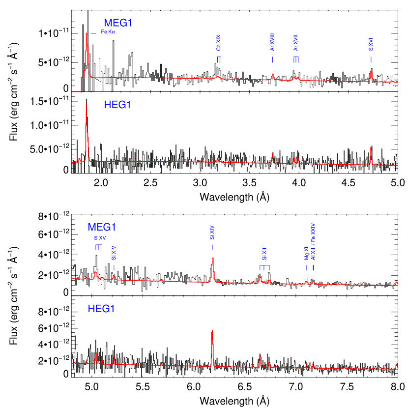
Figure 2a.— ($a$) Chandra  MEG1 and HEG1 spectra compared with the best-fit 3-$T$ model (red line) found in Tab. 2. ($b$) Same as ($a$), but for $8-14$ Å. ($c$) Same as ($a$) but for $14-26$ Å. The $17-26$ Å panels show the MEG data only.

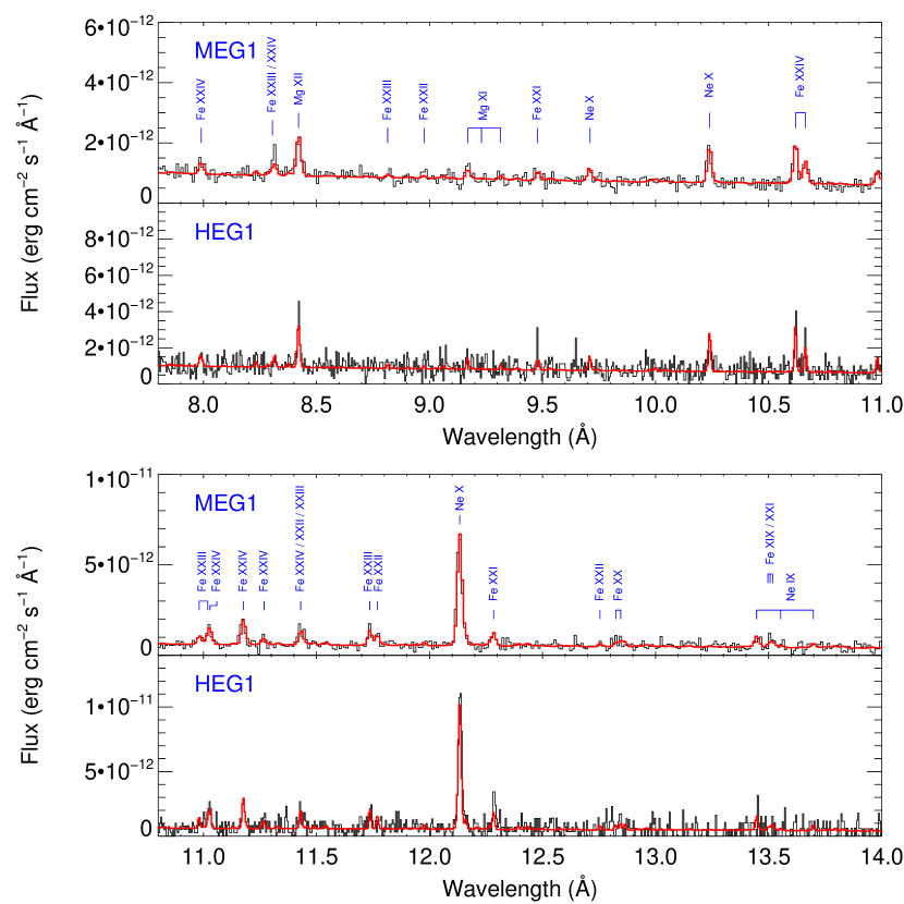
Figure 2b.—

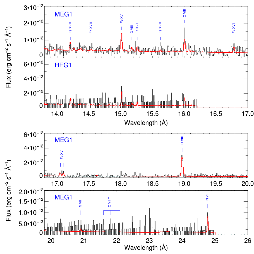
Figure 2c.—

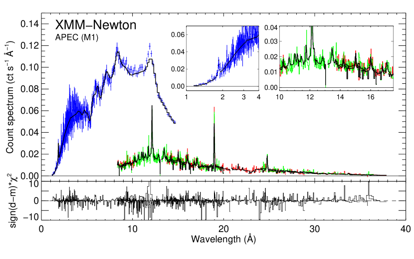
Figure 3.— XMM-Newton MOS1, RGS1, and RGS2 spectra of YY Men with the best-fit 4-$T$ model of method 1 overlaid as a thick black line. Error bars are plotted for MOS only, for clarity. Contributions to the $\chi^{2}$ (multiplied by sign[data - model]) are also plotted in the lower panel. Zoom-ins from 1 Å  to 4 Å  (logarithmic wavelength scale) and from 10 Å  to 17.5 Å  (linear wavelength scale) show the quality of the fits in the region where highly ionized Fe lines are emitted.

Figure 4.— Left: Comparison between absolute abundances derived from methods 1 and 2 with Chandra  (top panel) and XMM-Newton  (bottom panel) data. The dashed line represents a 1:1 correlation. Absolute abundances from method 2 are slightly lower with respect to those obtained from method 1 for Chandra  data (but not for XMM-Newton  data). Right: Comparison between abundance ratios derived from method 3 and methods 1 (top) and 2 (bottom) with Chandra  data. Excellent agreement is generally found.

Figure 5.— Comparison between abundances derived from methods 1 (left panels) and 2 (right panels) with XMM-Newton  and Chandra  data. The dashed line represents a 1:1 correlation. The upper panels show the absolute abundances (relative to H), and the lower panels show the abundances relative to Fe ([A/Fe] = [A/H] $-$ [Fe/H]). All abundances are relative to the solar photospheric composition (Grevesse & Sauval, 1998).

Figure 6.— Abundance ratios, [A/Fe], in YY Men’s corona as a function of the FIP. For clarity, we selected abundances from method 1, and shifted the Chandra  data points by $+0.2$ eV. The abundance ratios are relative to the solar photospheric composition (Grevesse & Sauval, 1998). The solar ratio ($\mathrm{[A/Fe]=0}$) is indicated by a dotted line.

Figure 7.— Emission measure distribution of YY Men obtained from the Chandra  and XMM-Newton  spectra for the various methods. To help comparison, we plot $\mathrm{EMD}(T)/\Delta\log T$, i.e., the EMDs per bin (see Table 2) were divided by the integration step ($0.15$ and $0.10$ dex for methods 2 and 3, respectively). For the multi-T approach (method 1), we show the EM in each component since this method has no bin width. The y-axis, therefore, reflects this distinction (left axis for methods 2 and 3, right axis for method 1). The top panel shows the EMD in a linear vertical scale to emphasize the dominant very hot plasma, whereas the lower panel uses a logarithmic vertical scale to reveal the weak, but required plasma at lower temperatures.

Figure 8.— Comparison of the EMDs obtained in this paper for YY Men (method 3, using the definition in Eq. 2) and those derived for the giants Capella, and 31 Com (Argiroffi et al., 2003; Scelsi et al., 2004). Note the much flatter EMD, the higher temperatures, and activity level of YY Men.

Figure 9.— Comparison of the results of $4$-$T$ fits of YY Men XMM-Newton  spectra with those obtained by Audard et al. (2003) for a sample of RS CVn stars of different activity levels. Also shown here is a $3$-$T$ fit of the single rapidly rotating giant 31 Com (Scelsi et al., 2004). Fits for two other FK Com-type stars (V1794 Cyg and FK Com) from Gondoin (2004) and Gondoin et al. (2002) are also shown. The lines connecting the data points of each star are an aid to the eye and have no physical meaning.

Figure 10.— Radiative cooling curve in units of erg cm³ s^-1 for $T=1-100$ MK, based on the APEC 1.3.1 database (for photon energies from 0.01 keV to 50 keV, i.e., 0.25 Å  to 1240 Å) and for best-fit XMM-Newton  abundances (M1; Tab. 2). The total radiative loss function (solid) is the sum of the continuum contribution (dash-dotted) and of the line contribution (dashed). For comparison the total radiative loss for solar abundances (Grevesse & Sauval, 1998) is shown as a dotted line.

Figure 11.— Radiative loss time, $\tau_{r}(T)=3kT/(n_{\mathrm{e}}\Lambda(T))$, in units of days derived from the radiative cooling curve, $\Lambda(T)$, in YY Men’s corona as shown in Fig. 10. Two different plasma electron densities, $n_{\mathrm{e}}=10^{9}$ and $10^{10}$ cm^-3, were used. As mentioned in Sect. 7.4, there is no evidence for higher densities in YY Men.

Figure 12.— (Top panel): Line photon luminosity distribution for Ne X Ly$\alpha$ (solid) and O VIII Ly$\alpha$ (dotted). (Bottom panel): Weighted average width distribution for the same lines (see text for details).

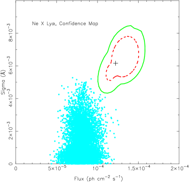
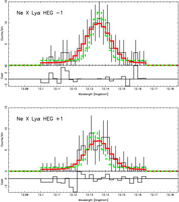
Figure 13.— (Left) Confidence map for the Ne X Ly$\alpha$ line. Confidence contours with $\Delta C=1$ and $\Delta C=2.71$ are shown in red (inner dotted contour) and green (outer solid contour), respectively. The loci of the best-fit parameters for 10,000 Monte-Carlo simulations of an emission line with an instrumental profile are shown as cyan-colored dots. (Right) HEG line profile of Ne X Ly$\alpha$ in the negative (top) and positive (bottom) order spectra. The best-fit Gaussian profile is shown as a red line (wide solid line), whereas the best-fit with the instrumental profile is shown as a green line (narrow dashed line). Residuals from the fit with a Gaussian profile are shown in sub-panels.

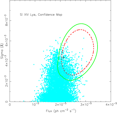
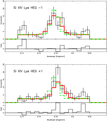
Figure 14.— Similar to Figure 13 but for Si XIV Ly$\alpha$.

References

- Argiroffi et al. (2003) Argiroffi, C., Maggio, A., & Peres, G. 2003, A&A, 404, 1033
- Arnaud (1996) Arnaud, K. A. 1996, in ASP Conf. Ser. 101, Astronomical Data Analysis Software and Systems V, ed. G. Jacoby & J. Barnes (San Francisco: ASP), 1
- Aschwanden (1999) Aschwanden, M. J. 1999, Sol. Phys., 190, 233
- Audard et al. (2001a) Audard, M., Behar, E., Güdel, M., et al. 2001a, A&A, 365, L329
- Audard et al. (2000) Audard, M., Güdel, M., Drake, J. J., & Kashyap, V. L. 2000, ApJ, 541, 396
- Audard et al. (1999) Audard, M., Güdel, M., & Guinan, E. F. 1999, ApJ, 513, L53
- Audard et al. (2001b) Audard, M., Güdel, M., & Mewe, R. 2001b, A&A, 365, L318
- Audard et al. (2003) Audard, M., Güdel, M., Sres, A., Raassen, A. J. J., & Mewe, R. 2003, A&A, 398, 1137
- Ayres et al. (1981) Ayres, T. R., Linsky, J. L., Vaiana, G. S., Golub, L., & Rosner, R. 1981, ApJ, 250, 293
- Ayres et al. (1998) Ayres, T. R., Simon, T., Stern, R. A., Drake, S. A., Wood, B. E., & Brown, A. 1998, ApJ, 496, 428
- Bedford et al. (1985) Bedford, D. K., Elliott, K. H., & Eyles, C. J. 1985, Space Science Reviews, 40, 51
- Bhatia & Doschek (1992) Bhatia, A. K. & Doschek, G. A. 1992, Atomic Data and Nuclear Data Tables, 52,
- Bidelman & MacConnell (1973) Bidelman, W. P. & MacConnell, D. J. 1973, AJ, 78, 687
- Bopp & Rucinski (1981a) Bopp, B. W. & Rucinski, S. M. 1981a, IAU Symp. 93: Fundamental Problems in the Theory of Stellar Evolution, 93, 177
- Bopp & Stencel (1981b) Bopp, B. W. & Stencel, R. E. 1981b, ApJ, 247, L131
- Brinkman et al. (2001) Brinkman, A. C., Behar, E., Güdel, M., et al. 2001, A&A, 365, L324
- Brown et al. (1998) Brown, G. V., Beiersdorfer, P., Liedahl, D. A., Widmann, K., & Kahn, S. M. 1998, ApJ, 502, 1015
- Bunton et al. (1989) Bunton, J. D., Large, M. I., Slee, O. B., Stewart, R. T., Robinson, R. D., & Thatcher, J. D. 1989, Proceedings of the Astronomical Society of Australia, 8, 127
- Cash (1979) Cash, W. 1979, ApJ, 228, 939
- Cayrel de Strobel et al. (1997) Cayrel de Strobel, G., Soubiran, C., Friel, E. D., Ralite, N., & Francois, P. 1997, A&AS, 124, 299
- Cayrel de Strobel et al. (2001) Cayrel de Strobel, G., Soubiran, C., & Ralite, N. 2001, A&A, 373, 159
- Chung et al. (2004) Chung, S. M., Drake, J. J., Kashyap, V. L., Lin, L. W., & Ratzlaff, P. W. 2004, ApJ, 606, 1184
- Collier Cameron (1982) Collier Cameron, A. 1982, MNRAS, 200, 489
- Craig & Brown (1976a) Craig, I. J. D. & Brown, J. C. 1976a, A&A, 49, 239
- Craig & Brown (1976b) ——— 1976b, Nature, 264, 340
- Cutispoto et al. (1992) Cutispoto, G., Pagano, I., & Rodono, M. 1992, A&A, 263, L3
- Doron & Behar (2002) Doron, R. & Behar, E. 2002, ApJ, 574, 518
- Drake (2003a) Drake, J. J. 2003a, Advances in Space Research, 32, 945
- Drake (2003b) Drake, J. J. 2003b, ApJ, 594, 496
- Drake & Sarna (2003c) Drake, J. J. & Sarna, M. J. 2003c, ApJ, 594, L55
- Drake et al. (2001) Drake, J. J., Brickhouse, N. S., Kashyap, V. L., et al. 2001, ApJ, 548, L81
- Drake et al. (1995) Drake, J. J., Laming, J. M., & Widing, K. G. 1995, ApJ, 443, 393
- Drake et al. (1997) ——— 1997, ApJ, 478, 403
- Drake (1996) Drake, S. A. 1996, in Proceedings of the 6th Annual October Astrophysics Conference in College Park, eds. S. S. Holt & G. Sonneborn, (San Francisco: ASP), 215
- Favata & Micela (2003) Favata, F. & Micela, G. 2003, Space Science Reviews, 108, 577
- Fekel & Balachandran (1993) Fekel, F. C., & Balachandran, S. 1993, ApJ, 403, 708
- Fekel et al. (1986) Fekel, F. C., Moffett, T. J., & Henry, G. W. 1986, ApJS, 60, 551
- Feldman (1992) Feldman, U. 1992, Physica Scripta, 46, 202
- Feldman (1996) Feldman, U. 1996, Phys. Plasmas, 3, 3203
- Feldman & Laming (2000) Feldman, U. & Laming, J. M. 2000, Phys. Scr, 61, 222
- Feldman et al. (1995) Feldman, U., Laming, J. M., & Doschek, G. A. 1995, ApJ, 451, L79
- Franciosini et al. (2001) Franciosini, E., Pallavicini, R., & Tagliaferri, G. 2001, A&A, 375, 196
- Glebocki & Stawikowski (2000) Glebocki, R. & Stawikowski, A. 2000, Acta Astronomica, 50, 509
- Gondoin (1999) Gondoin, P. 1999, A&A, 352, 217
- Gondoin (2004) Gondoin, P. 2004, A&A, 413, 1095
- Gondoin et al. (2002) Gondoin, P., Erd, C., & Lumb, D. 2002, A&A, 383, 919
- Gray (1989) Gray, D. F. 1989, ApJ, 347, 1021
- Grevesse & Sauval (1998) Grevesse, N., & Sauval, A. J. 1998, Space Science Reviews, 85, 161
- Grewing et al. (1986) Grewing, M., Bianchi, L., & Cassatella, A. 1986, A&A, 164, 31
- Güdel (1997) Güdel, M. 1997, ApJ, 480, L121
- Güdel (2004) Güdel, M. 2004, A&A Rev., 12, 71
- Güdel et al. (2001) Güdel, M., Audard, M., Briggs, K., et al. 2001, A&A, 365, L336
- Güdel et al. (2003) Güdel, M., Audard, M., Kashyap, V. L., Drake, J. J., & Guinan, E. F. 2003, ApJ, 582, 423
- Güdel et al. (2002) Güdel, M., Audard, M., Sres, A., Wehrli, R., Behar, E., Mewe, R., Raassen, A. J. J., & Magee, H. R. M. 2002, ASP Conf. Ser. 277: Stellar Coronae in the Chandra and XMM-Newton Era, 497
- Güdel et al. (1996) Güdel, M., Guinan, E. F., Skinner, S. L., & Linsky, J. L. 1996, Roentgenstrahlung from the Universe, 33
- Güdel et al. (1999) Güdel, M., Linsky, J. L., Brown, A., & Nagase, F. 1999, ApJ, 511, 405
- den Herder et al. (2001) den Herder, J. W., et al. 2001, A&A, 365, L7
- Holzwarth & Schüssler (2001) Holzwarth, V. & Schüssler, M. 2001, A&A, 377, 251
- Houck & Denicola (2000) Houck, J. C. & Denicola, L. A. 2000, ASP Conf. Ser. 216: Astronomical Data Analysis Software and Systems IX, 9, 591
- Huenemoerder (1996) Huenemoerder, D. P. 1996, ASP Conf. Ser. 109: Cool Stars, Stellar Systems, and the Sun, 9, 265
- Huenemoerder et al. (2003) Huenemoerder, D. P., Canizares, C. R., Drake, J. J., & Sanz-Forcada, J. 2003, ApJ, 595, 1131
- Huenemoerder et al. (2001) Huenemoerder, D. P., Canizares, C. R., & Schulz, N. S. 2001, ApJ, 559, 1135
- Hünsch & Schröder (1996) Hünsch, M. & Schröder, K.-P. 1996, A&A, 309, L51
- Hünsch et al. (1996) Huensch, M., Schmitt, J. H. M. M., Schröder, K.-P., & Reimers, D. 1996, A&A, 310, 801
- Hünsch et al. (1998) Hünsch, M., Schmitt, J. H. M. M., & Voges, W. 1998, A&AS, 127, 251
- Iben (1964) Iben, I. J. 1964, ApJ, 140, 1631
- Iben (1967) Iben, I. J. 1967, ARA&A, 5, 571
- Jansen et al. (2001) Jansen, F., et al. 2001, A&A, 365, L1
- Kaastra & Mewe (1995) Kaastra, J. S. & Mewe, R. 1995, A&A, 302, L13
- Kashyap & Drake (1998) Kashyap, V. L., & Drake, J. J. 1998, ApJ, 503, 450
- Kahn et al. (2001) Kahn, S. M., Leutenegger, M. A., Cottam, J., Rauw, G., Vreux, J.-M., den Boggende, A. J. F., Mewe, R., & Güdel, M. 2001, A&A, 365, L312
- Kashyap et al. (2002) Kashyap, V. L., Drake, J. J., Güdel, M., & Audard, M. 2002, ApJ, 580, 1118
- Krucker & Benz (1998) Krucker, S., & Benz, A. O. 1998, ApJ, 501, L213
- Laming (2002) Laming, J. M. 2002, ASP Conf. Ser. 277: Stellar Coronae in the Chandra and XMM-Newton Era, 25
- Laming et al. (1995) Laming, J. M., D rake, J. J., & Widing, K. G. 1995, ApJ, 443, 416
- Laming et al. (2000) Laming, J. M., Kink, I., Takacs, E., et al. 2000, ApJ, 545, L161
- Lemen et al. (1989) Lemen, J. R., Mewe, R., Schrijver, C. J., & Fludra, A. 1989, ApJ, 341, 474
- Lepson et al. (2003) Lepson, J. K., Beiersdorfer, P., Behar, E., & Kahn, S. M. 2003, ApJ, 590, 604
- Linsky (1985) Linsky, J. L. 1985, Sol. Phys., 100, 333
- Linsky & Haisch (1979) Linsky, J. L., & Haisch, B. M. 1979, ApJ, 229, L27
- Maggio et al. (1990) Maggio, A., Vaiana, G. S., Haisch, B. M., Stern, R. A., Bookbinder, J., Harnden, F. R., & Rosner, R. 1990, ApJ, 348, 253
- Mason et al. (2001) Mason, K. O., et al. 2001, A&A, 365, L36
- de Meideros & Mayor (1995) de Medeiros, J. R., & Mayor, M. 1995, A&A, 302, 745
- Mewe et al. (1982) Mewe, R., et al. 1982, ApJ, 260, 233
- Mewe et al. (2003) Mewe, R., Raassen, A. J. J., Cassinelli, J. P., van der Hucht, K. A., Miller, N. A., & Güdel, M. 2003, A&A, 398, 203
- Morrison & McCammon (1983) Morrison, R. & McCammon, D. 1983, ApJ, 270, 119
- Ness et al. (2003a) Ness, J.-U., Audard, M., Schmitt, J. H. M. M., & Güdel, M. 2003a, Advances in Space Research, 32, 937
- Ness et al. (2003b) Ness, J., Brickhouse, N. S., Drake, J. J., & Huenemoerder, D. P. 2003b, ApJ, 598, 1277
- Ness et al. (2004) Ness, J.-U., Güdel, M., Schmitt, J. H. M. M., Audard, M., & Telleschi, A. 2004, A&A, in press
- Ness et al. (2003c) Ness, J.-U., Schmitt, J. H. M. M., Audard, M., Güdel, M., & Mewe, R. 2003c, A&A, 407, 347
- Ness et al. (2002) Ness, J.-U., Schmitt, J. H. M. M., Burwitz, V., Mewe, R., Raassen, A. J. J., van der Meer, R. L. J., Predehl, P., & Brinkman, A. C. 2002, A&A, 394, 911
- Orlando et al. (2000) Orlando, S., Peres, G., & Reale, F. 2000, ApJ, 528, 524
- Osten et al. (2003) Osten, R. A., Ayres, T. R., Brown, A., Linsky, J. L., & Krishnamurthi, A. 2003, ApJ, 582, 1073
- Pallavicini et al. (1992) Pallavicini, R., Randich, S., & Giampapa, M. S. 1992, A&A, 253, 185
- Parker (1988) Parker, E. N. 1988, ApJ, 330, 474
- Parnell & Jupp (2000) Parnell, C. E., & Jupp, P. E. 2000, ApJ, 529, 554
- Peres et al. (2001) Peres, G., Orlando, S., Reale, F., & Rosner, R. 2001, ApJ, 563, 1045
- Perryman et al. (1997) Perryman, M. A. C., et al. 1997, A&A, 33, L49
- Piskunov et al. (1990) Piskunov, N. E., Tuominen, I., & Vilhu, O. 1990, A&A, 230, 363
- Porquet et al. (2001) Porquet, D., Mewe, R., Dubau, J., Raassen, A. J. J., Kaastra, J. S. 2001, A&A, 376, 1113
- Raassen et al. (2002) Raassen, A. J. J., et al. 2002, A&A, 389, 228
- Randich et al. (1993) Randich, S., Gratton, R., & Pallavicini, R. 1993, A&A, 273, 194
- Reale et al. (1993) Reale, F., Serio, S., & Peres, G. 1993, A&A, 272, 486
- Rosner et al. (1995) Rosner, R., Musielak, Z. E., Cattaneo, F., Moore, R. L., & Suess, S. T. 1995, ApJ, 442, L25
- Rosner et al. (1978) Rosner, R., Tucker, W. H., & Vaiana, G. S. 1978, ApJ, 220, 643
- Rucinski (1990) Rucinski, S. M. 1990, PASP, 102, 306
- Rutten (1987) Rutten, R. G. M. 1987, A&A, 177, 131
- Rybicki & Lightman (1979) Rybicki, G. B., & Lightman, A. P. 1979, “Radiative Processes in Astrophysics”, (Wiley: Toronto)
- Sanz et al. (2004) Sanz-Forcada, J., Favata, F., & Micela, G. 2004, A&A, 416, 281
- Scelsi et al. (2004) Scelsi, L., Maggio, A., Peres, G., & Gondoin, Ph. 2004, A&A, 413, 643
- Schaller et al. (1992) Schaller, G., Schaerer, D., Meynet, G., & Maeder, A. 1992, A&AS, 96, 269
- Schmitt & Ness (2002) Schmitt, J. H. M. M. & Ness, J.-U. 2002, A&A, 388, L13
- Schmitt & Ness (2004) Schmitt, J. H. M. M. & Ness, J.-U. 2004, A&A, 415, 1099
- Schrijver et al. (1989) Schrijver, C. J., Lemen, J. R., & Mewe, R. 1989, ApJ, 341, 484
- Schröder et al. (1998) Schröder, K.-P., Hünsch, M., & Schmitt, J. H. M. M. 1998, A&A, 335, 591
- Simon & Drake (1989) Simon, T., & Drake, S. A. 1989, ApJ, 346, 303
- Slee et al. (1987) Slee, O. B. et al. 1987, MNRAS, 227, 467
- Smith et al. (2001) Smith, R. K., Brickhouse, N. S., Liedahl, D. A., Raymond, J. C. 2001, ApJ, 556, L91
- Strüder et al. (2001) Strüder, L., et al. 2001, A&A, 365, L18
- Telleschi et al. (2004) Telleschi, A., Güdel, M., Briggs, K., Audard, M., Ness, J.-U., & Skinner, S. 2004, ApJ, submitted
- Testa et al. (2004a) Testa, P., Drake, J. J., & Peres, G. 2004a, ApJ, in press
- Testa et al. (2004b) Testa, P., Drake, J. J., Peres, G., & DeLuca, E. E. 2004b, ApJ, 609, L79
- Turner et al. (2001) Turner, M. J. L., et al. 2001, A&A, 365, L26
- van den Oord et al. (1997) van den Oord, G. H. J., Schrijver, C. J., Camphens, M., Mewe, R., & Kaastra, J. S. 1997, A&A, 326, 1090
- Vogt (1988) Vogt, S. S. 1988, in The Impact of Vey High S/N Spectroscopy on Stellar Physics, eds. G. Cayrel de Strobel, M. Spite, (Kluwer: Dordrecht), 253
- Weisskopf et al. (2002) Weisskopf, M. C., Brinkman, B., Canizares, C., Garmire, G., Murray, S., & Van Speybroeck, L. P. 2002, PASP, 114, 1
- Welty & Ramsey (1994) Welty, A. D. & Ramsey, L. W. 1994, AJ, 108, 299
- Withbroe (1975) Withbroe, G. L. 1975, Sol. Phys., 45, 301