Capture and escape in the elliptic restricted three-body problem

Abstract

Several families of irregular moons orbit the giant planets. These moons are thought to have been captured into planetocentric orbits after straying into a region in which the planet’s gravitation dominates solar perturbations (the Hill sphere). This mechanism requires a source of dissipation, such as gas-drag, in order to make capture permanent. However, capture by gas-drag requires that particles remain inside the Hill sphere long enough for dissipation to be effective. Recently we have proposed that in the circular restricted three-body problem particles may become caught up in ‘sticky’ chaotic layers which tends to prolong their sojourn within the planet’s Hill sphere thereby assisting capture. Here we show that this mechanism survives perturbations due to the ellipticity of the planet’s orbit. However, Monte Carlo simulations indicate that the planet’s ability to capture moons decreases with increasing orbital eccentricity. At the actual Jupiter’s orbital eccentricity, this effects in approximately an order of magnitude lower capture probability than estimated in the circular model. Eccentricities of planetary orbits in the Solar System are moderate but this is not necessarily the case for extrasolar planets which typically have rather eccentric orbits. Therefore, our findings suggest that these extrasolar planets are unlikely to have substantial populations of irregular moons.

1 Introduction

While the large regular moons of the giant planets follow almost circular, low inclination, prograde orbits, the aptly named irregular moons tend to do the opposite: i.e., they often have highly eccentric, high inclination orbits which may be retrograde or prograde. These moons, therefore, provide actual observational examples of the complexities of three-body dynamics. Irregular moons are thought to have been captured during the early stages of the Solar System but the detailed mechanism has not been fully elucidated. Based on a study of the circular restricted three-body problem we have recently proposed that chaos played a key role in the initial stages of capture (Astakhov et al., 2003); in this mechanism – called chaos assisted capture (CAC) – particles may initially become entangled in chaotic layers which separate directly scattering from regular (bound) regions of phase space. This temporary trapping serves to extend the lifetimes of particles within the Hill sphere thereby providing the breathing space necessary for relatively weak dissipative forces (e.g., gas-drag) to effect permanent capture. While this basic scenario may be responsible for the initial formation of families of irregular moons, other factors may affect their subsequent long term evolution including collisions; gravitational perturbations from other planets; and deviations from circularity of the planet’s orbit. Here we investigate the effect of orbital ellipticity of the planet on the capture mechanism using Monte Carlo simulations and phase space visualisations based on the Fast Lyapunov Indicator. Two representative star-planet binaries are considered: the actual Sun-Jupiter system and a hypothetical extrasolar cousin of higher orbital eccentricity. We find that the chaos-assisted capture mechanism is robust to moderate ellipticities.

Recent discoveries of numerous irregular moons at giant planets (Gladman et al., 2001; Sheppard & Jewitt, 2003; Kavelaars et al., 2004) have spurred the development of theories of their origin, which is generally thought to involve capture (Carruba et al. 2002; Yokoyama et al. 2003; Astakhov et al. 2003; Ćuk & Burns 2004; Nesvorný, Beaugé & Dones 2004; Neto et al. 2004; Kavelaars et al. 2004). These moons are considered to be primordial pieces of the Solar System captured in the amber of time. While there is, as yet, no consensus on the detailed capture mechanism of these minor bodies a number of recent studies have, nevertheless, attemped to simulate their post-capture evolution in order to explain salient aspects of their orbits. For example, several attempts have recently been made to explain the observed clustering of irregular satellites as being the result either of the breakup of a larger parent body or from catastrophic collisions between planetesimals (Nesvorný et al., 2003; Ćuk & Burns, 2004; Nesvorný et al., 2004; Kavelaars et al., 2004). These hypotheses are supported empirically by photometric surveys (Grav & Holman, 2004) which indicate that members of the clusters have similar surface colours suggesting that they may have had common progenitors. However, whatever post-capture orbital evolution occurs within the Hill sphere there has to have been an initial capture mechanism efficient enough to populate the Hill sphere with moonlets in the first place. We have recently proposed one such mechanism – chaos-assisted capture (Astakhov et al., 2003) – in which long-term, but temporary, trapping occurs in the ‘sticky’ chaotic layers lying close to Kolmogorov-Arnold-Moser (KAM, Lichtenberg & Lieberman, 1992) tori embedded within the planet’s Hill sphere. If a particle gets entangled in one of these layers then even a moderate level of dissipation (or, alternatively, slow planetary growth, Neto et al. 2004) may be sufficient to make capture permanent. It is likely that Comet-Shoemaker-Levy 9 was a recent example of an object trapped in such a chaotic zone for the best part of the last century (Chodas & Yeomans, 1996). However, the absence of a large gas cloud at Jupiter makes contemporary permanent capture of such objects by gas-drag unfeasible.

Qualitatively, in the CAC model the capture probability of a planet is largely determined by the volume of phase space (at a given energy) taken up by chaotic zones within the Hill sphere. Simulations in the circular restricted three-body problem (CRTBP) show that capture becomes less probable at higher energies because most of the phase space is directly scattering and relatively few KAM tori survive; those that do are surrounded by relatively thin chaotic layers which are less effective at trapping intruders (Astakhov et al., 2003). Factors that are not included in the CRTBP may also affect the capture mechanism, e.g., the eccentricity of the parent planet’s orbit. A more realistic extension of CAC beyond the CRTBP is, therefore, needed. As a first step we extend the model to the elliptic restricted three-body problem (ERTBP, Szebehely 1967; Llibre & Piñol 1990; Benest 2003; Pilat-Lohinger et al. 2003; Villac & Scheeres 2004; Makó & Szenkovits 2004) which allows us to model perturbations induced by deviations of the planet’s orbit from circularity. While orbital eccentricities are relatively small, although not negligible, for the giant planets of the Solar System they may be appreciable for extrasolar planets (Schneider 1999; Marcy & Butler 2000; Chiang, Fischer & Thommes 2002; Marzari & Weidenschilling 2002; Goldreich & Sari 2003; Beaugé & Michtchenko 2003; Michtchenko & Malhotra 2004). For example, compare Jupiter’s mean orbital eccentricity $e=0.04839$ to typical extrasolar planet eccentricities which lie in the range $e\sim 0.2-0.6$ (Tremaine & Zakamska, 2003). Up to now there have been more than 100 extrasolar planetary systems detected and an intriguing question is whether these massive planets might harbour moons (Barnes & O’Brien, 2002; Burns & Ćuk, 2002; Williams, 2003) which might be habitable (Williams, Kasting & Wade, 1997). As an exemplary extrasolar captor, we study a system similar in mass ratio to the idealized Sun-Jupiter binary but which follows a highly elliptic orbit. This provides a comparative estimate for the probability of capture and also suggests the ranges of energy and orbital inclination over which extrasolar irregular moons might be expected to exist.

The paper is organized as follows: Section 2 introduces the Hamiltonian for the ERTBP which, in the limit of zero ellipticity, reduces to the CRTBP. We work in a coordinate system whose origin coincides with the planet and, in actual integrations, regularise the dynamics to deal with two-body collisions (Aarseth, 2003). Because the ERTBP is explicitly time dependent it is not possible to compute conventional Poincaré surfaces of section (SOS, Lichtenberg & Lieberman, 1992) even in the planar limit so as to visualise the structure of phase space. Therefore we use the notion of a Fast Lyapunov Indicator (FLI, Froeschlé, Guzzo & Lega, 2000) to visualise the structure of phase space. Section 3 briefly discusses the CAC mechanism as applied to the CRTBP in order to facilitate comparison with the ERTBP. In particular, FLI on the surfaces of section are computed which can be compared directly with SOS in the CRTBP. This is done in Sec. 4 where Monte Carlo simulations of capture are performed. Unlike in Astakhov et al. (2003) in these simulations we do not include dissipation and, instead, focus on the distributions of particles that can be temporarily trapped in chaotic zones for very long time periods. This avoids complications associated with the best choice of dissipative force (see, e.g., Ćuk & Burns, 2004). Finally, conclusions are contained in Sec. 5.

2 Hamiltonian and methods

The CRTBP describes the dynamics of a test particle having infinitesimal mass and moving in the gravitational field of two massive bodies (the ‘primaries’ – e.g., a planet and a star) which revolve around their center of mass on a circular orbit. The equations of motion are, therefore, most naturally presented in a non-inertial coordinate system that rotates with the mean motion of the primaries (Murray & Dermott, 1999). In the rotating coordinate system the positions of the primaries are fixed. When the planet’s orbit is elliptic rather than circular a nonuniformly rotating-pulsating coordinate system is commonly used. These new coordinates have the felicitous property that, again, the positions of the primaries are fixed; however the Hamiltonian is explicitly time-dependent (Szebehely, 1967).

2.1 Hamiltonian

For our purposes it is most convenient to locate the origin at the planet (Fig. 1) because angular momentum will be measured with respect to the planet. Then, following Szebehely (1967) and Llibre & Piñol (1990), we obtain the planetocentric ERTBP Hamiltonian $H_{e}$ after introducing an isotropically pulsating length scale

$$H_{e}=E_{e}=\frac{1}{2}((p_{x}+y)^{2}+(p_{y}-x)^{2}+{p_{z}}^{2}+z^{2})-$$

$$\biggl{(}\frac{1-\mu}{\sqrt{(1+x)^{2}+y^{2}+z^{2}}}+\frac{\mu}{\sqrt{x^{2}+y^{2}+z^{2}}}+$$

$$\frac{1}{2}(x^{2}+y^{2}+z^{2})+(1-\mu)x+\frac{1}{2}(1-\mu)\biggr{)}\bigg{/}(1+e\,\cos\,f).$$ (1)

The semimajor axis of the orbit of the primaries $a_{p}$ has been scaled to unity and $e$ is the eccentricity of the planet’s orbit; $\mu=m_{1}/(m_{1}+m_{2})$, where $\mu,m_{1}$ and $m_{2}$ are the reduced mass and masses of the planet and star, respectively ($\mu=9.5359\times 10^{-4}$ for Sun-Jupiter). The true anomaly $f$, i.e. the planet’s angular position measured from the pericenter, is related to the physical time $t$ through (Szebehely, 1967)

$$\frac{df}{dt}=\frac{(1+e\,\cos\,f)^{2}}{(1-e^{2})^{3/2}}.$$ (2)

The (planet-centered) CRTBP Hamiltonian (Astakhov et al., 2003)

$$H_{c}=E_{c}=\frac{1}{2}({p_{x}}^{2}+{p_{y}}^{2}+{p_{z}}^{2})-(x\,p_{y}-y\,p_{x})-$$

$$\frac{1-\mu}{\sqrt{(1+x)^{2}+y^{2}+z^{2}}}-\frac{\mu}{\sqrt{x^{2}+y^{2}+z^{2}}}-$$

$$(1-\mu)x-\frac{1}{2}(1-\mu),$$ (3)

is recovered when $e=0$. In both cases (1) and (3), $h_{z}=x\,p_{y}-y\,p_{x}$ is the $z$-component of angular momentum ${\bf h}=(h_{x},h_{y},h_{z})$ with respect to the planet. Note that the orbital inclination $i=\arccos{h_{z}}/{|{\bf h}|}$ is invariant under isotropic pulsating rescaling from CRTBP to ERTBP. The orbit is said prograde if $i<\pi/2$ ($h_{z}>0$) and retrograde otherwise.

The Hamiltonian of the elliptic problem (1) is a periodic function of the true anomaly $f$ (which plays the role of time) and, hence, generates a non-autonomous dynamical system. Unlike the circular problem, the ERTBP does not possess an energy integral and, evidently, no such useful guiding concept as a static zero-velocity surface (Murray & Dermott, 1999) can be introduced. Furthermore, due to the extra dimension associated with the explicit time dependence, construction of the SOS and, indeed, any visual analysis of phase space seems impossible even in the planar limit.

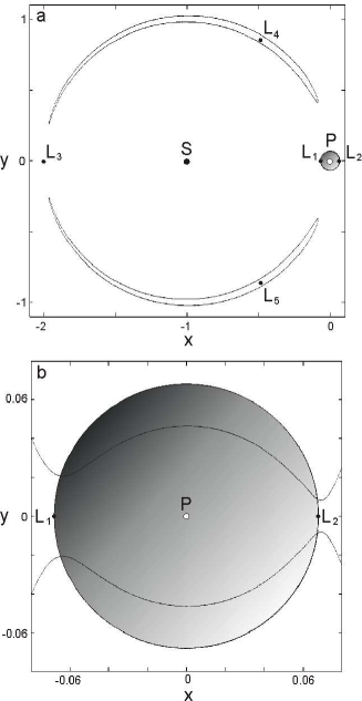
Figure 1: Level curves of the zero velocity surface at high (a) and low (b) energies in the planetocentric planar CRTBP along with the five Lagrange equillibrium points (labelled $L_{1}$ – $L_{5}$). The circle shaded grey is the Hill sphere centered on the planet (P). The star (S) is at $(-1,0)$.

2.2 Numerical methods

We have performed numerical integrations in which fluxes of particles are simulated as having passed from heliocentric orbits into the region surrounding the planet as defined by the Hill sphere. This region roughly corresponds to the region between the points labelled $L_{1}$ and $L_{2}$ in Fig. 1. In practice it is convenient to go to extended phase space by introducing an additional pair of conjugate variables – ‘coordinate’ $f$ and ‘momentum’ $p_{f}=-H$ (Lichtenberg & Lieberman, 1992) for which the new Hamiltonian becomes conservative. In our numerical simulations we have used this method in combination with Levi-Civita (in 2D) and Kustaanheimo-Stiefel (in 3D) regularising techniques (Stiefel & Scheifele, 1971; Aarseth, 2003) to avoid problems associated with two-body collisions (Nagler, 2004). Numerical integrations were done using a Bulirsch-Stoer adaptive integrator (Press et al., 1999).

Figure 2: Poincaré surfaces of section in the planar CRTPB at four energies (Jacobi constants $C_{J}=-2E_{c}$). Initial conditions were chosen randomly inside the Hill radius (here $R_{H}$ is scaled to 1) and integrated with the cut-off time $T_{cut}=36000$ years or until trajectories escaped. The SOS is the $x-y$ plane with ${p_{x}}=0,\dot{y}>0$. Points on the surface are coloured according to the sign of angular momentum $h_{z}$ as the trajectories penetrate the $x-y$ plane (black, prograde with $h_{z}>0$; grey, retrograde with $h_{z}<0$).

One approach to visualising phase space structures in systems with greater than 2 degrees-of-freedom relies on computations of short-time Lyapunov exponents (LE) over sets of initial conditions of interest (for recent developments and relevant applications see, e.g., Froeschlé et al. (2000); Sándor et al. (2001); Pilat-Lohinger et al. (2003); Cincotta, Giordano & Simó (2003); Sándor et al. (2004) and references therein, although the idea of using finite-time LE itself dates back at least to Lorenz 1965). As was demonstrated by Froeschlé et al. (2000) various dynamical regimes (including resonances) can be distinguished by monitoring time profiles of a quantity called the Fast Lyapunov Indicator. Given an $n$-dimensional continuous-time dynamical system,

$${d{\bf x}}/{dt}={\bf F}({\bf x},t),{\bf x}=(x_{1},x_{2},...,x_{n}),$$ (4)

the Fast Lyapunov Indicator is defined as (Froeschlé et al., 2000)

$$FLI({\bf x}(0),{\bf v}(0),t)=\ln|{\bf v}(t)|,$$ (5)

where v(t) is a solution of the system of variational equations (Tancredi, Sánchez & Roig, 2001)

$$\frac{d{\bf v}}{dt}=\biggl{(}\frac{\partial{\bf F}}{\partial{\bf x}}\biggr{)}{\bf v}.$$ (6)

The complementary system (6) contains spatial derivatives which only aggravate the singularities in the restricted three body problem (RTBP) and so the use of regularisation becomes even more important. For this reason, all calculations of FLI reported herein were made using regularised versions of (4) and (6).

As distinct from the largest Lyapunov characteristic exponent (Lichtenberg & Lieberman, 1992)

$$\lambda=\lim_{t\to\infty}\frac{1}{t}\ln\frac{|{\bf v}(t)|}{|{\bf v}(0)|},$$ (7)

which just tends to zero for any regular orbit, the more sensitive FLI can help discriminate between resonant and non-resonant regular orbits (Froeschlé et al., 2000). Although, in practice, detection of resonances may be tricky, since real differences in FLI for quasiperiodic and periodic orbits of the same island are not always huge.

3 Chaos assisted capture

In this section we briefly summarize the CAC mechanism described in Astakhov et al. (2003) as applied to the CRTBP. Even though the basic mechanism applies in three-dimensions, it is simpler here to outline the general scheme in terms of the planar version of the CRTBP. Fig. 1 shows the relevant zero velocity surface (ZVS, Murray & Dermott, 1999) together with the five Lagrange equilibrium points.

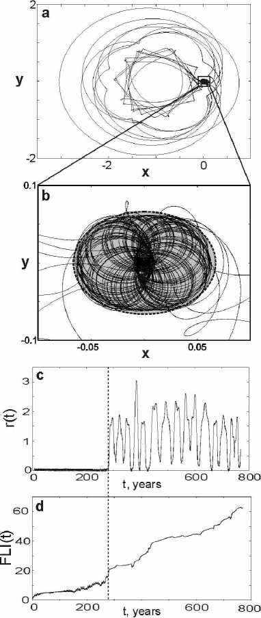
Figure 3: A paradigmatic escaping ‘sticky’ trajectory (a) in the planar Sun-Jupiter CRTBP; its multiple returns (b) to the Hill sphere (shaded grey, $R_{H}\simeq 0.068$) after heliocentric excursions; its radial distance from the planet $r=\sqrt{x^{2}+y^{2}}$ (c) and time profile of the Fast Lyapunov Indicator (d). The dotted vertical line indicates the first crossing of the Hill sphere (escape).

Level curves of the ZVS, similar to a potential energy surface (PES), serve to limit the motion in the rotating frame and so define an energetically accessible region that may intersect the Hill sphere. However, unlike a PES, because the ZVS is defined in a rotating frame, it is possible for energy maxima to be stable as is, in fact, the case for $L_{4}$ and $L_{5}$ at which points Jupiter’s Trojan asteroids are situated (Murray & Dermott, 1999). The Hill sphere (see Fig. 1) roughly occupies the region between the saddle points $L_{1}$ and $L_{2}$ which we term the ‘capture zone’ with its radius being given by $R_{H}=a_{p}/(\mu/3)^{1/3}$ where $a_{p}$ is the planet’s semimajor axis (Murray & Dermott, 1999). In the case of ERTBP the ZVS pulsates, which defines periodically time-dependent capture regions (Makó & Szenkovits, 2004). The two Lagrange saddle points $L_{1}$ and $L_{2}$ act as gateways between the Hill sphere and heliocentric orbits. A key finding of Astakhov et al. (2003) is that at energies close to (but above) the Lagrange points only prograde orbits can enter (or exit) the capture zone. At higher capture energies the distribution shifts to include both senses of $h_{z}$ until, finally, retrograde capture becomes more likely. The statistics of inclination distributions will, therefore, be expected to depend strongly on energy, i.e., how the curves of zero-velocity intersect the Hill sphere. Fig. 2 portrays the structure of phase space in the planar limit ($z=p_{z}=0$) in a series of Poincaré surfaces of section at four energies. At the lowest energy shown in Fig. 2(a) many of the prograde orbits are chaotic whereas all the retrograde orbits are regular. Because incoming orbits cannot penetrate the regular KAM tori, prograde orbits must remain prograde while retrograde orbits cannot be captured nor can already bound retrograde orbits escape. After $L_{2}$ has opened in Fig. 2(b) the chaotic ‘sea‘ of prograde orbits quickly ‘evaporates’ except for a ‘sticky’ layer of chaos which clings to the KAM tori. With increasing energy this front evolves from prograde to retrograde motion. Chaotic orbits close to the remaining tori can become trapped in almost regular orbits for very long times. In the presence of dissipation these chaotic orbits can be smoothly switched into the nearby KAM region and almost always preserve the sign of angular momentum. Thus, at low (high) energy permanent capture is almost always into prograde (retrograde) orbits.

4 Results and discussion

In this section we describe the results of our simulations in the planar ERTBP using the FLI and our Monte Carlo simulations in the spatial ERTBP.

4.1 Planar ERTBP and FLI

We are primarily interested here in obtaining a qualitative picture of the volume and structure of phase space occupied by the chaotic layer in the ERTBP as compared to the CRTBP. For this we find a good diagnostic to be $FLI(t)$ whose increase for chaotic orbits can usually be detected before, or no later than, a test particle finally escapes from the capture zone (Fig. 3). These measurements, when made over the capture region (which contains permanently bound regular trajectories even at energies well above $L_{1}$ and $L_{2}$), provide an estimate of the number of orbits that could be captured as illustrated in Fig. 4. The number of chaotic orbits inside the capture zone, detected by computing FLI, decreases with increasing ellipticity for moderate eccentricities (Fig. 4(a)) signifying that the chaotic layers get weaker and, therefore, capture is expected to become less probable than it is at $e=0$.

Ideally the problem of separating the fractions of temporarily trapped and almost immediately escaping trajectories could be better quantified by partitioning the phase space into disjoint (e.g. ‘inner’, Hill sphere, and ‘outer’, heliocentric space) regions and computing the fluxes across the barriers between them. But, given the current state of phase space transport theory, this has not yet been shown possible in practice for essentially 3D problems such as the spatial CRTBP and ERTBP Hamiltonians. Interestingly enough, despite strong theoretical grounds (Wiggins, Haller & Mezic, 1994), and exhausting attempts, efforts to describe quantitatively spatial three-body dynamics by constructing global invariant manifolds (Belbruno, 2004), that would presumably contain all possible incoming and outgoing chaotic trajectories through $L_{1}$ and $L_{2}$ saddle points, have been not quite successful in approaching the 3D problem so far. Part of the reason is that multiple escapes and recurrences of high energy trajectories to the Hill sphere (see example on Fig. 3a,b) make local manifolds near multidimensional saddles extremely difficult to use as rigorous surfaces of no return. This is even more pronounced for chaotic ionization of atomic Rydberg electrons (Brunello, Uzer & Farrelly 1997; Lee et al. 2000) which is closely related to RTBP dynamics. Recent progress in pursuit of manifolds for the spatial three-body problem is reported by Gómez et al. 2003; Villac & Scheeres 2004; Waalkens, Burbanks & Wiggins 2004.

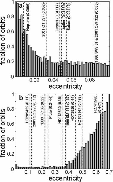
Figure 4: Fraction of chaotic orbits within the Hill sphere that have $FLI>8$ at the cut-off time $T_{cut}=200$ years in the planar Sun-Jupiter ERTBP as a function of eccentricity. The phase space was sampled randomly with initial energies, true anomalies and eccentricities taken also at random. For reference, shown in parentheses are the mean eccentricities of Jupiter, Saturn, Neptune, Uranus, Pluto, some extrasolar planetary systems (HD 209452, HD 169830, HD 73526, HD 108147, HD 74156b), and binary trans-Neptunian objects on elliptic orbits ($2001~{}QC_{297}$,$1998~{}WW_{31}$, $2001~{}QW_{322}$, $2001~{}QC_{298}$, $1999~{}TC_{36}$, $1998~{}SM_{165}$).

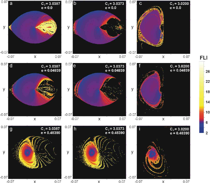
Figure 5: Colour coded Fast Lyapunov Indicator on the grid of isoenergetic (at indicated values of the Jacobi constant $C_{J}$) initial conditions taken on the $x-y$ surface of section (${p_{x}}=0,\dot{y}>0$) for the planar circular (a–c), elliptic Sun-Jupiter (d–f) and and highly elliptic extrasolar (g–i) systems. In the elliptic case, initial conditions were computed with initial $f=\pi/2$. FLI were measured at the cut-off time of $T_{cut}=200$ years. Very short-lived (scattering) trajectories that did not survive inside the Hill sphere for the cut-off time were discarded and are not shown.

To analyse the structure of phase space in ERTBP, we first computed FLI in the planar (2D) circular case ($e=0,z=p_{z}=0$), where direct comparison with surfaces of section (in the Hill limit, $\mu\ll 1$, Simó & Stuchi 2000; Astakhov et al. 2003) can be made. Figs. 5(a–c) confirm that phase space visualisation via computing short-time FLI (5) works well in the planar CRTBP, reproducing correctly all the relevant features visible in the SOS shown in Fig. 2. In particular, the chaotic layer, and its evolution with increasing energy, can be easily identified by high values of FLI (shown in yellow). Note also that FLI measurements make sense even for relatively short time integrations, and are more economical than constructing the corresponding SOS (compare cut-off times given in the Fig. 5 and Fig. 2 captions). As for the sensitivity, it is not clear how reliable the numerical distinctions (red-purple-blue) between the FLI for quasiperiodic and resonant orbits are, but this is irrelevant for our current purposes.

In the planar limit, initial conditions were generated randomly within the Hill radius on the surface of section (see Fig. 5 caption) and assuming that, initially, $f=\pi/2$ in which case the ERTBP initial conditions reduce to those of CRTBP. This guaranties that all ERTBP initial conditions are generated with identical initial energies $p_{f}(0)=-E_{e}$, and these are, in fact, true CRTBP energies $E_{c}$. The setting, thereby, allows for a direct comparison between the SOS of Fig. 2 and results obtained using the FLI. Due to the dimensionality of the ERTBP, relaxation of the above constraint, e.g. choosing the initial true anomalies at random, produced FLI maps with no distinct structure. On the contrary, consistency in initial conditions at fixed $f=\pi/2$ helps track the smooth changes from CRTBP to ERTBP.

As the planet’s orbital eccentricity is increased to reach its actual value for Jupiter, FLI maps reveal a reduction of the density of orbits within the chaotic layers (yellow paterns) visible on Fig. 5(d-f) at each of the corresponding energies shown. However, at this moderate eccentricity, the phase space structures responsible for CAC (‘sticky’ KAM tori surrounded by the chaotic layers) generally survive any deviations introduced by ellipticity. This suggests robustness of the CAC mechanism with respect to actual ellipticities of the giant planets’ orbits which lie well below $e\simeq 0.4$ (see Fig. 4). We further confirm this by direct Monte Carlo simulations of capture probability (Sec. 4.2) which reveal that CAC indeed survives weak ellipticity in the RTBP. An important implication for future studies can be drawn by noticing that the heliocentric orbits of Pluto (with Charon) as well as of some recently discovered binary trans-Neptunian objects are quite eccentric (see examples on Fig. 4), but not to the extent characteristic of extrasolars (although the relative orbit of the binary partners as distinct from the heliocentric orbit of the combine can be very eccentric). These binary objects can be viewed in the framework of the Hill approximation too, so the weakly elliptic chaos-assisted mutual capture, probably stabilized by the fast exchange of energy and angular momentum with a fourth body, may have been involved in early stages of their formation (Goldreich, Lithwick & Sari 2002; Astakhov et al. 2003; Funato et al. 2004).

The picture at much higher eccentricities evolves towards significant distorsions of the phase space stuctures as visualised by FLI. In Fig. 5(g–i) the KAM tori (red–blue islands) shrink, giving way to regions of scattering and chaotic orbits with short (200 years in this example) residence times inside the Hill sphere. These short-lived trajectories are the main contributions to the rapidly increasing number of chaotic orbits observed in Fig. 4 for $e>0.4$. This does not mean, however, that capture will necessarily be enhanced, because a high density of strongly chaotic orbits does not correlate with the number of very long-lived trajectories trapped close to KAM tori.

On the other hand, Lyapunov exponents computed for individual trajectories cannot serve as a predictor of global stability, i.e. as an indicator of whether an orbit will stay long enough in a bound region, or if it escapes quickly. This aspect in computing Lyapunov exponents for escaping (captured) trajectories concerns the notion of ‘stable chaos’ (Milani & Nobili, 1992). This term was coined to refer to chaotic motions that are locally hyperbolic, but demonstrate macroscopic long-term stability, so that the Lyapunov time $T_{L}$ (the inverse of the largest Lyapunov exponent (7)) is substantially less than the ’event’ time $T_{E}$, e.g. the time for a trajectory to leave a certain region. However, there are indications of a possible simple linear correlation between $T_{E}$ and $T_{L}$ as shown in Lecar, Franklin & Murison (1992), which suggests that knowledge of the Lyapunov time could allow one to predict an ’event’ time. Concerning the residence (escape) time near the planet, simulations in the planar CRTBP, however, show that such a correlation with the Lyapunov time does not exist (Fig. 6, see also discussion by Morbidelli & Froeschlé 1996 and Varvoglis & Anastasiadis 1996). Among the randomly chosen escaping chaotic trajectories originating in the Hill sphere, there are many very long-lived examples that have diverse, even quite small, Lyapunov times. This means that local (microscopic) instabilities in the chaotic layer alone cannot explain the distributions of survival probability. Rather, as was pointed out by Tsiganis, Anastasiadis & Varvoglis (2000), long-term trapping with short $T_{L}$ near ‘sticky’ KAM structures can be attributed to the existence of phase space quasi-barriers and approximate integrals of motion. In the case of RTBP, these are the phase space structures around the saddle points at $L_{1}$ and $L_{2}$ and the $z$-component of angular momentum with respect to the planet, respectively. In 3D, the latter is approximately conserved (Contopolous, 1965) for long-lived chaotic orbits which explains the unexpected strong correlation between initial and final inclinations of captured particles (‘inclination memory’, Astakhov et al., 2003).

4.2 Monte Carlo simulations in the spatial ERTBP

We simulated capture statistics in the spatial (three-dimensional) ERTBP by integrating isotropic fluxes of test particles that bombard the capture zone producing equal probabilities of initial conditions. Initial conditions were generated as follows: the particle’s position vector was chosen uniformly and randomly on the surface of the Hill sphere. Velocities were also chosen uniformly and randomly in accordance with the value of the CRTBP energy $E_{c}$. In turn, the starting energy (Jacobi constant $C_{J}=-2E_{c}$) was chosen uniformly random between its minimum possible value (as defined by the energy of $L_{1}$ when $f=\pi/2$) and its highest value (determined empirically such that above it the capture probability was essentially zero.) Then, by randomizing the initial true anomaly $f$ we model equal chances for a test particle to have any phase with respect to the mutual revolution of the primaries. The trajectories were integrated until one of the following occurred: the particle exited the Hill sphere; it penetrated a sphere, centred on the planet, of a given radius (see Fig. 7 caption); it survived for a predetermined cut-off time.

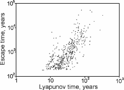
Figure 6: Escape time versus Lyapunov time for 2D CRTBP chaotic trajectories with initial conditions chosen randomly inside the Hill sphere. Escape was defined as the first crossing of the Hill sphere.

Choosing particles on the Hill sphere, where the motion is chaotic or scattering, minimizes (although does not eliminate) the risk of accidentally starting orbits inside impenetrable KAM regions (Neto et al., 2004). Although permanently bound, these orbits could never actually have been captured because KAM regions cannot be penetrated at all in 2D and only exponentially slowly in 3D. It is only in the chaotic layer between scattering and stability that capture can happen. An initial swarm of incoming particles produces broad distribution of survivors with different residence times inside the Hill sphere. We monitored its dynamics up to certain cut-off times (of the order of several thousand years) to find those long-lived chaotic orbits that may have been vulnerable to capture by a relatively weak dissipative force such as gas drag. Only these orbits, in the CAC model, could be the precursors to the currently observed distributions of irregular satellites. In a statistical sense, any short-time flybys are unlikely to have contributed to the primordial population of potential moons. Also, since the Sun-Jupiter system was chosen as an example, we eliminated test particles that penetrated the inner region of the Hill sphere occupied by Jupiter’s most influencial regular moon Callisto. The massive regular moons may have acted as a source of strong perturbation removing some temporarily captured moonlets following prograde orbits. This provides a possible reason for the observed prograde-poor distribution of jovian irregulars (Astakhov et al., 2003).

Fig. 7 shows the results of these simulations. The capture probability density is plotted on the plane of initial and final inclinations. Unlike other properties, e.g., energy, inclination can be defined consistently in both the CRTBP and the ERTBP ($e=0$ and $e>0$ in isotropically pulsating coordinates). As the distributions in Fig.7 confirm, inclination is approximately conserved during temporary capture in the ERTBP, so that the RTBP energy/inclination dependent CAC mechanism survives additional perturbations caused by deviations of the planet’s orbit from circularity. This is clearly seen upon comparing Fig.7 (a) and (b). The latter shows the capture probability for the Sun-Jupiter system with its actual eccentricity being used. We also verified by similar Monte Carlo runs that the basic energy–inclination correlation discussed in Sec. 3 remains valid in the 3D ERTBP. We note, however, that since the energy is not a conserved quantity in the elliptic problem, a better representation of results is given in terms of inclinations.

The most prominent effect observed in the ERTPB compared to the circular case is the overall decrease of capture probability as eccentricity increases. Simulations indicate that, given the same time scale, the actual ellipticity of Jupiter’s orbit accounts for approximately an order of magnitude lower capture probability than predicted by the circular model, while the relative number of progrades versus retrogrades remains unaffected.

Capture by typical extrasolar planets will be expected to become even more suppressed due to the wildly eccentric nature of these, essentially ERTBP, star–planet systems. To test this we used an eccentricity $e=0.4839$ which is ten times greater than that of Jupiter’s orbit but quite similar to what has been estimated, for instance, for several already detected extrasolars (the values of $e$ are given in parentheses): HD 108147 (0.498), HD 168443b (0.53), HD 82943c (0.54), HD 142415 (0.5), HD 4203 (0.46), HD 210277 (0.46), HD 147513 (0.52), HD 190228 (0.5), HD 50554 (0.5), HD 33636 (0.53). For consistency, we left unchanged all of the other parameters and environmental factors (including Callisto whose hypothetical extrasolar analogs may well exist around exo-Jupiters) exactly as they were used in the simulations for Sun-Jupiter. Fig.7(c) indicates that, due to the ellipticity of the orbits and assuming similar time scales and other conditions, capture by extrasolar planets may be as much as aproximately ten times less efficient than it could be by the giant planets of our system.

The relatively low capture probability, predicted in ERTBP, adds to other destructive mechanisms possibly operating on as yet undiscovered irregular satellites of extrasolar planets. The loss of satellites through Yarkovsky (Burns & Ćuk, 2002) or tidal (Barnes & O’Brien, 2002) effects may also diminish the possibility for highly elliptic extrasolar captors to marshal large populations of irregular moons. On the other hand, exo-planets with masses from one-half to four times Jupiter’s mass on low eccentricity orbits ($e<0.02$) may be considered candidates for having irregular satellites. These may include, e.g., already known extrasolars such as HD 179949, 55 Cnc b, HD 169830c, HD 187123, Tau Boo, HD 75289, 51 Peg, Ups And b, HD 195019.

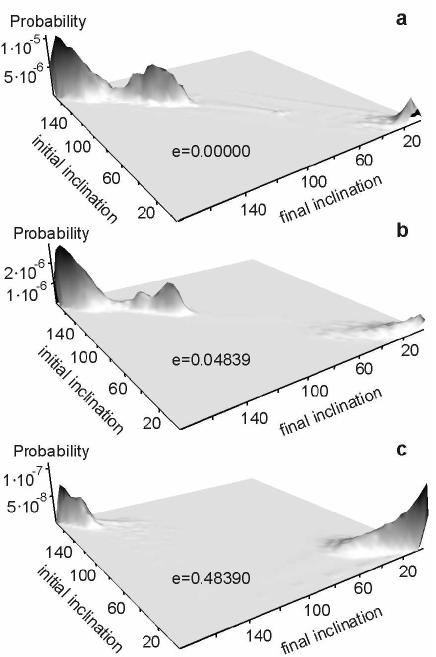
Figure 7: Capture probability (the density of survivors normalized by the number of trajectories in the incoming fluxes) as a function of initial and final inclinations in spatial circular (a), elliptic Sun-Jupiter (b) and exemplary elliptic extrasolar (c) RTBP systems. The values of eccentricity $e$ are shown. Chaotic trajectories with random energies ($C_{J}\in[2.995,{C_{J}}^{(L_{1})}]$), true anomalies ($f\in[0,2\pi]$), velocities and coordinates (on the Hill sphere with the radius $R_{H}\simeq 0.068$) were integrated until they either escaped from the sphere or crossed Callisto’s orbit at $r=2.42\times 10^{-3}$ (Jupiter’s orbital semimajor axis $a_{p}=1$). Each of the distrubutions was drawn from orbital elements of $N\simeq 20000$ long-lived chaotic orbits that entered and survived within the Hill sphere for $T_{cut}=20000$ years. Incoming fluxes consisted of $3\times 10^{7}$ (a), $1.6\times 10^{8}$ (b), $4.6\times 10^{9}$ (c) particles.

5 Conclusions

The complexity of many-body systems evidently goes far beyond that of the simplest non-trivial case, the three-body problem. However, when considered on a hierarchical level, interactions between gravitional centers can often be decomposed to relatively low degree-of-freedom subsystems for which analysis from a dynamical systems point of view becomes possible. In the problem described here, the existence of ’sticky’ volumes of phase space where regular regions are surrounded by chaotic layers explains why several bodies may become temporarily (but for rather long time periods) trapped by mutual chaos-assisted capture. These quasi-stable configurations can subsequently be stabilised (or destroyed) on much longer time scales by various forces (dissipative or not). Here we have considered the effect introduced by a slow (compared to time-scales of motion in the chaotic layer) periodic parametric time dependence in the three-body problem. Our simulations show that chaos-assisted capture applies and is, in fact, only slightly perturbed in cases when the primaries move on an elliptic orbit. It is expected to be of significant interest (e.g. in applications to essentially many-particle systems such as star clusters and the asteroid belt) to consider chaos-assisted capture at the next hierarchical level, i.e. when the primary two-body configuration is not restricted to a regular orbit, which may be the case in three-body encounters of comparably sized objects.

References

- Aarseth (2003) Aarseth S. J., 2003, Gravitational N-body Simulations: Tools and Algorithms. Cambridge Univ. Press, Cambridge
- Astakhov et al. (2003) Astakhov S. A., Burbanks A. D., Wiggins S., Farrelly D., 2003, Nature, 423, 264
- Barnes & O’Brien (2002) Barnes J. W., O’Brien D. P., 2002, ApJ, 575, 1087
- Beaugé & Michtchenko (2003) Beaugé C., Michtchenko T. A., 2003, MNRAS, 341, 760.
- Benest (2003) Benest D., 2003, A&A, 400, 1103
- Belbruno (2004) Belbruno E., 2004, Capture Dynamics and Chaotic Motions in Celestial Mechanics. Princeton Univ. Press, Princeton and Oxford
- Brunello et al. (1997) Brunello A. F., Uzer T., Farrelly D., 1997, Phys. Rev. A, 55, 3730
- Burns & Ćuk (2002) Burns J. A., Ćuk M., 2002, BAAS, 34, DPS 34th Meeting, abstr. No. 42.01
- Carruba et al. (2002) Carruba V., Burns J. A., Nicholson P. D., Gladman B. J., 2002, Icarus, 158, 434
- Chiang et al. (2002) Chiang E. I., Fischer D., Thommes E., 2002, ApJ, 564, L105
- Chodas & Yeomans (1996) Chodas P. W., Yeomans D. K., 1996, in Knoll K. S., Weaver H. A., Feldman P. D., ed., The collision of Comet Shoemaker-Levy 9 and Jupiter. Cambridge Univ. Press, Cambridge
- Cincotta et al. (2003) Cincotta P. M., Giordano C. M., Simó C., 2003, Physica D, 182, 157
- Contopolous (1965) Contopoulos G., 1965, ApJ, 142, 802
- Ćuk & Burns (2004) Ćuk M., Burns J. A., 2004, Icarus, 167, 369
- Froeschlé et al. (2000) Froeschlé C., Guzzo M., Lega E., 2000, Science, 289, 2108
- Funato et al. (2004) Funato Y., Makino J., Hut P., Kokubo E., Kinoshita D., 2004, Nature, 427, 518
- Gladman et al. (2001) Gladman B. et al., 2001, Nature, 412, 163
- Goldreich & Sari (2003) Goldreich P., Sari R., 2003, ApJ, 585, 1024
- Goldreich et al. (2002) Goldreich P., Lithwick Y., Sari R., 2002, Nature, 420, 643
- Gómez et al. (2003) Gómez G., Koon W. S., Lo M. W., Marsden J. E., Masdemont J., Ross S. D., 2004, Nonlinearity, 17, 1571
- Grav & Holman (2004) Grav T., Holman M. J., 2004, ApJ, 605, L141
- Kavelaars et al. (2004) Kavelaars J. J. et al., 2004, Icarus, 169, 474
- Lecar et al. (1992) Lecar M., Franklin F., Murison M., 1992, AJ, 104, 1230
- Lee et al. (2000) Lee E., Brunello A. F., Cerjan C., Uzer T., Farrelly D., 2000, in Yeazell J., Uzer T., ed., The Physics and Chemistry of Wave Packets, Wiley, NY, p. 95
- Lichtenberg & Lieberman (1992) Lichtenberg A. J., Lieberman M. A., 1992, Regular and Chaotic Dynamics, 2nd edn. Springer-Verlag, NY
- Llibre & Piñol (1990) Llibre J., Piñol J., 1990, Celest. Mech. Dynam. Astronom., 48, 319
- Lorenz (1965) Lorenz E. N., 1965, Tellus, 17, 321
- Makó & Szenkovits (2004) Makó Z., Szenkovits F., 2004, Celest. Mech. Dynam. Astronom., in press
- Marcy & Butler (2000) Marcy G. W., Butler R. P., 2000, PASP, 112, 137
- Marzari & Weidenschilling (2002) Marzari F., Weidenschilling S. J., 2002, Icarus, 156, 570
- Michtchenko & Malhotra (2004) Michtchenko T. A., Malhotra R., 2004, Icarus, 168, 237
- Milani & Nobili (1992) Milani A., Nobili A. M., 1992, Nature, 357, 569
- Morbidelli & Froeschlé (1996) Morbidelli A., Froeschlé C., 1996, Celest. Mech. Dynam. Astronom., 63, 227
- Murray & Dermott (1999) Murray C. D., Dermott S. F., 1999, Solar System Dynamics. Cambridge Univ. Press, Cambridge
- Nagler (2004) Nagler J., 2004, Phys. Rev. E, 69, 066218
- Nesvorný et al. (2003) Nesvorný D., Alvarellos J. L. A., Dones L., Levison H. F., 2003, AJ, 126, 398
- Nesvorný et al. (2004) Nesvorný D., Beaugé C., Dones L., 2004, AJ, 127, 1768
- Neto et al. (2004) Neto E. V., Winter O. C., Yokoyama T., 2004, A&A, 414, 727
- Pilat-Lohinger et al. (2003) Pilat-Lohinger E., Funk B., Dvorak R., 2003, A&A, 400, 1085
- Press et al. (1999) Press W. H., Teukolsky S. A., Vetterling W. T., Flannery B. P., 1999, Numerical Recipes in C, 2nd edn. Cambridge Univ. Press, Cambridge
- Sándor et al. (2001) Sándor Z., Balla R., Téger F., Érdi B., 2001, Celest. Mech. Dynam. Astronom., 79, 29
- Sándor et al. (2004) Sándor Z., Érdi B., Széll A., Funk B., 2004, Celest. Mech. Dynam. Astronom., in press
- Schneider (1999) Schneider J., 1999, CR Acad. Sci. II B, 327, 621
- Sheppard & Jewitt (2003) Sheppard S., Jewitt D., 2003, Nature, 423, 261
- Simó & Stuchi (2000) Simó C., Stuchi T. J., 2000, Physica D, 140, 1
- Stiefel & Scheifele (1971) Stiefel E. L., Scheifele G., 1971, Linear and Regular Celestial Mechanics: Perturbed Two-Body Motion, Numerical Methods, Canonical Theory. Springer-Verlag, New York
- Szebehely (1967) Szebehely V., 1967, Theory of Orbits: the Restricted Problem of Three Bodies. Acad. Press, NY and London
- Tancredi et al. (2001) Tancredi G., Sánchez A., Roig F., 2001, AJ, 121, 1171
- Tsiganis et al. (2000) Tsiganis K., Anastasiadis A., Varvoglis H., 2000, Chaos, solitons and fractals, 11, 2281
- Tremaine & Zakamska (2003) Tremaine S., Zakamska N. L., 2003, preprint (astro-ph/0312045)
- Varvoglis & Anastasiadis (1996) Varvoglis H., Anastasiadis A., 1996, AJ, 111, 1718
- Villac & Scheeres (2004) Villac B. F., Scheeres D. J., 2004, A simple algorithm to compute hyperbolic invariant manifolds near and , 14th AAS/AIAA Space Flight Mechanics Meeting, February 2004, Maui, Hawaii
- Waalkens et al. (2004) Waalkens H., Burbanks A., Wiggins S., 2004, J. Phys. A: Math. Gen, 37, L257
- Wiggins (1994) Wiggins S., Haller G., Mezic I., 1994, Normally Hyperbolic Invariant Manifolds in Dynamical Systems (Applied Mathematical Sciences, Vol 105). Springer-Verlag, NY
- Williams (2003) Williams D. M., 2003, BAAS, 35, DPS 35th Meeting, abstr. No. 27.10
- Williams et al. (1997) Williams D. M., Kasting J. F., Wade R. A., 1997, Nature, 385, 234
- Yokoyama et al. (2003) Yokoyama T., Santos M. T., Cardin G., Winter O. C., 2003, A&A, 401, 763