Downscattering due to Wind Outflows in Compact X-ray Sources: Theory and Interpretation

Abstract

A number of recent lines of evidence point towards the presence of hot, out-flowing plasma from the central regions of compact Galactic and extragalactic X-ray sources. Additionally, it has long been noted that many of these sources exhibit an “excess” continuum component, above $\sim 10$ keV, usually attributed to Compton Reflection from a static medium. Motivated by these facts, as well as by recent observational constraints on the Compton reflection models – specifically apparently discrepant variability timescales for line and continuum components in some cases – we consider possible effects of out-flowing plasma on the high-energy continuum spectra of accretion powered compact objects. We present a general formulation for photon downscattering diffusion which includes recoil and Comptonization effects due to divergence of the flow. We then develop an analytical theory for the spectral formation in such systems that allows us to derive formulae for the emergent spectrum. Finally we perform the analytical model fitting on several Galactic X-ray binaries. Objects which have been modeled with high-covering-fraction Compton reflectors, such as GS1353-64 are included in our analysis. In addition, Cyg X-3, is which is widely believed to be characterized by dense circumstellar winds with temperature of order $10^{6}$ K, provides an interesting test case. Data from INTEGRAL and RXTE covering the $\sim 3-300$ keV range are used in our analysis. We further consider the possibility that the widely noted distortion of the power-law continuum above 10 keV may in some cases be explained by these spectral softening effects.

1 INTRODUCTION

Recent observational and theoretical evidence suggest that accretion-powered X-ray sources, of both the Galactic and extragalactic variety, may exhibit outflowing plasma, i.e. winds, emanating from a compact region near the central source (e.g. Elvis 2003; Arav 2003; Brandt & Schulz 2000; Proga & Kallman 2002). Comptonization effects in those putative outflows are likely to alter the intrinsic continuum spectra of accretion powered compact objects. The basic idea is that electron scattering of photons from a central source entering the expanding outflow experience a decrease in energy (downscattering). The magnitude of this decrease is of first order in $v/c$ and in $E/m_{e}c^{2}$ where $v$ is the outflow speed, c is the speed of light, $E$ is the initial photon energy, and $m_{e}$ is the electron rest mass.

The basic idea is depicted in Figure 1. There present a simple explanation of the diverging flow effect on the photon propagation through the medium. A photon emitted outwards near inner boundary and then scattered at a certain point by an electron moving with velocity ${\bf v}_{1}$, is received by an electron moving with velocity ${\bf v}_{2}$ as shown with frequency $\nu_{2}=\nu_{1}\left[1+\left({\bf v}_{1}-{\bf v}_{2}\right)\cdot{\bf n}/c\right]$ where ${\bf n}$ is a unit vector along the path of the photon at the scattering point. In a diverging flow $\left({\bf v}_{1}-{\bf v}_{2}\right)\cdot{\bf n}/c<0$ and photons are successively redshifted, until scattered to an observer at infinity. The color of photon path (in Figure 1) indicates the frequency shift in the rest frame of the receiver (electron or the Earth observer). On the other hand, referring to the right-hand side of Figure 1, in a converging flow $\left({\bf v}_{1}-{\bf v}_{2}\right)\cdot{\bf n}/c>0$ and photons are blueshifted.

The classical Compton (recoil) effect $<\Delta E>/E\sim-E/m_{e}c^{2}$ has been well understood for a long time. Basko, Sunyaev & Titarchuk (1974), hereafter BST74 first studied the downscattering effects in the interaction of X-ray radiation of the central source with the relatively cold atmosphere of the optical companion in a binary system. They predicted the shape of the X-ray reflection spectrum of the companion and applied these results to the Her X-1 system. X-ray observations of Her X-1 by a number of groups (e.g. Sheffer et al. 1992, Still et al. 2000 and etc.) confirmed this prediction. In particular, the numerical calculations by BST74 demonstrated that the reflection of the bremsstrahlung spectrum distorted the high-energy continuum above 10 keV producing the characteristic continuum excess feature, or “bump”, in the $>10$ keV spectrum. This feature was also identified by Sunyaev & Titarchuk (1980), hereafter ST80, who found that the transmitted, downscattered spectrum is formed as a result of the reprocessing of X-ray radiation from the central source in an ambient spherical cloud. From these facts one can conclude that this distortion of the continuum is not an intrinsic property of the particular space photon distribution, but it is rather a result of effective downscattering (in terms of the mean number of scattering and the energy loss per scattering) X-ray photons diffusing through the intervening medium.

In this paper we show that this is precisely the case. We formulate the problem of the photon diffusion in generic terms and demonstrate a specific solution for bulk motion where effects of a recoil and divergence of the flow are taken into account. The emergent spectrum as an outcome of this solution has all these aforementioned features of the downscattering.

The details of the radiative transfer problem taking into account downscattering effects (recoil and Doppler effect in the divergent flow) and its solution are given in §2. In section 3, we apply our model to observational data for several Galactic X-ray binaries. We attempt to demonstrate the Compton downscattering effects in relatively cold outflows for which temperature is of order $10^{6}$ K and disk atmospheres which are necessary constituents of X-ray sources. For example, Cygnus X-3 is believed to be characterized by dense circum-stellar (or circum-disk) winds, provides an interesting test case. A number of additional sources, which have been noted in the literature to exhibit evidence for strong“Compton reflection”, e.g. GS1353-64 and GX339-4, have also been included in our analysis. We consider the possibility that this well documented distortion of the power-law continuum above 10 keV, may in some cases be due to downscattering from out-flowing plasma rather than from a static reflecting media. We further speculate that this could possibly apply to extra-galactic (i.e. AGN) as well as Galactic accretion objects (§4), although we do not present any analysis of AGN here. A summary and conclusions follow in §5.

2 RADIATIVE TRANSFER IN A BULK OUTFLOW

2.1 The Basic Downscattering Problem

The problem of photon propagation in a fluid in bulk motion has been studied in detail in a number of papers [see e.g. Blandford & Payne (1981), hereafter BP81; Payne & Blandford (1981), hereafter PB81; Nobili, Turolla & Zampieri (1993); Titarchuk, Mastichiadis & Kylafis (1997); Titarchuk, Kazanas & Becker (2003, hereafter TKB03); Laurent & Titarchuk (1999), (2001), (2004, hereafter LT04]. In particular, TKB03 present a general formulation and a solution of the spectral formation in the diverging outflow. They demonstrated that the resulting spectrum can be formed as a convolution of energy and space diffusion solutions. The spread function, given by a Green’s function formulation, applied to a monochromatic injection yields a redshift-skewed line which is a power law at low energies. Furthermore, Monte-Carlo simulations show that the line width has a strong dependence on $v/c$, optical depth $\tau$ and the energy of the monochromatic line $E_{0}$ only when the flow temperature $kT_{e}<1$ keV (LT04). TKB03 and LT04 also establish that the shape of the spectral line should be closely related to the photon source distribution in the flow. Comparison of the theoretical spectra with data show that observed red-skewed lines are formed as a result of transmission of the X-ray radiation through outflows of moderate Thomson optical depth ($\tau_{0}{{}_{>}\atop{}^{\sim}}1$).

To apply these Radiative Transfer results to observational data, we have developed a generic analytical formulation which leads to a simple analytic expression for modification of the emergent spectrum due to recoil and velocity divergence effects in the flow. For the recoil effect, we extend the results of ST80 who show that the downscattering feature, or ”bump”, can appear superposed on power-law spectra with energy spectral indices $\alpha<1$ as a result of photon diffusion through a static cloud. From ST80 and calculations presented here, one might conclude such bumps are not a necessarily a feature of disk reflection, but could instead be a generic feature of the photon reprocessing in a relatively cool, ambient plasma characterized by temperatures of order $10^{6}$ K.

2.2 Main Equations and Solution of Downscattering Problem

Let $N(r)=N_{0}(r_{0}/r)^{b}$ be the radial number density profile of an outflow and let its radial outward speed be

$$v_{b}/c=(\dot{M}_{out}/4\pi cm_{p}N_{0}r_{0}^{2})(r_{0}/r)^{2-b}=(v_{0}/c)(r_{0}/r)^{2-b}$$ (1)

obtained from mass conservation in a spherical geometry (here $\dot{M}_{out}=4\pi r^{2}v_{b}m_{p}N$ and $m_{p}$ is the proton mass). The Thomson optical depth of the flow from some radius r to infinity is given by

$$\tau=\int_{r}^{\infty}N_{e}(r)\sigma_{\rm T}~{}dr=\sigma_{\rm T}N_{0}r_{0}(r_{0}/r)^{b-1}/(b-1),$$ (2)

where $N_{e}(r)=N(r)$ is the electron density, $\sigma_{\rm T}$ is the Thomson cross section, $r_{0}$ is a radius at the base of the outflow. Because our final results are independent of the velocity and density profiles below for simplicity of presentation we use $b=2$ (a constant velocity outflow). In this case $\tau_{0}=\tau(r_{0})=\sigma_{\rm T}N_{0}r_{0}$.

The transfer of radiation within the flow in space and energy is governed by the photon kinetic equation (BP81, Eq. 18) for the photon occupation number $n(r,\nu)$, which in steady state reads

$$-\frac{{\bf v_{b}}/c}{\kappa}\cdot\nabla n+\frac{1}{3\kappa}\nabla\cdot(\frac{1}{\kappa}\nabla n)+\frac{1}{3}\frac{\nabla\cdot{({\bf v_{b}}/c})}{\kappa}\,z\frac{\partial n}{\partial z}+\frac{1}{z^{2}}\frac{\partial(z^{4}n)}{\partial z}=-{j}(r,\nu),$$ (3)

where $z=h\nu/m_{e}c^{2}$ is the dimensionless photon energy, $\kappa=N_{e}(r)\sigma_{\rm T}$ is the inverse of the scattering mean free path, ${\bf v_{b}}=v_{b}{\bf e_{r}}$, is the flow velocity, ${\bf e_{r}}$ is the radial unit vector and $j(r,\nu)$ is the photon source term.

The spectral flux $F(r,\nu)$ (PB81) is given in terms of $n(r,\nu)$ by

$$F(r,\nu)=-\frac{1}{3\kappa(r)}\nabla n-\frac{1}{3}v_{b}\,\nu\frac{\partial n}{\partial\nu},$$ (4)

and must satisfy the following boundary conditions: (a) Conservation of the frequency integrated flux over the outer boundary, namely

$$L^{(1)}_{r}n=\int F(r,\nu)d\nu\propto r^{-2}~{}~{}~{}{\rm as}~{}~{}{\rm r\rightarrow\infty}.$$ (5)

(b) In terms of the specific intensity of the radiation, the second inner boundary condition specifies that the escaping radiation from the inner boundary be equal to the radiation entering the wind shell through the inner boundary (see Fig. 1 for the wind geometry). We neglect here the possible absorption of the radiation at the central source (black hole). Thus the occupation number should satisfy some kind of the reflection condition at the inner boundary $r=r_{0}$. Namely the photon flux at the inner boundary is zero (all photons scattered in the outflow shell and escape through the inner boundary subsequently return).

$$L_{r}^{(2)}n(r_{0})=0.$$ (6)

In this formulation of the problem the number of photons emitted in the wind shell equals to that escaped to the Earth observer (i.e. the photon number is conserved). This can be proven using Eqs. (3), (4-5). Consequently, if the high energy photons lose their energy in the way out but the number of photons is conserved it has to be the accumulation of the photons at a particular lower energy band. This accumulation effect was previously noted by ST80 for the case when the photon energy loss (downscattering) was determined by the recoil effect only (see Fig. 10 in there). In section 2.3 we demonstrate this accumulation effect when the recoil and flow divergence dowscattering effects are taken into account.

It is worth noting that in TKB03 the goal was to demonstrate the pure effect of the flow divergence on a spectral line as a result of multiple scatterings with the plasma free electrons. They thus omitted the recoil term in the left hand side of equation (3). They were also interested to applying their solution to the spectral formation of iron lines for which photon energies are about 6.4 keV and lower. For such energies the recoil effect can be safely neglected (see ST80). On the other hand if one is interested in the modification of continuum spectrum at energies higher than 10 keV by multiple downscattering events in the “cold” medium this effect must be taken into account. Below we show how one can generalize the TKB03 solution including the recoil term in the radiative transfer equation. We apply a particular method for the separation of variables suggested in Titarchuk (1994), hereafter T94, and successfully used in TKB03, to obtain our solution.

In order to further proceed with the solution derivation we should note that Laurent and Titarchuk (2004) find that the coefficient in the diverging term of equation (3) $\tilde{\varepsilon}=\nabla\cdot({\bf v_{b}}/c)/\kappa$ can be replaced by a constant $\tilde{\varepsilon}$. Strictly speaking $\tilde{\varepsilon}$ is a function of $r$ and consequently of $\tau$, namely $\tilde{\varepsilon}=2(v_{b}/c)/\tau$.

Using the Fokker-Planck equation [see Eq. (3) in TKB03] and a method developed by Titarchuk, Mastichiadis & Kylafis (1997) (see Appendix D there) one can relate the mean energy change per scattering, $<\Delta E>$, for photons undergoing numerous scatterings in the flow to $\beta=v/c$:

$$<\Delta E>\approx-[f{\bf\nabla v}/(c\kappa)]E\approx-(2f\beta/\tau_{0})E$$ (7)

where ${\bf v}=v{\bf e_{r}}$ is the flow velocity, ${\bf e_{r}}$ is the radial unit vector, $\kappa=N_{e}\sigma_{\rm T}$ is the inverse of scattering mean-free-path $l$. The numerical factor $f$, in formula (7) is of order unity and LT04 obtain its precise value using their MC simulations.

In LT04 (specifically, Figure 2 of that paper) the escape photon distribution $\varphi(t)$ for 5 energy bands is present. In the plot the time is given in light crossing time units $t_{cross}=\Delta r/c$ where $\Delta r$ is the outflow cloud thickness. Photons which escape without any scattering are at 6.6 keV. The model parameters $kT_{e}=0.1$ keV, $\tau_{0}=4,~{}\beta=v/c=0.1$.

The simulated time distribution is fitted by an exponential $\varphi(t)=C_{N}\exp(-at/t_{cross})$, with $a$ equal to 0.67 identical to that predicted by diffusion theory [see Sunyaev & Titarchuk in 1985 (hereafter ST85)]. ST85 show that the average number of scatterings $N_{av}$ in the shell of optical depth $\tau_{0}$ is $3\tau_{0}^{2}/8$ so the average photon scattering time is $t_{av}=N_{av}l/c=3\tau_{0}t_{cross}/8$, where $l=1/N_{0}\sigma_{T}=\Delta r/\tau_{0}$. ST85 also show that the time distribution for scattered photons in any bounded medium is an exponential, $\varphi(t)=C_{N}\exp(-t/t_{av})$ where $C_{N}=1/t_{av}$ ($\int_{0}^{\infty}f(t)dt=1$).

In this particular case $f(t)=C_{N}\exp(-t/t_{av})=C_{N}\exp[-(2/3)/(\tau_{0}/4)(t/t_{cross})]$, precisely what is obtained in the LT04 simulations. Thus, the average energy of photons escaping after $N_{av}-$scatterings is $<E>_{sc}\approx(1+<\Delta E>)^{N_{av}}$. Using formula (7) one can obtain that

$$<E>_{sc}\approx(1-2f\beta/\tau_{0})^{N_{av}}E_{0}.$$ (8)

For the particular case of $\tau_{0}=4$ and $\beta=0.1$ LT04 find that the original photon energy $E_{0}=6.6$ keV is reduced to $E_{0}=5.4$ keV, after $N_{av}-$scatterings in the outflow [the emergent spectrum is shown in Fig 1, (LT04) left panel]. The analytical estimate obtained from formula (8) is close to this value of $<E>_{sc}=5.4$ keV for $f\approx 2/3$. Thus one considers an approximation in which the diverging term in equation (3) is independent of space variable.

2.3 Downscattering solution: Emergent spectrum

According to a theorem (T94, appendix A), the solution of any equation whose LHS operator acting on the unknown function $n(r,\nu)$ is the sum of two operators $L_{r}$ and $L_{\nu}$, which depend correspondingly only on space and energy and the RHS, $j(r,\nu)$, can be factorized, i.e.

$$L_{r}n+L_{\nu}n=-j(r,\nu)=-f(r)\varphi(\nu).$$ (9)

The boundary conditions independent of the energy $\nu$, i.e.

$$L^{(1)}_{r}n=0~{}~{}~{}~{}{\rm as}~{}~{}{\rm r\rightarrow\infty},~{}~{}~{}~{}L^{(2)}_{r}n=0~{}~{}~{}~{}{\rm for}~{}~{}{\rm r=r_{0}}~{},$$ (10)

$n$ is given by the convolution of the solutions of the time-dependent problem of each operator, namely

$$n(r,\nu)=\int_{0}^{\infty}P(r,u)X(\nu,u)du.$$ (11)

Above $u$ is the dimensionless time (which can be the Thomson dimesionless time $u_{\rm T}=N_{0}\sigma_{\rm T}ct$ depending on the specific forms of operators $L_{r}$ and $L_{\nu}$) and $P(r,u)$ is the solution of the initial value problem of the spatial operator $L_{r}$

$$\frac{\partial P}{\partial u}=L_{r}P,~{}~{}~{}~{}~{}P(r,0)=f(r)$$ (12)

with boundary conditions

$$L^{(1)}_{r}P=0~{}~{}~{}~{}{\rm as}~{}~{}{\rm r\rightarrow\infty},~{}~{}~{}~{}L^{(2)}_{r}P=0~{}~{}~{}~{}{\rm at}~{}~{}{\rm r=r_{0}},$$ (13)

and $X(\nu,u)$ the solution of the initial value problem of the energy operator $L_{\nu}$

$$\frac{\partial X}{\partial u}=L_{\nu}X,~{}~{}~{}~{}~{}X(z,0)=\varphi(z)$$ (14)

with boundary conditions

$$z^{3}X\rightarrow 0~{}~{}~{}~{}{\rm when}~{}~{}~{}z\rightarrow 0,~{}\infty.$$ (15)

Thus we have

$$L_{r}P=-\frac{{\bf v_{b}}/c}{\kappa}\cdot\nabla P+\frac{1}{3\kappa}\nabla\cdot(\frac{1}{\kappa}\nabla P).$$ (16)

Following, the LT04 arguments we replace the coefficient of the diverging term by a constant $\varepsilon=2q(v_{b}/c)/\tau_{\rm T,0}\ll 1$ where a numerical factor $q$ is order of unity (see details in the end of §2.2).

In the case where the photon energy is due to a recoil effect and Comptonization effects in the diverging flow, we have

$$\frac{\partial X}{\partial u}=L_{\nu}X=\frac{1}{3}\varepsilon z\frac{\partial X}{\partial z}+\frac{1}{z^{2}}\frac{\partial(z^{4}X)}{\partial z}.$$ (17)

$$X(z,0)=\varphi(z)/z^{3}$$ (18)

with boundary conditions

$$z^{3}X\rightarrow 0~{}~{}~{}~{}{\rm when}~{}~{}~{}z\rightarrow 0,~{}\infty.$$ (19)

We transform Eq.(17) introducing a new unknown function $Y=e^{(4\varepsilon/3)u}z^{4}X$ for which equation has a form

$$\frac{\partial Y}{\partial u}=\left(\frac{\varepsilon}{3}z+z^{2}\right)\frac{\partial Y}{\partial z}.$$ (20)

The problem for equation (20) with appropriate initial condition $Y(z,0)=z\varphi(z)$ and boundary conditions $Y\rightarrow 0$ when $z\rightarrow 0,~{}\infty$ is an initial value problem for the first order partial differential equation and it can be found using the method of characteristics (see e.g. TKB03). The differential equation for the characteristics is

$$du=-\frac{dz}{(\varepsilon/3)z+z^{2}}$$ (21)

that solution is

$$u=\frac{3}{\varepsilon}[\ln(z+\varepsilon/3)/z-\ln(z_{0}+\varepsilon/3)/z_{0})],$$ (22)

where $z_{0}$ is the dimensionless energy at $u=0$. Because $Y(z_{0},0)=z_{0}\varphi(z_{0})$ is conserved along the characteristics the solution of the problem (17-19) is

$$J(z,u)=z^{3}X(z,u)=e^{-4\varepsilon u/3}\varphi[\psi^{(\varepsilon)}(z,u)]/[z\psi^{(\varepsilon)}(z,u)],$$ (23)

where $z_{0}=\psi^{(\varepsilon)}(z,u)=(\varepsilon/3)/[(1+\varepsilon/3z)\exp(-\varepsilon u/3)-1]$ is found from Eq. (22). Substitution of $J(z,u)$ from Eq.(23) into Eq.(11) gives us the emergent spectral shape

$${\cal F}_{E}(z,\varepsilon)=[\tau^{-2}F(\tau,z)]|_{\tau\rightarrow 0}\propto\frac{1}{z}\int_{0}^{u_{max,\varepsilon}(z)}e^{-4\varepsilon u/3}[\psi^{(\varepsilon)}(z,u)]^{-1}\varphi[\psi^{(\varepsilon)}(z,u)]{\cal P}(u)du$$ (24)

where $u_{max,\varepsilon}(z)=(3/\varepsilon)\ln(1+\varepsilon/3z)\gg 1$ and ${\cal P}(u)\propto[\tau^{-2}\partial P/\partial\tau[\tau,u]|_{\tau\rightarrow 0}$ using the expressions for $F(\tau,z)$ and $P(\tau,u)$ [see Eq. (4), Eqs. (12-13) for the definition of $F(\tau,z)$ and $P(\tau,u)$ respectively].

This result is a generalization of ST80 and TKB03 results. ST80 derived the spectra when the downscattering effects due to the recoil was taken into account. On the other hand TKB03 considered the downscattered spectra as a result of the divergence of the flow. For example, one can obtain the ST80 formula (36) for the recoil spectrum assuming $\varepsilon\to 0$ in Eq. (24). In fact,

$$\lim_{\varepsilon\rightarrow 0}\psi^{(\varepsilon)}(z,u)=(1/z-u)^{-1}$$

and $u_{max,0}(z)=1/z$.

That formula (24) for $\varepsilon=0$ (the recoil case) is generic and it is valid for any geometric configuration of the plasma cloud, e.g. a disk, or a spherical cloud, as well as for any photon source distribution within the cloud, e.g. uniform, or central illumination distributions. In fact, what we use here to derive this formula are the particular properties of the diffusion operator of the left hand side of the main equation (9), the boundary conditions (10) and the source term in right hand side of equation (9). Namely i. the diffusion operator should be a sum of two operators, one is the space diffusion operator and another one is the energy operator, ii. the boundary condition are independent of energy and iii. the source function is factorized [or presented as a linear superposition of the products of $f(r)\varphi(\nu)$]. All these mathematical properties are generic for the diffusion problem and independent of any specific geometry and spectral and space source distribution (see ST80 and T94 for more details and particular examples).

Below we demonstrate how formula (24) can be simplified by exploiting the fact that downscattering energy change $\Delta E/E$ is proportional to $\varepsilon$ and $E/m_{e}c^{2}$.

It should be noted that the downscattering modification of the spectrum occurs when photons undergo multiple scatterings $u$. It is always on the order of the average number of scatterings $\tilde{N}_{av}=\int_{0}^{\infty}u{\cal P}(u)du/\int_{0}^{\infty}{\cal P}(u)du$. Thus we can expand the integrand function     $W^{(\varepsilon)}(z,u)=e^{-4\varepsilon u/3}[\psi^{(\varepsilon)}(z,u)]^{-1}\varphi[\psi^{(\varepsilon)}(z,u)]$ over $u$ in formula (24):

$$W^{(\varepsilon)}(z,u)\approx W^{(\varepsilon)}(z,0)+W^{(\varepsilon)\prime}_{u}(z,0)u.$$ (25)

This expansion is valid because we consider the case when $N_{av}\ll 1/\varepsilon$ ($\tau_{T,0}{{}_{>}\atop{}^{\sim}}1,~{}\varepsilon\ll 1$). Substitution of Eq (25) into Eq. (24) gives us

$${\cal F}(\nu)\propto z^{-1}[W^{(\varepsilon)}(z,0)+N_{av}W^{(\varepsilon)\prime}_{u}(z,0)],$$ (26)

where $z^{-1}W^{(\varepsilon)}(z,0)$ is the incident spectrum $\varphi(z)$ and

$$W^{(\varepsilon)\prime}_{u}(z,0)]/z=\varphi(z)\left\{\{\ln[z_{0}\varphi(z_{0})]\}_{z_{0}}^{\prime}|_{u=0}\frac{\partial z_{0}}{\partial u}|_{u=0}-4\varepsilon/3\right\},$$ (27)

where $z_{0}=\psi^{(\varepsilon)}(z,u)=(\varepsilon/3)/[(1+\varepsilon/3z)\exp(-\varepsilon u/3)-1]$ and

$$\frac{\partial z_{0}}{\partial u}|_{u=0}=z^{2}(1+\frac{\varepsilon}{3z}).$$ (28)

Substitution of equations (27, 28) and $\varphi(z)=z^{-1}W^{(\varepsilon)}(z,0)$ into (26) leads us to the formula:

$${\cal F}_{E}(z,\varepsilon)\propto\varphi(z)\{1-(4\varepsilon/3)\tilde{N}_{av}+\tilde{N}_{av}z^{2}(1+\varepsilon/3z)[\ln(z_{0}\varphi(z_{0}))]_{z_{0}}^{\prime}|_{u=0}\}.$$ (29)

The most interesting case is the downscattering modification of Comptonization spectrum (see e.g. ST80 and Titarchuk 1994) that can be well fitted by a powerlaw spectrum with an exponential cutoff, namely

$$\varphi_{comp}(z)\approx z^{-\alpha}\exp(-z/z_{\ast}).$$ (30)

The cutoff energy $E_{\ast}$ is related to the Compton cloud electron temperature $kT_{e}$, namely $E_{\ast}\approx 2kT_{e}$. For $\varphi_{comp}(z)$, it is evident that

$$[\ln(z_{0}\varphi(z_{0}))]_{z_{0}}^{\prime}|_{u=0}=(1-\alpha)/z-1/z_{\ast}$$ (31)

Using equation (31) we transform formula (29) as follows

$${\cal F}_{E}(z,\varepsilon)\propto\varphi_{comp}(z)\{1-(4\varepsilon/3){\tilde{N}}_{av}+{\tilde{N}}_{av}z(1+\varepsilon/3z)[(1-\alpha)-z/z_{\ast}]\}.$$ (32)

The modification of the absolute normalization of the spectrum due to the downscattering effects is quite obvious $-$ the relative change of the normalization is $1-(1+\alpha)\varepsilon\tilde{N}_{av}/3$ . Thus we can rewrite Eq. (32) as the final formula of the spectral shape as follows

$${\cal F}_{E}(z,\varepsilon)\propto\varphi_{comp}(z)\{1+N_{av}z[(1-\alpha)-\varepsilon/3z_{\ast}-z/z_{\ast}],$$ (33)

where $N_{av}=\tilde{N}_{av}/[1-(1+\alpha)\varepsilon\tilde{N}_{av}/3]$. The second term in parenthesis of formula (33) describes the pile up and softening of the Comptonization spectrum $\varphi_{comp}(z)$ due to the downscattering effect in the outflow. In Figure 2a we present $E{\cal F}_{E}$ diagram for various $N_{av}$ and $\varepsilon$. The downscattering (accumulation) bump and softening of spectrum at high energies are clearly seen in this plot [see also Fig. 2 where a ratio of the Comptonization models to the incident spectrum (30) is plotted].

Below we apply formula (33) to the X-ray spectral data for a number of sources. The self-consistency of application of this formula for data fitting can be checked by comparison of the best-fit parameter $N_{av}$ and $u_{max,\varepsilon}(z_{max})$ [the formula for $u_{max,\varepsilon}(z)$ is shown just after Eq. (24)]. Our inferred best-fit parameter $N_{av}\ll u_{max,\varepsilon}(z_{max})$ for all fits and thus our formula (33) as the analytical approximation of (24) is valid for all cases considered.

3 DATA ANALYSIS

To test these ideas we obtained public data from the INTEGRAL and HEASARC (RXTE) archives for a sample of Galactic X-ray binaries (Table 1). The Cygnus region was covered extensively by INTEGRAL in the early stages of that mission, Performance Verification Phase, (November-December 2002), subsets of which are in the public domain at the time of this submission. Specifically, we selected coverage of Cyg X-3 and Cyg X-1 obtained during revolutions 22-25. Statistics are limited by the small amount of useful data, given the early problems with data gaps. We extracted spectra from JEM-X and SPI, using the OSA release version 3 software. Subsequent model fitting was done with the XSPEC spectral analysis package (version 12.10$\alpha$) modified to include a local implementation of the model described in section 2. We also analyzed the JEM-X and SPI data for Cyg X-1, applying the same model. For comparison, we also obtained and analyzed contemporaneous RXTE data for both sources. In all cases, we used the RXTE calibration database and software release current as of April, 2004. We also utilized RXTE data for the additional sources GX 339-4 and GS 1354-63, each of which have been modeled by various other groups – e.g. Gilfanov et al (1999); Nowak, Wilms & Dove (2002); Pottschmidt et al (2003); Vilhu et al (2003) – as a power-law- exponential plus a Compton ”reflection” continuum (see e.g. Magdziarz & Zdziarski 1995). For example, GS 1353-64 was found to require a large reflection continuum, $R\sim 0.3-0.6$ (Gilfanov et al 2003). In addition to the Comptonized continuum, iron line structure - a gaussian line component and absorption edge feature - was found to improve the quality of fit at low energies. In addition, a systematic error component of $1\%$ was added to the PCA data. We note that there is a significant cross-calibration discrepancy between the INTEGRAL SPI and JEM-X instruments (e.g. Paizis et al 2003). We have assumed that the absolute flux calibration of SPI is reliable (Attie’ et al. 2003; Sturner et al. 2003), and renormalized the JEM-X model fits accordingly.

In Table 1 we list our source sample, and the inferred parameters of the out-flow-Comptonization from our analysis. Here $\Gamma=\alpha+1$ is the (photon) spectral index. $N_{av}$ is the average number of scatterings experienced by a typical photon in the outflow (section 2). The origin of the data RXTE (PCA plus HEXTE) or INTEGRAL (JEM-X plus SPI) are also indicated. We note that two Cyg X-3 observations represent very different intensity states for that source. For that matter, the GX 339-4 and GS 1353-64 observations used correspond to high-intensity states for each of those sources (but in case, the spectral energy distributions represent the low-hard state).

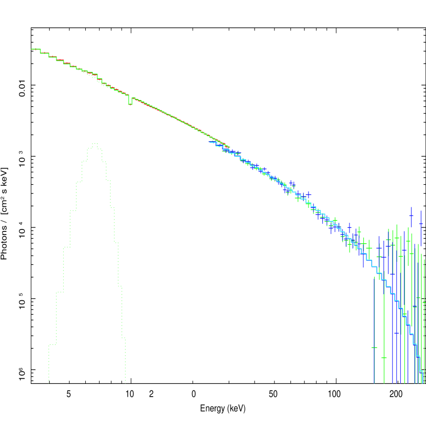
Figure 5: Similar to Figure 4, but the data and model fit are plotted in photon space.

Figure 3 further illustrates the downscattering effect. Plotted there is our best fit model curve, using GX339-4 as a test case, compared to a simple exponentially-folded power-law fitted to the same data, with an accompanying residual plot. This illustrates the improvement in the fit above 10 keV. It is clear from these plot that the downscattering effects lead to an improved fit above $\sim 10$ keV. Also one can see the photoabsorption features below 10 keV and higher K-edge (in 7-9 keV energy band) in the residual plot (Fig. 3a). It is worth the similar edge features along with the strong $K_{\alpha}$ lines are detected during X-ray superbursts (see Figs. 5 and 9 in Strohmayer & Brown 2002). There is a high probability that they are originated in the radiation driven outflows during burst events.

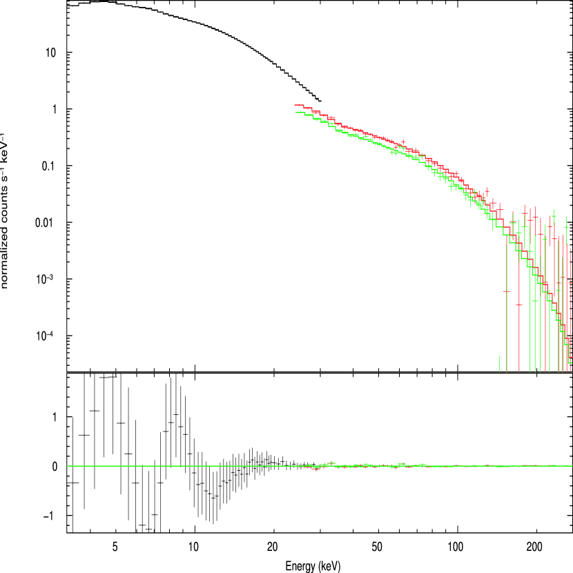
Figure 4: Example of the the application of our model to observational data. In this case, flaring state RXTE data for GS 1351-64 are shown. This source has been noted by others as a strong “Compton reflection” source among the Galactic X-ray Binaries. The count rate data,the folded model, and the residual are plotted. In this case, the chi-square per degree of freedom was $\chi^{2}_{\nu}=1.02$.

In Figure 4, we show an example of one of our model fits, in this case to GS 1353-64 (Figure 5 is the same result, but plotted in photon space).

4 DISCUSSION

We have shown that downscattering modification of the primary photon spectrum by an outflowing plasma is a possible mechanism for producing the continuum excess in the $\sim 10$ keV spectral region. This is usually attributed to Comptonization by a static reflector, such as a downward- or obliquely-illuminated accretion disk, although the overall continuum form differs from that of the basic Compton reflection form. We thus suggest, that in at least some cases, the outflow downscattering effect rather than the standard Compton reflection mechanism is responsible for the observed ”excess“ hard-X-ray continuum.

It is reasonable to expect that outflowing plasma, in the form of stellar or putative disk winds will effect the emergent spectra of compact binaries. Collimated outflows are well known in certain objects, the so called Galactic micro-quasars, and there is strong un-collimated or weakly-collimated outflow in additional objects; as noted Cyg X-3, where in fact spatially extended emission has been resolved (Heindl et al. 2003), and of course the stellar winds in Cyg X-1 have been extensively studied. Disk winds may have been observed directly in Circinus X-1, e.g. Brandt & Schulz (2000). Recently, evidence for disk winds in AGN has emerged (e.g. Elvis 2001; Arav 2003). Further observational confirmation is needed, but if present, these winds could produce the downscattering effects we propose.

In addition to evidence for outflows, recent observations suggest that the putative reflector is, in at least certain objects, necessarily much larger than any reasonable disk size(e.g. Mattson & Weaver 2004; Markowitz, Edelson & Vaughan, 2003). These arguments are based on temporal signatures; specifically the lack of a prompt response of the ”reflected” emission to the continuum assuming light travel times within reasonable accretion disk spatial scales. While an accretion disk torus has been suggested as an alternative, i.e. more remote, reflector, the same temporal signatures could be reproduced within the context of a central source and an ambient outflow.

We note the concerns of some authors, e.g. Miller et al. (2004), that the hot disk inner-disk component and high frequency QPOs ( few times 100 Hz) seen in accreting Black Hole (BH) at the highest inferred accretion rates would not be visible through an “optically thick” outflow. Those authors thus rule out any possibility of ambient spectral reprocessing and distortion of the iron line feature, such as broadening and red-wing enhancement, by the outflow. On the other hand, Laurent & Titarchuk (2004) infer the outflow Thomson optical depth $\tau_{0}$ of the out-flowing medium from parameter fitting using XMM and ASCA measurements of broad, red-shifted iron lines. They find that $\tau_{0}$ never exceeds  2-3 in any of the cases analyzed. Presumably, the observer sees the radiation of the BH central source through the ”haze” of the moderate optical depth. Furthermore Titarchuk, Cui & Wood (2002), hereafter TCW02 give a precise model for the loss of the modulation due photon scattering. It follows from TCW02 that the outflow optical depth $\tau_{T,0}$ would need to be around 16 and higher in order to suppress QPO amplitude of frequency 100 Hz [see formula (5) in TCW02]. We have shown that this very optically thick outflow is ruled out by observations. Our results confirm the LT04 results in the sense that all effects of reprocessing and line distortion can plausibly occur in outflows characterized by moderate optical depth.

Furthermore, recently Laming & Titarchuk (2004), hereafter LaT04, formulate a generic problem of the outflow illumination by the hard radiation of the central object and they calculate the outflow temperature and ionization balance as a function of the ionization parameter. Natural assumptions regarding the X-ray spectral distribution of the central source radiation (Comptonization like spectra) and velocity distribution in the outflow (constant velocity wind) are applied. They find that iron $K_{\alpha}$ photons are generated by the absorption of X-ray photons at energies higher than the K-edge (i.e $>7$ keV) (see these K-edge features in Fig.3). Electron scattering of the $K_{\alpha}$ photons within the highly ionized expanding flow leads to a decrease of their energy (redshift) which is of first order in $v/c$ (this is clearly illustrated in Fig.1) This photon redshift is an intrinsic property of any outflow for which divergence is positive. LaT04 find the range of the parameter ${\rm Inner~{}Radius}/L40$ (which is proportional to the inverse of the so called “ionization parameter” used in the literature) is about $10^{13}$ cm and the range of the wind temperature is about $10^{6}$ K when the observed $K_{\alpha}$ lines are produced in the wind (where $L40$ is the source luminosity in $10^{40}$ ergs s^-1). They also find that the equivalent widths of red skewed Fe K$\alpha$ originated in the wind is order of keV.

5 CONCLUSIONS

We have developed an analytic formulation for the emergent spectrum resulting from photon diffusion in a spherically expanding Comptonizing media, characterized by two model parameters: an average number of scatterings in the medium $N_{av}$ and efficiency the energy loss in the divergent flow $\varepsilon$. In this formulation of the Radiative Transfer problem, the number of photons emitted in the wind shell equals that which escape to the Earth observer (i.e. the photon number is conserved). Consequently, if the high energy photons lose their energy on the way out but the number of photons is conserved, it has to result in the accumulation of the photons at a particular lower energy band.

Application of the model to high-energy spectra of several compact binaries, which have been previously modeled within the Compton reflection scenarios, seems to lead to a satisfactory representation of the data. We suggest that in some instances, the apparent $\sim 10-$keV continuum enhancement seen in Galactic and extra- galactic sources is due to downscattering effects associated with an outflow rather than to reflection by a disk.

We may also conclude that scattering and absorption of the primary line photons in the relatively “cold” outflow (that temperature is few times $10^{6}$ K) lead to the downscattering modification of the continuum and to the formation of red-skewed lines (that is a more natural and probable mechanism than the general relativistic effects in the innermost part of the accretion flow).

In future work, we will employ detailed Monte-Carlo calculations to further explore the range of validity. In addition to Galactic binaries, extra-galactic sources may be characterized by out-flowing plasma. With the expanding database of INTEGRAL observations, which will hopefully lead to an increasingly accurate characterization of the high-energy continua, it may be possible to to explore this idea. In addition to the continuum, we will explore the possibility of the line feature formation in the wind.

ACKNOWLEDGEMENTS

L.T. appreciates productive discussions with Philippe Laurent. L.T. acknowledges the support of this work by Faculty Fellowship Program in NASA Goddard Space Flight Center. This work made use of the NASA High-Energy Astrophysics Research Archive Center (HEASARC), and the NASA INTEGRAL Guest Observer Facility. We also acknowledge the thorough analysis of this paper by the referee and his/her constructive and interesting suggestions.

Table 1: Source Sample and Comptonization Model Parameters

Source ID	Observatory	$\Gamma$	$N_{av}$	$E_{\ast}$	$\epsilon$	Flux	$\chi^{2}_{\nu}$	$DoF$
Cyg X-1	INTEGRAL	1.74	0.8	175	0.12	10.01	1.544	1359
Cyg X-1	RXTE	1.51	1.7	219	0.12	17.1	1.651	80
GX339-4	RXTE	1.63	3.2	299	0.10	4.27	0.988	123
GS1353-64	RXTE	1.35	1.9	103	0.10	5.2	1.015	122
Cyg X-3	INTEGRAL	2.61	1.6	160	0.10	5.57	1.218	1550
Cyg X-3	RXTE	2.03	1.01	270	0.10	13.1	1.068	68

Flux is for 3-100 keV, units of $10^{-9}\rm\,ergs\,cm^{-2}\,s^{-1}$

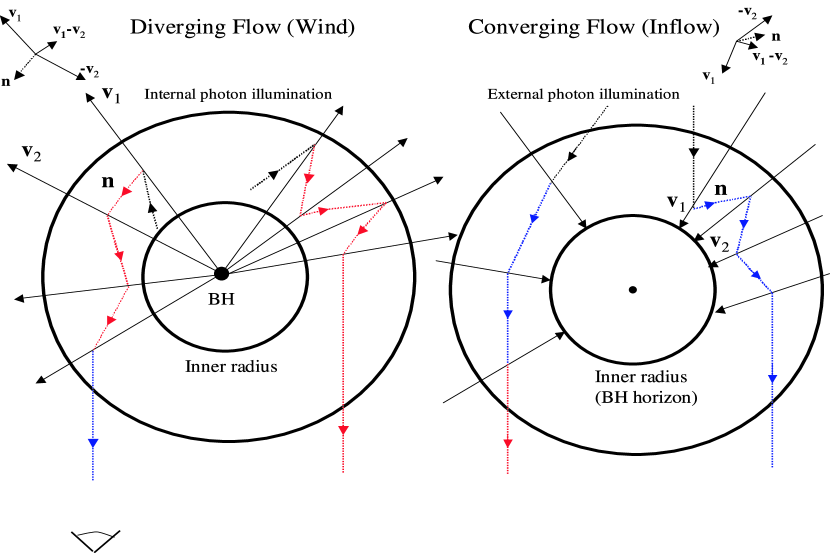
Figure 1: On the left side: Schematic diagram depicting the wind geometry. The outflow (wind) originates at the inner radius. The electron optical depth of the wind is of order unity. A photon emitted near the inner boundary and subsequently scattered by an electron moving with velocity ${\bf v}_{1}$, impinges on an electron moving with velocity ${\bf v}_{2}$ as shown. The change in frequency is $\nu_{2}=\nu_{1}\left[1+\left({\bf v}_{1}-{\bf v}_{2}\right]\cdot{\bf n}/c\right)$ where ${\bf n}$ is a unit vector along the path of the photon at the scattering point. In a diverging flow $\left({\bf v}_{1}-{\bf v}_{2}\right)\cdot{\bf n}/c<0$ and photons are successively redshifted, until scattered to an observer at infinity. The color of photon path indicates the frequency shift in the rest frame of the receiver (electron or the Earth observer). On the right side: In a converging flow $\left({\bf v}_{1}-{\bf v}_{2}\right)\cdot{\bf n}/c>0$ and photons are blueshifted.

Figure 2: a) $E{\cal F}_{E}$ diagram representing the thermal Comptonization spectra that result from photon propagation through a divergent outflow. The photon source is in the center of the outflow shell. Solid line: the emission of the central source for which a spectrum is $E^{-\alpha}\exp(-E/E_{\ast})$ where $\alpha=0.5$ and $E_{\ast}=50$ keV. Dashed, dot-dashed and dotted lines: the emission not escaping radiation from the outflow shell for that average number of scattering $N_{av}=$ 2,  3,  5 respectively. The effective coefficient of the outflow divergence $\varepsilon=0.2$. b) Similar to Figure 2a, except that a ratio of the Comptonization models to the exponentially cutoff power-law spectrum is plotted.

Figure 3: a) Comparison between our Comptonizaton model (solid curve), and a simple cutoff power-law form, i.e. $\sim KE^{-\Gamma}\exp(-E/E_{0})$ (dashed curve). Both curves resulted from fits to the overlayed data points, from GX 339-4. No additional parameters (such as absorption or emission due to Fe) were included. It is evident that the Comptonization model represents the data more accurately above $\sim 10$ keV (the improvement in $\chi^{2}_{\nu}$ is about 10%). As detailed in the text, we interpret the ”excess” flux in that regime as being due to downscattering of hard photons in a diverging outflow.  b) Fit residuals (for GX 339-4) above 10 keV for the cut-off powerlaw model (triangles) and our out-flow Comptonization model (filled circles). As evidenced from this figure, the downscattering effects provide a viable explanation of the  10-100 keV ”excess” continuum.

References

- Arav, N., (2003) Arav, N., . 2003, AGN Physics with the Sloan Digital Sky Survey in Proceedings of ASP series, Eds. G.T. Richards and P.B. Hall, astro-ph/0311108
- Attié, et al., (2003) Attié, D., et al., 2003, A&A, 411, L71
- Basko et al. (1974) Basko, M.M. & Sunyaev, R.A. 1974, A&A, 31, 249 (BST74)
- Blandford & Payne (1981) Blandford, R.D. & Payne, D.G. 1981, MNRAS, 194, 1033 (BP81)
- Brandt, & Schulz (2000) Brandt, W.N,, & Schulz, N.S. 2000, ApJ, 544, 123
- Elvis (2003) Elvis, M. 2003, AGN Physics with the Sloan Digital Sky Survey in Proceedings of ASP series, Eds. G.T. Richards and P.B. Hall, astro-ph/0311436
- Gilfanov et al. (1999) Gilfanov, M., et al. 1999, A&A, 352, 182
- Gilfanov et al. (2003) Gilfanov, M., Churazov, E., Revnivtsev, M., Proceedings of X-Ray Timing 2003: Rossi and Beyond (CfA, 2003), Eds. P.Kaaret, F.K.Lamb, & J.H.Swank, astro-ph/0312445
- Heindl et al. (2003) Heindl, W.A., et al. 2003, ApJ, 588, L97
- Laming & Titarchuk (2004) Laming, L.M. & Titarchuk, L. 2004, ApJ, submitted (LaT04)
- Laurent & Titarchuk (2004) Laurent, P. & Titarchuk, L. 2004, ApJ, submitted (LT04)
- Laurent & Titarchuk (2001) Laurent, P. & Titarchuk, L. 2001, ApJ, 562, 67
- Laurent & Titarchuk (1999) Laurent, P. & Titarchuk, L. 1999, ApJ, 511, 289
- Magdziarz & Zdziarski (1995) Magdziarz, P., & Zdziarski, A. 1995, MNRAS, 273, 837
- Markowitz et al. (2003) Markowitz, A., Edelson, R., & Vaughan, S. 2003, ApJ, 598, 935
- Mattson & Weaver (2004) Mattson, B.J., & Weaver, K.A. 2004, ApJ, 601, 771
- Miller et al. (2004) Miller, J. et al. 2004, ApJ, 601, 450
- Nobilli et al. (1993) Nobili, L. Turolla, R. & Zampieri, L. 1993, ApJ, 404, 686
- Nowak, Wilms & Dove (2002) Nowak, M.A., Wilms, J., & Dove, J.B. A&A, 2002, 332,856
- Paizis et al. (2003) Paizis, A. et al. 2003, A&A, 411, L363
- Payne & Blandford (1981) Payne, D.G., & Blandford, R.D. 1981, MNRAS, 196, 781 (PB81)
- Pottschmidt et al (2003) Pottschmidt, K., et al. 2003, A&A, 471, L383
- Proga & Kallman (2002) Proga, D., Kallman, T.R. 2002, ApJ, 565, 455
- Sheffer, et al., (1992) Sheffer, E.K., et al. 1992, Astron. Zh., 69, 82
- Strohmayer & Brown (2002) Strohmayer, T.E. & Brown 2002, ApJ, 566, 1045
- Sturner, et al., (2003) Sturner, S., et al. 2003, A&A, 411, L81
- Sunyaev & Titarchuk (1985) Sunyaev, R.A. & Titarchuk, L.G. 1980, A&A, 143, 374 (ST85)
- Sunyaev & Titarchuk (1980) Sunyaev, R.A. & Titarchuk, L.G. 1980, A&A, 86, 121 (ST80)
- Titarchuk (1994) Titarchuk, L. 1994, ApJ, 434, 570
- Titarchuk, Kazanas & Becker (2003) Titarchuk, L., Kazanas, D. & Becker, P.A. 2003, ApJ, 598, 411 (TKB03)
- Titarchuk, Mastichiadis & Kylafis (1997) Titarchuk, L., Mastichiadis, A. & Kylafis, N.D. 1997, ApJ, 487, 834
- Titarchuk, et al. (2002) Titarchuk, L., Cui, W., & Wood, P.A. 2002, ApJ, 576, L49 (TCW02)
- Vaughan & Fabian (2004) Vaughan, S. & Fabian, A.C. 2004, MNRAS, 348, 1415
- Vilhu et al (2003) Vilhu, O., et al. 2003, A&A, 471, L405