A Statistical Investigation of Hi in the Magellanic Bridge

Abstract

We present results from two statistical analyses applied to an neutral hydrogen (HI) dataset of the nearby tidal bridge in the Magellanic System. Primarily, analyses of the Spatial Power Spectrum suggest that the Magellanic Bridge, historically considered to be a single contiguous feature, may in fact be a projection of two kinematically and morphologically distinct structures. The southern and more obviously turbulent parts appear to show structure organized similarly to the adjacent Small Magellanic Cloud (SMC), while the northern regions are shown to be relatively deficient in large scale power. The extent of modification to the spatial power index by the velocity fluctuations is also highly variant across these parts of the Bridge. We find again that the northern part appears distinct from the southern part and from the SMC, in that the power spectrum is significantly more affected by slower velocity perturbations.

We also probe the rate of spectral variation of the Hi by measuring the Spectral Correlation Function over selected regions. The results from this analysis highlight a tendency for the Hi spectra within the bright parts of the Bridge to have a more persistent correlation in the E-W direction than in the N-S direction. These results are considered to be quantitative evidence for the tidal processes which are thought to have been active throughout the evolution of the Magellanic Bridge.

1. Introduction

The Magellanic Bridge (MB) is an elongated, predominantly neutral hydrogen (Hi) structure, located between and joining the Large and Small Magellanic Clouds (Kerr, Hindman, & Robinson, 1954). Numerical simulations (Ružička, 2003; Gardiner, Sawa, & Fujimoto, 1994; Gardiner & Noguchi, 1996) and the relative geometrical arrangement of the components of the Magellanic System (e.g. Mathewson, Schwarz & Murray, 1977) indicate that the MB was formed directly from the Magellanic Clouds, following a particularly close mutual pass $\sim$200 Myr ago. Recent high resolution observations have shown that the Hi in the MB has a complex and chaotic filamentary structure (Muller et al. 2003). Apparently coherent Hi features are identifiable across the entire range of observed angular scales, from $\sim$98$\arcsec$ up to $\sim$7$\arcdeg$, although the filamentary component is clearly unevenly distributed throughout the entire MB region.

Statistical techniques are a useful means to compare populations of similar objects in different systems, understand and model general properties and behaviors, and expose and isolate any hidden underlying trends within a dataset. In particular, statistical analyses provide some of the most useful descriptions of turbulent flows. The results of statistical analyses of emission-line data sets can be directly compared with theoretical predictions to determine the properties of the turbulence under that theoretical framework. While there are many statistical techniques that have been used to analyze different data sets, this paper focuses on two complimentary methods: the Spatial Power Spectrum (SPS) and the Spectral Correlation Function (Rosolowsky et al, 1999).

The SPS and the SCF were chosen because they highlight the importance of structure across a wide range of spatial scales. The organisation of spatial scales has a direct influence on the efficiency of energy transport throughout the interstellar medium (ISM) of the subject system and also vice versa: the transport of energy is an important operator on the arrangement and distribution of spatial scales.

The relationship between the observed SPS and the characteristics of the underlying turbulent flows has been the work of several theoretical studies (Lazarian & Pogosyan 2000; Goldman 2000; Miville-Deschenes et al. 2003). In contrast with the SPS which measures structure of data sets on a more global scale, the SCF measures local variations as a function of spatial scale.

No studies have yet made a direct and dedicated comparison of the outcomes and predictions of the SPS and the SCF. Measurements of the SCF on the Hi of the LMC (Padoan et al. 2001) were shown to be in rough, though not particularly good agreement with earlier studies using the SPS (Elmegreen et al. 2001) and a more detailed discussion of the predictions of the SCF in the context of the turbulent and small-scale structure of the LMC Hi  were not entered into.

To date, studies of the SPS have been made of Hi in the SMC and the LMC (Stanimirovic et al. 1999a; Stanimirovic & Lazarian 2001; Elmegreen et al. 2001). SCF studies have been made only of the LMC (Padoan et al. 2001). These results have highlighted the existence of important active processes and structure trends within these systems and have been used as a quantifier for the organisation of structure within these systems independently. The MB forms a physical link between the SMC and the LMC, and represents a feature which has evolved purely in response to tidal forces. The MB is therefore an ideal system to test and compare the response of the SCF to a) a system which has developed in response to large-scale forces and b) in the context of the host systems, i.e. the SMC and LMC. Such an analysis may characterize the turbulence in tidal features in general and in addition, a comparison of the SPS results derived for different components in the Magellanic System can provide insights into different evolutionary paths for organization of Hi structures in an galactic versus an intergalactic medium.

The structure of this paper is organized as follows. In Section 2 we review the SPS and SCF. In Section 3 we summarize the observations of the subject Hi MB dataset. Sections 4 and 5 detail the methodology and results of the calculation of the Hi SPS and SCF on the MB Hi dataset. Sections 6 presents the discussion and interpretation of our results. Finally, we summarize our results in Section 7.

2. Statistical Techniques

2.1. The Spatial Power Spectrum

The SPS has traditionally been applied to obtain a useful insight into hydrodynamics, MHD theory and turbulent motions (e.g. Lazarian & Pogosyan 2000). For example, a shallow SPS results from a system which is dominated by small-scale structure, while a steep SPS results from a system which is dominated by large-scale fluctuations. The SPS has been commonly applied on large datasets in an attempt to parameterise the structure hierarchy of the Hi in these systems. (Crovisier & Dickey 1983; Green 1993; Stanimirović et al. 1999a; Stanimirović & Lazarian 2001; Elmegreen, Kim, & Staveley-Smith 2001; Dickey et al. 2001).

The SPS is derived from the Fourier transform power spectrum of an observed 2-d image, denoted $P(k)$, where $k$ is the spatial frequency. Different types of observations commonly show that the SPS of intensity fluctuations can be characterized by a power-law, or the sum of two power laws:

$$P(k)\propto k^{\gamma}\mbox{ or }P(k)\propto C_{1}k^{\gamma_{1}}+C_{2}k^{\gamma_{2}}.$$

The composite power law is observed when the dynamics of a system are shaped by a process (or processes) which generate excess power over a specific range of scales. For example, supernovae are capable of injecting power across scales of tens of parsecs. The constants $C_{1}$ and $C_{2}$ are dependent on the relative importance of the two terms (see also Elmegreen & Scalo, 2004; Scalo & Elmegreen, 2004, for a detailed review of turbulent processes).

In the case of a Kolmogorov-type of turbulent fluid (isotropic and incompressible turbulence, characterized by energy injection on large scales with a dissipationless cascade of energy over intermediate scales and dissipation of energy only on smallest scales) the SPS of both 3-d density and velocity fluctuations is a power law with a slope equal to $-11/3$.

However, a spectral index of $\gamma\sim-3.7$ does not necessarily imply Kolmogorov-like turbulence. Recent work using simulated datasets have shown that other turbulent regimes are capable of producing spectral indices which are approximately equal to this value. For example, Miville-Deschênes, Levrier & Falgarone (2003) have developed synthetic fractal Brownian motion (fBm) datasets which can yield spatial spectral indices of $-$3.7. Furthermore, synthetic datasets containing randomly distributed, supernovae-driven expanding shells also appear to produce a Kolmogorov spectrum (Hodge & Deshpande, in preparation). Both of these studies are in need of further clarification however, specifically in that the fBm set does not represent coherent turbulent structures (i.e. it is constructed from Brownian noise), and that the Hodge & Deshpande analysis involves unphysical formation processes (i.e. they do not solve the hydrodynamic equations in the development of the set). To distinguish and disentangle the nature and extent of velocity fluctuations from static hierarchical density structure, techniques which measure the velocity statistics of the set must be used.

An important advantage the SPS has over other statistical techniques is in relating statistics of the observed intensity fluctuations with the statistics of the underlying 3-d density and velocity fields. A recent development in SPS studies involves the averaging of data across a number of observed velocity channels. By integrating a spectral-line data cube over varying ranges of velocity, Lazarian & Pogosyan (2000) showed that it is possible to disentangle the influences of density and velocity fluctuations in the turbulent flow, i.e. the power-law index is a function of both the velocity, and the velocity width of the observations: $\gamma=\gamma(v,\Delta v)$. When an image is generated from a small range in velocities (small $\Delta v$), a significant fraction of the observed structure results from the velocities of the turbulent flow moving emission into different velocity channels. Since an SPS is usually inferred to characterize the density fluctuations in a turbulent flow, the velocity fluctuations would corrupt the results. However, when integrated over a large velocity range (large $\Delta v$), most of the velocity fluctuations average out, leaving only static density fluctuations. By measuring the power law spectrum over a range of widths in the velocity window, Lazarian & Pogosyan (2000) showed that it was possible to separate the power-law spectrum of the density fluctuations from those of the velocity fluctuations. In their Velocity Channel Analysis (VCA), they refer to the regime where the velocity thickness of the integrated slice averages out the velocity fluctuations as the “thick slice regime” and the opposite regime where the velocity fluctuations are important as the “thin slice regime”.

2.2. The Spectral Correlation Function

As the SPS is derived from the Fourier transform of the data set, information from the entire image contributes to the power spectrum. However, this global approach compromises the usefulness of the SPS in isolating local features in the data.

By contrast, the SCF does not transform the data and operates on entire spectra in a data cube instead of entire images. The SCF parameterizes the ‘similarity’, $S_{0}$, between two spectra as a function of their spatial separation, $\Delta r$ and often shows a power-law relationship $S_{0}\propto\Delta r^{\alpha}$ over a range of separations (e.g. Padoan, Rosolowsky & Goodman, 2001). The SCF is normalized so that a perfect match between two spectra will yield a value of $S_{0}=1$, and a value of zero is obtained for no similarity, or for an anti-correlation. Since this technique does not use a Fourier transform it does not require the data to be edge tapered and thereby reduces problems arising from the finite sampling and the associated edge effects. Therefore, the minimum size of the region that may be sampled with this technique is much smaller than that available to the power spectrum analysis. However, the SCF is sensitive to the noise in the data cube and its application is limited to high signal-to-noise data.

The early forms of the SCF technique were used to derive an estimate of spectral similarity over a lag range which was defined by the velocity dispersion of the spectra of interest. It was therefore limited to data cubes that were described by a simple, single velocity component. Later modifications to the SCF made by Padoan, Rosolowsky & Goodman (2001) included a parameter which weights the function by the ratio of the RMS of the signal and noise. These modifications improved the ability of the algorithm to handle noise and expanded its application to more complex and multi-component spectra and across any range of spatial lags (Padoan, Rosolowsky & Goodman 2001). An interesting application of the SCF was shown in the study by Padoan et al. (2001) where a break in the power-law behavior of the SCF was interpreted as a signature of the LMC’s disk thickness.

As the SCF is a rather recent development, the relationship between the SCF results and the properties of the observed turbulence are not understood as completely as for the SPS. We have attempted here a more dedicated study and comparison of the the SCF in the context of predictions from the relatively well-parameterized SPS.

3. The MB Hi dataset

We use the high-resolution Hi observations of Muller et al. (2003) for the present statistical investigation of the Hi distribution in the MB. These observations encompass a $\sim 7\arcdeg\times 7\arcdeg$ region, centered on RA = 2^h08^m40^s, Dec. = $-$73$\arcdeg$27$\arcmin$59$\arcsec$ (J2000), and covering the heliocentric velocity range 100–350 km s^-1. The data were collected with both the Australia Telescope Compact Array (ATCA) and the Parkes Telescope. The observing parameters, data reduction and data combination procedures are described in Muller et al. (2003). The final Hi data cube has 1-$\sigma$ brightness temperature sensitivity of $\sim$0.9 K (corresponding to a column density of $\sim$1.62$\times$10¹⁸ cm^-2), a velocity resolution of $\sim$1.6 km s^-1, and an angular resolution of 98$\arcsec$. These observations are sensitive to all spatial scales from about 29 pc (corresponding to angular scale of $\sim$98$\arcsec$) to 7.3 kpc (corresponding to angular scale of $\sim$7$\arcdeg$), assuming a distance of 60 kpc to the MB. An important note in the context of this work, is that the ATCA interferometer, being composed of discrete elements is not capable of uniformly sampling the entire UV plane. The missing data is extrapolated during the deconvolution and inversion process which also homogonises the sensitivities somewhat (refer to Muller et al. 2003 and also Stanimirović, 1999 for explicit information on the data deconvolution and inversion process).

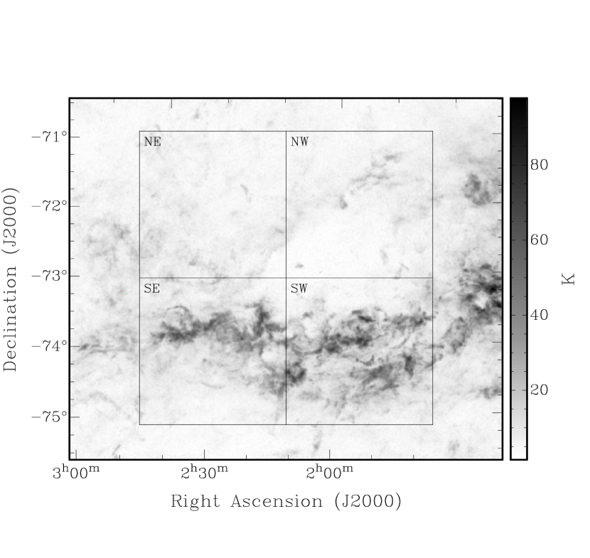
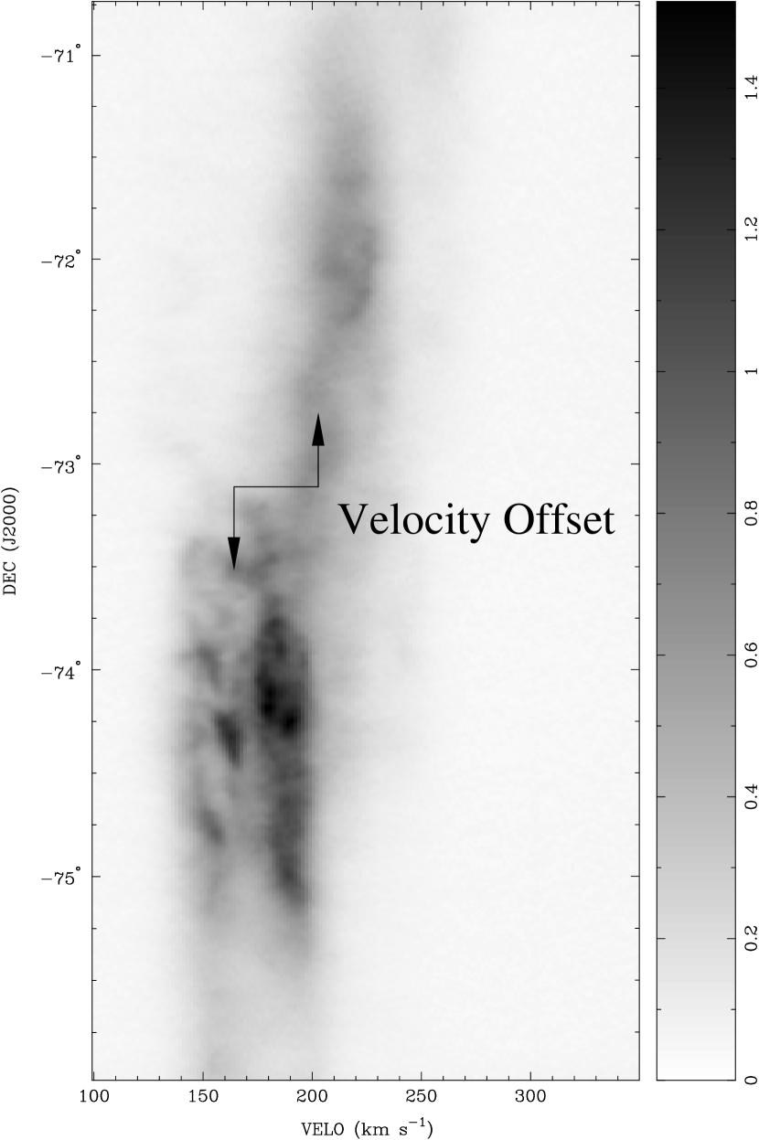
Fig. 1 shows an RA-Dec. peak intensity image of the Hi spectral line data cube used in this study. The diverse range of morphologies in the Hi of the MB is striking in this image: some regions are bright and filamentary, particularly in the southern parts, while others are more tenuous and smooth. Fig. 2 shows a peak pixel image of the same dataset viewed in the Dec.-Velocity projection. The distribution of Hi in this figure appears well-organised into at least two components. Notably, these two components appear to be distinct also in declination. The velocity separation of these components is $\sim$ 40 km s^-1.

The rapid spatial and velocity variability of the Hi in the MB shown in Figs. 1 & 2, indicates a turbulent and highly inhomogeneous morphology over the entire range of observed spatial and velocity scales. Consequently, we have applied a separate SPS analysis on four subregions within the data set, as shown in Fig. 1 with the overlaid grid. Each region spans $\sim 2.2\times 2.2$ kpc (256$\times$256 pixels). We will refer to these regions as (clockwise starting from the bottom left on Fig. 1): the South East (SE), the North East (NE), the North West (NW) and the South West (SW).

The SW region is dominated by bright, filamentary features across its entire extent. The Hi in the SE region is similarly filamentary, although the spatial coverage of the brightest feature is less complete. The NE region defines an area of less diverse structure where the Hi appears relatively tenuous and smooth. The NW region appears to be dominated by part of a large loop-like feature. Fig. 2 shows that the northern two sub-regions (NE and NW) encompass Hi which occurs at lower Heliocentric velocities. The SPS analyses was applied on each region separately.

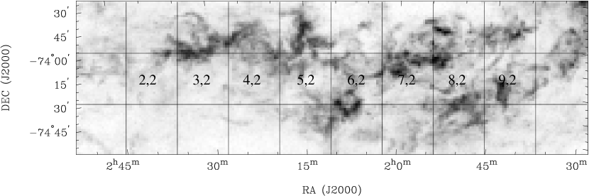
Due to the unpredictable response of the SCF to noisy data, we have restricted the SCF analysis to a the brightest region of the Magellanic Bridge, shown in Fig. 3. Much of this area has a spectral quality of $Q>6$ (see Eq. 2 in Section 5.1) . Restricting the tested data to those with a quality of this level limits the effects of noise on the SCF to $<20\%$. In contrast, the northern regions of the data set is more dominated by noise, having areas where $Q<6$. Although binning can increase the spectral quality, the degree of averaging necessary to effect a substantial increase in $Q$ ultimately obscures the velocity structure, thereby compromising the utility of the SCF. The 10$\times$3 grid overlaid on Fig. 3 shows the eight areas over which the SCF was averaged (see §5. Each small square defines a 500 $\times$500 pc area ($63\times 63$ pixels). As the telescope beam subtends approximately three image pixels, a new data cube was generated that sampled every third pixel in the $x$ and $y$ directions to ensure that the SCF samples independent spectra.

Figure 1.— Peak intensity map of the entire MB Hi dataset. The overlaid square indicates the four 256 $\times$ 256 pixel ($\sim$2.2$\times$2.2 kpc) subsections over which the power spectrum analysis is calculated.

Figure 2.— Integrated intensity map of the Declination-Velocity projection of the combined ATCA-Parkes data cube. The northern part of the Hi in the Bridge is clearly offset to higher velocities with respect to the southern part by $\sim$40-50 km s^-1. We see a clear bimodal distribution of Hi in the more southern part in this figure. This apparent two-fold structure originates in the body of the SMC and extends approximately 4 kpc towards the LMC (Muller et al. 2003). It has clearly been significant in the evolution of the Bridge and is the subject of a future work. The grey scale is a linear transfer function as shown in the wedge and units are K^.arcsec . As this map is integrated along the x image axis, the labeled Declination axis is correct only for RA=2^h08^m8^s.

Figure 3.— Peak pixel map of a subregion of the MB Hi dataset. The overlaid grid shows the eight regions for which the $S$($\Delta$r) maps are calculated. Each square labeled with a grid reference forms the centre of a larger square region over which the SCF is calculated. The surrounding regions constitute the buffer. This entire area approximately corresponds to regions SE and SW of Fig. 1

4. The Spatial Power Spectrum Analyses

4.1. Derivation of the SPS

The two-dimensional SPS used here is derived following methodologies used in previous studies (Crovisier & Dickey 1983; Green 1993; Stanimirović et al. 1999a; Stanimirović & Lazarian 2001; Elmegreen, Kim, & Staveley-Smith 2001; Dickey et al. 2001). We start with two-dimensional images of the Hi intensity distribution. These images are tapered with a Gaussian function to suppress the $\sin(k)/k$ ringing that appears from the sharp edges of the original image under the Fourier transform. The power (square of the modulus of the Fourier transform) is then measured as a function of wave number (or spatial scale). The power is then azimuthally averaged in rings of logarithmically increasing intervals of wave numbers.

The interferometric (ATCA) part of this dataset has negligible non-circularity of the $u-v$ sampling function (see also Muller et al. 2003, Fig. 1) and no compensation was made for any ellipticity of the $u-v$ sampling function. The median Hi column density for the final Hi data cube is quite low ($\sim$4$\times$10²⁰ cm^-2), so any corrections for self-absorption are unnecessary (see discussion by Minter 2002).

We emphasise that this dataset is a combination of observations obtained with the Parkes single-dish telescope and with the ATCA interferometer. Therefore, a complete range of spatial frequencies was sampled from zero spacing, up to $\sim 600\lambda$, corresponding to a minimum spatial scale of $\sim 100$ pc (note that this is the contiguously sampled range of spatial frequencies; although spatial frequencies up to $\sim 1600\lambda$ have been sampled, these are not part of a complete contiguous spatial frequency distribution).

Figure 4.— Sample SPS from the South East sub-region (dotted line), at velocity $\sim$169 km s^-1 (heliocentric). The spectrum is typical for channels which contain bright Hi. The fitted line shown (solid line) is an error-weighted fit, derived using the points marked with squares. Importantly, we see that the power spectra of the Bridge are able to be well fitted with a single component power-law. Also shown on this plot is the power spectrum for a spectral channel containing only noise (crosses) and for the 98$\arcsec$ beam (dashed line). The error bars mark one standard deviation, those showing a downward pointing arrow indicate a large lower error limit.

A sample SPS from the MB dataset, typical for velocity channels with significant Hi emission, is shown in Fig. 4. Data points calculated from a continuous range of spatial frequencies $<600\lambda$ were used for fitting and are denoted by squares. The error bars in the figure correspond to 1-$\sigma$ statistical uncertainties, which were taken into account during the fitting procedure.

At spatial frequencies $\stackrel{{\scriptstyle>}}{{\scriptstyle\sim}}$700$\lambda$ the effect of the ATCA beam becomes prominent, as shown with a dashed line in Fig. 4. The SPS derived from an emission-free velocity channel is shown in the same figure with crosses. We see that the contribution of power to the SPS from the noise component of the Hi dataset is negligible at low spatial frequencies (by a factor of 10⁵/10${}^{6.5}\approx$0.03 at $\approx$700$\lambda$) and is important only at the largest spatial frequencies ($>700\lambda$). As these frequencies are usually compromised by the ATCA beam, they are already excluded from the fit. Although some efforts have been made to compensate for the effects of noise and beam shape in power spectra (Green 1993), we have minimized these effects by restricting the spatial frequency range to $<700\lambda$ from the fit.

4.2. The SPS as a function of velocity

Fig. 5 shows a typical SPS for all four sub-regions, derived from single velocity channels with significant Hi emission. A single power-law function, $P(k)\propto k^{\gamma}$, can be fitted to the SPS for most of the spatial frequency range. Similarly featureless SPS were found for the SMC (e.g. Stanimirović et al. 1999a,b) and for the Galaxy (Green 1993; Dickey et al. 2001).

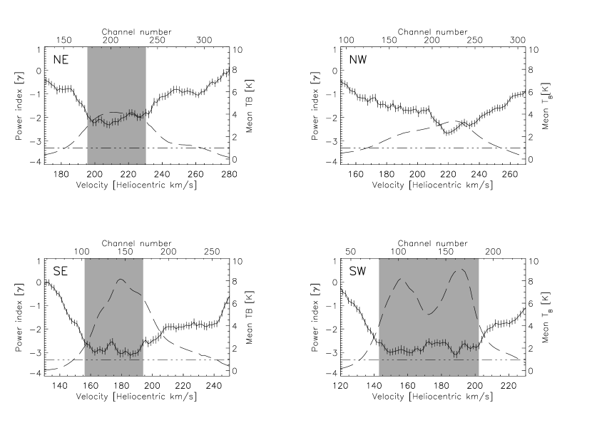
The variation of the power-law slope with heliocentric velocity $\gamma(v,\Delta v=1.6$ km s^-1$)$ for each of the four regions defined in Fig. 1 is shown in Fig. 6. The left axis corresponds to the power-law index $\gamma(v)$, while the right axis shows the mean integrated Hi brightness temperature for a given velocity channel.

The power-law index generally varies significantly with velocity, even over the velocity channels with the brightest Hi emission. The nature of this variation is different in the different quadrants. This large variation in $\gamma(v)$ contrasts to that which was found for the Hi in the relatively homogeneous SMC: Stanimirović et al. (1999a) measured no dramatic or large changes in the power-law index across the entire ($\sim$200 km s^-1) velocity range. This has important ramifications in the next part of the SPS analysis, where the fundamental assumption is that the structure of the set under study is largely homogeneous throughout the velocity range of the data.

To some extent, the plots of Fig. 6 suggest a relationship between the mean brightness temperature and the index of the power-law, in that a hight mean T_B is associated with a steeper power spectrum. This is can be seen for velocity channels where the mean $T_{B}<$2K or so. This effect is primarily a manifestation of the increasing relative importance of the noise component: for channels where T_B is low, the spectrum becomes ’whiter’ (i.e. the spectrum flattens).

In the case of the SW region, the variation of T_B is very large and we see that the variations of T_B are not reflected by similar variations of $\gamma$, which appears to have a limiting slope of approximately $-$3. This is close to that expected from a Kolmogorov flow.

Figure 5.— Sample SPS from each of the four regions (marked in upper left) shown in Fig. 1. These spectra are typically well fitted by a single component power-law. Error bars indicate one standard deviation and those showing downward pointing arrows indicate a large lower error limit.

Figure 6.— Variation of the index $\gamma$ (P(k)$\propto$k^γ) as a function of velocity for all four regions (marked in upper left) is plotted here as the solid line with error bars (left axis). The total integrated Hi brightness is over plotted as the dotted line (right axis). The shaded regions are those over which the power index is relatively constant and are the subjects for the study of the variation of spatial power-law index with integrated velocity thickness in Section 4.3. The velocity intervals shown here are those for which $\gamma$$\stackrel{{\scriptstyle<}}{{\scriptstyle\sim}}$0 i.e. those channels which are not dominated by noise. The horizontal dot-dashed line marks the RMS T_B for each subregion, as measured in line-free parts of the cube.

4.3. The SPS as a function of velocity slice thickness

We now investigate the extent to which velocity fluctuations affect the apparent SPS of the Hi intensity distribution by applying the VCA technique (Lazarian & Pogosyan 2000) to Hi data cube subsets averaged over a range of velocity intervals, which is just the measurement of $\gamma(\Delta v)$. As the VCA technique assumes that the morphology of the original dataset is quite homogeneous over the velocity range of interest, we will apply the VCA analysis only over selected contiguous velocity windows for which the SPS index is approximately constant to facilitate comparison with theoretical models. In doing so, we avoid mixing kinematically different regions. Unfortunately, choosing velocity windows limits the available velocity thickness range considerably.

Velocity windows used for this analysis are shown as shaded bands in Fig. 6. We selected regions with roughly constant $\gamma(v,\Delta v=1.6\ \mbox{km s${}^{-1}$})$ and mean Hi brightness temperature ($\gtrsim$ 4 K) as a sample of relatively homogeneous regions. There is no usefully large velocity range over which the power-law index is particularly constant in the NW region, so we do not attempt to measure $\gamma(\Delta v)$ in this subregion.

Quantitatively, the ranges selected for each region follow:
North West: None
North East: 196 – 230 km s^-1
South West: 143 – 203 km s^-1
South East: 156 – 194 km s^-1

Figure 7.— Modification to the SPS index as a result of successively thicker velocity averaging for three of the four subregions shown in Fig. 1. The SPS index of the North East region is quite distinct from the two southern regions and changes more rapidly at narrower velocity intervals than does the southern regions.

The variation of the SPS power-law index as a function of velocity slice thickness for the three regions is shown in Fig. 7. Generally, $\gamma(\Delta v)$ becomes steeper with increasing velocity thickness for all three regions. This trend agrees with predictions by Lazarian & Pogosyan (2000) and suggests that both density and velocity fluctuations contribute to the measured Hi intensity fluctuations for thin slices. The selected range of velocity channels for the SE region is narrower than that of the SW region; however over the common range, $\gamma(\Delta v)$ is very similar. This suggests that turbulence has comparable characteristics in the two southern regions although, the power-law index derived for the NE region appears very different. Over the whole range of $\Delta v$ the slope for the NE region is significantly shallower than the slope of the southern regions.

It is interesting to note that for all three regions $\gamma(\Delta v)$ starts to converge a constant value around $\Delta v\sim 10$ km s^-1. Lazarian & Pogosyan (2000) predicted that the presence of gas at different temperatures will show a characteristic ‘turn-over’ in $\gamma(\Delta v)$. This slight ‘turn-over’ of $\gamma$, seen in Fig. 6, around $\Delta v\sim 10$ km s^-1could be an indication of a significant contribution from warm gas with temperature $<10^{3}$ K.

In contrast, we do not see a similar converging trend for small values of $\Delta v$ end of this plot. Lazarian & Pogosyan (2000) suggests that typically for cold Hi $\Delta v\sim 2.6$km s^-1 would be enough to approach the asymptotic value for ‘thin’ slices (our thinest channel is 1.65 km s^-1 wide). Together with the observed turn-over at $\Delta v\sim 10$, the lack of convergence for small $\Delta v$ suggests that Hi in the MB is primarily in the warm neutral phase. However, absorption observations of a number of continuum sources throughout the MB made by Kobulnicky & Dickey (1999), have revealed the presence of cold ($<20K$) clouds. This cold phase is probably only a small fraction of the MB ISM and as such, the mechanisms responsible for preserving the cold component in equilibrium with the warmer ambient ISM remain to be explained.

4.4. Spatial power as a function of azimuthal angle

By examining the power as a function of azimuthal angle, we can probe for any structure anisotropy of the MB Hi dataset. Any such anisotropies will manifest in the Fourier plane as significant structure as a function of phase, with excess power aligned aproximately in the direction perpendicular to that of the structure bias in the un-transformed image. Such azimuthal anisotropy could result from directionally-specific peturbations, for example, the effects of a magnetic field (Esquivel et al. 2003), which may act to organise the ISM by shaping the ionised or dusty component.

Fig. 8 shows the mean power as a function of azimuthal angle across spatial scales 100-600$\lambda$ of the Fourier transform for the Hi integrated intensity distribution of each of the four subregions. We find no evidence for any azimuthal anisotropy in the Fourier plane, despite the filamentary and apparently east-west orientation appearance of the Hi distribution in the southern regions shown in Fig. 1.

It is likely that the dynamic range of any structure in the Hi images is insufficient to manifest as features in the Fourier transform: for such a feature to be distinct it is necessary to have a power at least 2–3 orders of magnitude larger than the surrounding structure. This is equivalent to an integrated temperature difference of 10-30 K^.km s^-1. The apparent East-West structure of Fig. 1 shows an integrated brightness range significantly smaller than this, typically only $\sim$2–5K^.km s^-1 less than the ambient and less structured Hi. In addition, these structures are not particularly well defined, which will dilute the overall effect.

Figure 8.— The variation of power in the Fourier transform of an integrated intensity map for each of the four regions is plotted here as diamonds. The log of Power is shown as a function of azimuthal angle. The dotted circle shows the mean power for this baseline interval. Error bars of one standard deviation show that there is no convincing consistent deviation from the dotted circle, and no indication of coherent structure in the Fourier transformed data for any of the four regions.

5. The Spectral Correlation Function Analyses

The motivation for the use of the SCF here is intended as a benchmark, by which we can compare the outcomes of the SCF and the SPS on the same dataset, and to test the response of the SCF on a purely tidally-generated system and in comparision to previous SCF studies of the LMC (Padoan et al, 2001).

5.1. Derivation of the SCF

The algorithm used here to calculate the SCF is that employed by Padoan et al. (2001) for the study of the Hi intensity distribution in the LMC. The SCF is defined in the following way (see also Rosolowsky et al. 1999; Padoan, Rosolowsky, & Goodman, 2001):

$$S_{0}({\bf r},{\bf\Delta r})=\biggl{(}\frac{\mathcal{S}_{0}({\bf r},{\bf\Delta r})}{\mathcal{S}_{0,N}(\bf r)}\biggr{)}$$ (1)

with the numerator being defined by:

$$\mathcal{S}_{0}({\bf r,\Delta r})=\biggl{(}1-\sqrt{\frac{\sum_{v}[T({\bf r},v)-T({\bf r+\Delta r},v)]^{2}}{\sum_{v}T({\bf r},v)^{2}+\sum_{v}T({\bf r+\Delta r},v)^{2}}}\biggr{)}$$

The noise term in the denominator is defined for the subject spectrum, $T(\mathbf{r},v)$, by:

$$\mathcal{S}_{0,N}({\bf r})=1-\frac{1}{Q({\bf r})}$$

where $Q({\bf r})$ is the spectrum ‘quality’ and is given by:

$$Q(\mathbf{r})=\frac{1}{R}\sqrt{\sum_{v}T^{2}(\mathbf{r},v)}$$ (2)

and $R$ is the RMS in signal free parts of the cube.

We aim to generate maps of the spatial variation of $S_{0}$(r,$\Delta$r), for a number of regions in the Hi MB dataset. The algorithm used is outlined below:

1. Dataset Selection. A square region of a side with $N$ pixels is defined within the data cube. The SCF is calculated iteratively using every spectrum in this region in turn as the subject spectrum.

2. Calculate $S_{0}(\mathbf{r,\Delta r})$ map. A new larger region of an area of $(2N-1)^{2}$ is defined with the subject spectrum at the centre. The $S_{0}$(r,$\Delta$r) for each spectrum in this region is calculated relative to the centre subject pixel. This process forms a two dimensional map, where the value at each point is proportional to the similarity of the spectrum to that of the centre spectrum. The value for the centre pixel in this SCF map is unity and all other pixel values are $\leq$1. This map is stored for subsequent averaging.

3. Iteration and averaging. Step 2 from above is repeated for each pixel in the initial $N\times N$ region of interest. Ultimately, a total of $N^{2}$ maps are obtained, each having an area of $(2N-1)^{2}$. The final result is determined by finding the mean for all of the calculated SCF maps: $S$($\Delta$r)= $\bigl{<}S_{0}$(r,$\Delta$r)$\bigr{>}_{\mathbf{r}}$

This approach requires a ‘buffer’ of spectra, at least $N$ pixels wide around the region of interest. Without this buffer, there is not a uniform sampling population for each pixel of the SCF map and edge effects become important. The numbering in Fig. 3 shows the grid reference of the centre square region defining the subject spectra (step 1 above). $S_{0}$(r,$\Delta$r) is calculated for all spectra within each box relative to all spectra within 20 pixels (step 2 above) and then averaged over all $21^{2}$ pixels in that map (step 3). Overall, we obtain 8 different maps of $S_{0}$($\Delta$r) from this dataset.

5.2. Results of the SCF analyses

The results for the SCF analysis are shown Fig. 9. The left-hand panels show the eight SCF maps, corresponding to each of the labeled regions in Fig. 3. Note that the maps contain significant structure, so that simply calculating $S_{0}$ as a function of $|\mathbf{\Delta r}|=\sqrt{x^{2}+y^{2}}$ (i.e. the azimuthally-averaged approach taken by Padoan et al. 2001) does not characterise the $S_{0}(\mathbf{\Delta r})$ appropriately. As such, the right-hand panels of Fig. 9 show the behaviour of $S_{0}(|\mathbf{\Delta r}|)$ along the major and minor axes of the elliptical contours. The map is clearly anisotropic and indicates some structure bias present in the organisation of the gas in the MB. In particular, the major axes of the ellipses appear to be generally aligned with direction of filamentary structure in the MB.

Figure 9.— Results of SCF analysis on the Hi in the MB for grids (2,2)–(5,2) (left panel; see Fig. 3) and for grids (6,2)–(9,2) (right panel). The left part of each panel shows the map of $S_{0}(\mathbf{\Delta r})$ according to the SCF algorithm in the text. The right part of each panel shows radial plots of $S_{0}(|\mathbf{\Delta r}|)$. The two cuts indicated in the left panel (solid and dashed line) appear in the right panel for the major (black) and minor (gray) axes of the elliptical $S_{0}$ map respectively. We see that without exception, the ellipses are aligned with the major axis (i.e. the more slowly changing axis) approximately East-West. Each panel is annotated to indicate the corresponding Hi subset defined on Fig. 3.

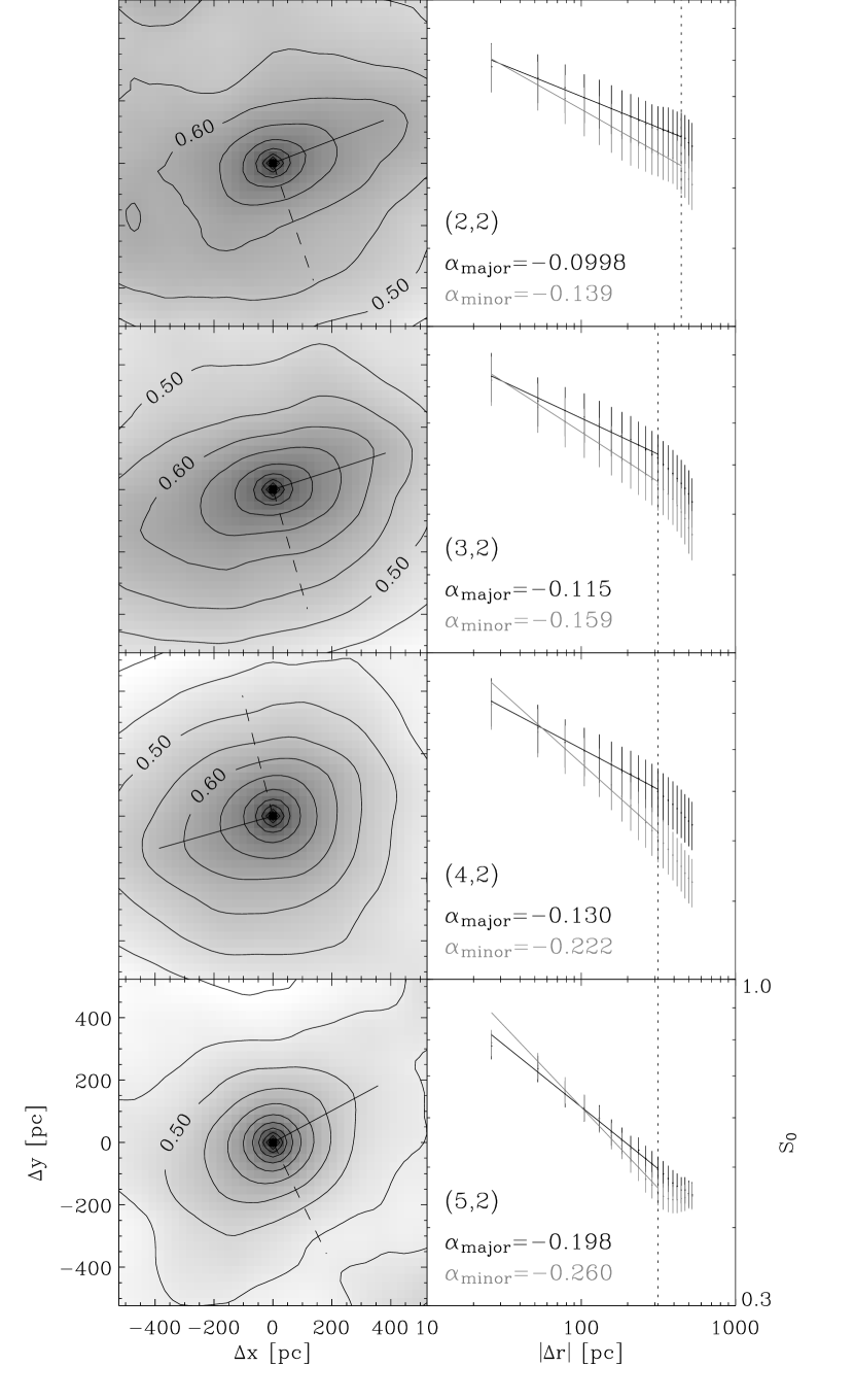
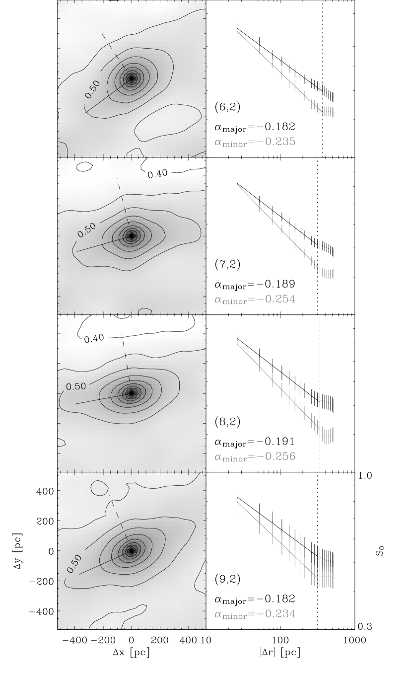
In order to interpret the SCF maps, we have fitted an elliptical power-law function to the distribution. We modeled the typical $S_{0}$ surface using a function with parameters $c_{i}$:

$$f(x,y) = c_{0}(x^{2}+y^{2})^{\beta/2}\mbox{, where}$$ (3)

$$\beta = c_{1}\cos^{2}\left(\phi-c_{3}\right)+c_{2}\sin^{2}\left(\phi-c_{3}\right),\ c_{1}\geq c_{2}\mbox{, and}$$

$$\phi = \arctan(y/x)$$

This function characterises the $S_{0}$ surface with two separate power-laws falling off in orthogonal directions from $\mathbf{\Delta r}=0$ with indices $c_{1}$ (major axis) and $c_{2}$ (minor axis) respectively. The angle $c_{3}$ represents the orientation of these axes with respect to the coordinate axes. The data $S_{0}(x,y)$ are weighted inversely proportional to their distance from $S_{0}(0,0)$. The singularity at $f(0,0)$ for negative values of $c_{1}$ and $c_{2}$ is ignored. We fit the function $f$ to $S_{0}$ for every position that is completely sampled.

Padoan, Goodman, & Juvela (2003) point out a relationship between the power-law scaling of $S_{0}(|\mathbf{\Delta r}|)$ and the line width of the spectra considered. We find no such correlation present in the MB Hi data, however, the ¹³CO molecular cloud data used by Padoan, Goodman, & Juvela (2003) are systems with well defined size–line width relationships and where such line profiles can typically be described with only a single component. In contrast, the Hi data used here are complex, and show multiple velocity components for any line-of-sight (e.g. McGee & Newton, 1986; Muller et al. 2003)

There is evidence for a correlation between the power-law index of the SCF and the integrated intensity. This is most notable when step 3 of the SCF processing is omitted and the major and minor axes are derived by fitting without averaging. Fig. 10 shows this correlation with respect to the major axis index, $c_{1}$, for all points outside the 21 pixel buffer at the edge of the map. The correlation is not outstanding, but appears to obey a power-law such that $|c_{1}|\propto(\int T_{A}dv)^{0.5\pm 0.1}$. Padoan, Rosolowsky, & Goodman (2001) note that higher density gas appears to be traced by a steeper power-law slope. However, this effect may be due to different spatial distributions for different molecular tracers.

Figure 10.— Correlation between integrated intensity and the major axis power-law index $|c_{1}|$ for the SCF. The correlation includes only those pixels sufficiently far from the edge of the map to avoid edge effects. The solid line plots the best fitting correlation $|c_{1}|\propto(\int T_{A}dv)^{0.5\pm 0.1}$.

6. Discussion of Statistical results

6.1. Spatial Power Spectrum

We find that the SPS of the Hi intensity distribution in the MB can be well described by a single power-law function over a wide range of spatial scales (29 pc to at least 2 kpc). As in the case of the SMC (Stanimirović et. al, 1999a,b), no significant changes to the power-law shape of the SPS were found when varying heliocentric velocity or the thickness of velocity channels, though the power-law index varies significantly. This indicates that the MB is likely to have a large line-of-sight depth. In contrast, the SPS derived from the Hi intensity distribution in the LMC showed a break at the spatial scale equivalent to $\sim$100 pc (Elmegreen, Kim & Staveley-Smith, 2001) which was interpreted as evidence for the finite thickness of the LMC disk. However, the SMC and the MB have large-scale morphologies which are distinctly different from the LMC, namely that they are not approximately face-on systems and have a substantial line-of-sight depth.

There is a clear variation of $\gamma(\Delta v)$ over the range of velocity widths considered, and the NE section of the analysis has qualitatively different variation than the SW and SE sections. Lazarian & Pogosyan (2000) relate the measured variations of $\gamma(\Delta v)$ to physical properties of the turbulence, a particular strength of SPS analysis. In particular, $\gamma(\Delta v)$ can be related to the indices of the three-dimensional power spectra of the density and velocity fluctuations. If the density fluctuation power spectrum is a power law with index of $n$ and the velocity fluctuation power spectrum has an index of $\mu$ the relationships between $\gamma$, $n$ and $\mu$ are given in Table 1 for $n>-3$ (Shallow 3-D density) and $n<-3$ (Steep 3-D density).

$\gamma$	Shallow 3-D density	Steep 3-D density
Thin slice ($\Delta v$ small)	${n-\mu/2-3/2}$	${-9/2-\mu/2}$
Thick slice ($\Delta v$ large)	$n$	${-3/2+\mu/2}$
Very Thick Slice ($\Delta v$ very large)	$n$	$n$

Table 1The value of the observed power-law index $\gamma$ for different values of $\Delta v$ in different turbulent regimes. $n$ is the static spatial power law index of the turbulence which is modified by velocity fluctuations with a slope of $\mu$ (Lazarian & Pogosyan, 2000).

Following the description of Lazarian & Pogosyan (2000): if we assume that the smallest $\Delta v$ traces ‘thin’ velocity slices and that the largest $\Delta v$ corresponds to ‘thick’ velocity slices, we can estimate the factor by which the velocity fluctuations modify the SPS density spectrum. The derived values for the slopes of the density and velocity spectra are listed in Table 2. These values are given as upper and lower limits since asymptotic solutions were not fully met, especially at the lower $\Delta v$ end.

Similarly, if we assume that the thickest velocity slices used in the study of Section 4.3 are probing the pure density-dominated regime of Lazarian & Pogosyan (2000), then the 3-D density index for the SW region has a lower limit of $n\approx-3.4$, indicating that this region is in the velocity-dominated regime. Using the SPS index for the thinnest velocity slice of this region leads to a lower limit estimate of the velocity fluctuations $\mu\approx-4$ (Table 2). Similarly for the NE region, the SPS index for thickest velocity slice has a lower limit of $n\approx-2.9$, indicating that this region is in the density-dominated regime and that velocity fluctuations are small in this region. The derived 3-D velocity index has an upper limit of $\mu\sim-$4.5 and is extremely steep, indicating an overwhelming deficiency of high-velocity fluctuations.

	$\gamma$Thin	$\gamma$Thick ($=n$)	$\mu$ 3-D Velocity
	(lower limit)	(upper limit)	(upper limit)
		3-D Density
South East	$-$3.05$\pm$0.06	$-$3.4$\pm$0.2	$-$3.6$\pm$0.3
South West	$-$2.94$\pm$0.04	$-$3.4$\pm$0.2	$-$3.9$\pm$0.2
North East	$-$2.24$\pm$0.03	$-$2.9$\pm$0.2	$-$4.5$\pm$0.4

Table 2SPS indices for thickest and thinnest velocity slices for the three sampled regions in the MB (SE, SW and NE regions of Fig. 1). The degree by which two-dimensional velocity fluctuations affect the SPS index are shown, along with the estimated 3-D velocity index (see Lazarian & Pogosyan, 2000 and Table 1).

The steepening of the SPS slope with increasing integrated velocity thickness, as predicted by Lazarian & Pogosyan (2000), was also measured from Hi in the SMC (Stanimirović & Lazarian 2001) and for a test region in the Galaxy (Dickey et al. 2001). Table 2 shows that the slopes for the southern two regions in the MB are generally similar to those derived for the SMC which has a $n=-3.3$ and $\mu=-3.4$ (Stanimirovic & Lazarian 2001). Both the SMC and the MB appear to have power-law indices that are more shallow that what is predicted for a Kolmogorov turbulent spectrum. For the case of Hi in the Galaxy a shift of the SPS slope from about $-$3 to $-$4 after velocity integration was noticed by Dickey et al. (2001). Other studies of the LMC (Elmegreen, Kim & Staveley-Smith 2001) and the Magellanic Stream (Stanimirović et al. 2002) also show apparent steepening of the power spectra with increasing integrated velocity thickness.

A different interpretation of the power-law SPS in the case of the SMC was provided by Goldman (2000) whereby a featureless SPS was interpreted as a signature of turbulence being driven on spatial scales larger than the size of the SMC. This turbulence was induced by local instabilities due to tidal interactions in the Magellanic System. This approach also defines the relationship between the 2-d intensity and 3-d density statistics, where the Power-law index of intensity fluctuations, $\gamma$, is related to the power-law index of density fluctuations, $n$, by $\gamma=n+1$. In the MB case studied here, this approach will result in $n\sim-4$ for the Southern two regions, and $n\sim-3.2$ for the North-East region.

The second important result from these studies of the MB, is that the slopes of the SPS derived for the northern and southern regions appear to be strikingly different: the northern part shows a distinctly shallower (although still monotonic) power spectrum, indicating a relative lack of large-scale power (or equivalently, an excess of small scale power). Furthermore, these results could be interpreted as evidence for a warm ($\sim$10³ K) component. This is slightly perplexing, given the results of absorption detections which indicate the presence for a very cool ($\sim$20 K) component.

Muller et al. (2003) have observed that at least two distinctly different Hi velocity components exist throughout the MB, being centered on about 150 and 190 km s^-1 (see also Fig. 2). Furthermore, the two components are distinct in declination: the higher velocity component is predominantly at northerly declinations and is sampled by the NE and NW regions, while the lower velocity component is sampled by the SE and SW regions.

Numerical simulations (Gardiner, Sawa & Noguchi, 1994) suggest that the two velocity components could be associated with arms extending from the SMC. In this model, the more distant arm is projected as a higher velocity and slightly northern feature, while the nearer arm correlates with lower velocity component. The nearer arm is clearly contiguous with the SMC and LMC may be more properly regarded as ’The Magellanic Bridge’. The distances to these two arms have been predicted by Gardiner, Sawa & Noguchi (1994) to be centered at 50 and 70 kpc, with an expected line-of-sight depth for both entities of $\sim$5–10 kpc. We propose that as an explanation for the differences in the behavior of the power indices of the northern and southern regions in Figs. 6 & 7, these regions encompass two separate and distinct arms of the SMC. We view the arms projected approximately on top of one another, whereas these features are not well spatially connected at all.

6.2. Spectral Correlation Function

Like the SPS, the SCF shows a logarithmic dependence of scale which can be parameterised with a single component. We do not expect the slopes of the SCF and SPS to be consistent, since the SPS probes structure in excess of the mean, large scale power (i.e. that represented by the zero lag), whereas the SCF algorithm, as used here and by Padoan et al. (2000), does not factor for a mean brightness level which will otherwise tend to flatten the SCF slope. Interestingly, the SCF slopes derived here for the MB dataset are largely consistent with those derived from the Hi in the LMC ($S_{0}({\bf\Delta r})\sim-$0.15 - $-$0.4; Padoan et al, 2001).

The lack of radial symmetry in the maps of $S_{0}$($\Delta$r) is itself an interesting result. It appears then that the SCF is more successful in detecting structure trends over a smaller dynamic range than the approach using the Fourier transform and the SPS in Section 4.

The obvious structure in the approximate East-West direction (i.e. the line joining the SMC and LMC) indicates a more persistent similarity of spectra along that direction. What we see here is that the rate of change of the entire spectra (rather than a single velocity channel, or integrated brightness) across the entire sampled velocity range is more gradual in the East-West direction than in the North-South direction.

We interpret the East-West $S_{0}$($\Delta$r) structure as a result of the tidal stretching imposed by the LMC-SMC interaction, although in this case the morphology of the Hi is already visually suggestive of this process. We should also bear in mind that the brightest parts of the dataset can dominate the SCF results, biasing steeper power-law indices and the overall structure of the SCF maps. A floating temperature scaling factor in the SCF algorithm would probably go some way to removing this bias.

We note that there is no evidence for a break in the Bridge SCF power law, as was found for the LMC at $\sim$100 pc, although these two objects are widely separated in space and there is no outstanding reason that they should share a common morphology at that scale. However, since a typical width of the structures in the filaments is $\sim 100$ pc in the plane of the sky, and we do not see a departure from a power law on this scale, this may be another indication of significant line-of-sight depth in the Bridge. We see in Fig. 9 that there may be some evidence for a consistent break in the power-law for both the major and the minor axes, at $\sim$300—500 pc. However, this departure occurs at scales which are comparable to the maximum size of the tested areas (i.e. $\sim$500 pc). The degree to which the boundary and size of the sample affects the SCF has not been well studied, and it is probable that the departure is influenced by the edge of the sample region. As such, any interpretation for the reasons of the observed departure at this scales should be made with caution. It is not appropriate to simply expand the spatial size of the sampled areas since this would sample data which is excessively dominated by noise and the SCF algorithm will be affected unpredictably.

In this study, we did not attempt to study the behaviour of the SCF in a similar way to that used by the velocity-component analysis (VCA), namely, measuring the modification to the SCF as a function of varying velocity integrated width. As the SCF operates in the image domain, we expect that by averaging across the velocity fluctuating component the SCF will flatten somewhat, and that there will be some correlation of the SCF slope with velocity integrated width. However, to conduct this test appropriately, a study with a well characterized dataset should be used, rather than the complex Hi profiles of Magellanic Bridge dataset.

7. Summary

We have attempted two statistical analyses of the filamentary Hi in the Magellanic Bridge. Together with the fact that there also appears to be an identifiable discontinuity in the velocity distribution of the Hi in the MB, the most significant result from the calculation of the spatial power spectrum (SPS) here has provided support for a scenario suggested by numerical simulations, where the southern and northern parts of the Bridge represent the projection of two distinct arms of gas emanating from the Small Magellanic Cloud (SMC). These findings suggest that we now need to re-assess the current interpretation of the Bridge as a single filamentary feature.

Similarly to the SMC, the power spectra throughout the MB are well described as a power law with a single power component. In particular, the southern region which contains brighter and more turbulent Hi, have 3-d density and velocity indices similar to that which was found for the SMC. The more tenuous and higher velocity (i.e. northern) parts show a significantly shallower SPS, with the 3-d density slope of $-2.9$. This is indicative of relatively quiescent gas. The 3-d velocity index ($-4.5$) of this region is significantly steeper that for the case of a Kolmogorov turbulent flow.

We find that the a velocity component analysis (VCA) of the Hi in the MB behaves, on the whole, according to predictions by Lazarian & Pogosyan (2000), where modifications to the power spectra by velocity fluctuations can be removed by integrating over a velocity window. This has again highlighted the dissimilarities between the northern and southern parts of the MB. The contributions by velocity fluctuations to the southern part of the MB are again similar to those in the SMC, whereas the SPS from the northern part of the MB shows evidence for a very steep three-dimensional velocity index and a lack of rapid velocity fluctuations.

A study of the azimuthal isotropy of the Fourier transform of the Hi dataset does not show any such East-West structure which is apparent in the Hi peak and integrated intensity maps. It is likely that the dynamic range of the Fourier transformed dataset is insufficient to distinguish any such structure tends from the ambient Hi. Conversely, the spectral correlation function (SCF), due to the nature of the algorithm, is much more successful in indicating more subtle, local trends in structure.

The analysis using the SCF has shown more quantitatively the effects of tidal stretching on this dataset. It confirms that the observed Hi spectra in this region vary more slowly along the approximate direction of the tidal stretching. Although limitations of the application of the SCF has confined the region sampled to the brightest parts of the MB, the SCF shows enormous potential as a tool for more easily parameterising suspect tidal features, insofar as the direction and extent of the tidal perturbation.

Although the behavior of the SCF cannot be directly related to the physical properties of the underlying turbulence, the SCF provides some provocative results. We see that, like for the SPS, the SCF shows a power-law dependence with indices compatible with previous studies of the LMC Hi datset. However, the results from the SCF analysis also hint at a characteristic scale length, which is not observed in the SPS of the same region and are not at scales consistent with the studies of the LMC. It is important to bear in mind that the departure observed here is at the limits of the sampled scale range and any interpretation should be made carefully. However, we can conclude that the SCF and the SPS do not appear to measure structure variations in the same way. Specifically, the SCF appears to be much more sensitive to low-power and small scale variations in structure. It will be necessary to explicitly test and compare behaviors of the SCF and SPS to different turbulence types before the full application of the SCF can be recognized.

8. Acknowledgments

The Authors would like to thank Alex Lazarian for his time in reading the draft and providing helpful suggestions for improvement. The Arecibo Observatory is part of the National Astronomy and Ionosphere Center, which is operated by Cornell University under a cooperative agreement with the National Science Foundation. SS acknowledges support by NSF grants AST-0097417 and AST 9981308.

References

- Crovisier &Dickey (1983) Crovisier, J., Dickey, J. M. 1983, A&A, 122, 282
- Dickey et al. (2001) Dickey, J. M., McClure-Griffiths, N. M., Stanimirović, S., Gaensler, B. M., & Green, A. J. 2001, ApJ, 561, 264
- Elmegreen, Kim, & Staveley-Smith (2001) Elmegreen, B. G., Kim, S., & Staveley-Smith, L. 2001, ApJ, 548, 749
- Elmegreen & Scalo (2004) Elmegreen, B. G.,Scalo, J.,2004 astro-ph/0404451
- Esquivel, Lazarian, Pogosyan, & Cho (2003) Esquivel, A., Lazarian, A., Pogosyan, D., & Cho, J. 2003, MNRAS, 342, 325
- Gardiner & Noguchi (1996) Gardiner, L. T. & Noguchi, M. 1996, MNRAS, 278, 191
- Gardiner, Sawa, & Fujimoto (1994) Gardiner, L. T., Sawa, T., Fujimoto, M. 1994, MNRAS, 266,567
- Green (1993) Green, D. A. 1993, MNRAS, 262, 327
- Goldman (2000) Goldman, I. 2000, ApJ, 541, 701
- Kerr, Hindman, & Robinson (1954) Kerr, F. J., Hindman, J. F., Robinson, B. J. 1954, Aust. Jp. 7, 297
- Kobulnicky & Dickey (1999) Kobulnicky, H. A., Dickey, J. M., 1999, AJ, 117, 908
- Lazarian & Esquivel (2003) Lazarian, A. & Esquivel, A. 2003, ApJ, 592, L37
- Lazarian & Pogosyan (2000) Lazarian, A. & Pogosyan, D. 2000, ApJ, 537, 720
- Mathewson, Schwarz, & Murray (1977) Mathewson, D. S., Schwarz, M. P., & Murray, J. D. 1977, ApJ, 217, L5
- (15) McGee, R. X., Newton, L. M., 1986, PASAu, 6,471
- Minter (2002) Minter, A. 2002, ASP Conf. Ser. 276: Seeing Through the Dust: The Detection of HI and the Exploration of the ISM in Galaxies, 221
- Miville-Deschênes, Levrier, & Falgarone (2003) Miville-Deschênes, M.-A., Levrier, F., & Falgarone, E. 2003, ApJ, 593, 831
- Muller, Staveley-Smith, Zealey, & Stanimirović (2003) Muller, E., Staveley-Smith, L., Zealey, W., & Stanimirović, S. 2003, MNRAS, 339, 105
- Padoan, Goodman, & Juvela (2003) Padoan, P., Goodman, A. A., & Juvela, M. 2003, ApJ, 588, 881
- Padoan et al. (2001) Padoan, P., Kim, S., Goodman, A., & Staveley-Smith, L. 2001, ApJ, 555, L33
- Padoan, Rosolowsky, & Goodman (2001) Padoan, P., Rosolowsky, E. W., & Goodman, A. A. 2001, ApJ, 547, 862
- Rosolowsky et al. (1999) Rosolowsky, E. W., Goodman, A. A., Wilner, D. J., & Williams, J. P. 1999, ApJ, 524, 887
- Ružička (2003) Ružička, A., 2003, A&SS, 484, 519
- Scalo & Elmegreen (2004) Scalo, J., Elmegreen, B. G., 2004 astro-ph/0404452
- Stanimirović, Dickey, Krčo, & Brooks (2002) Stanimirović, S., Dickey, J. M., Krčo, M., & Brooks, A. M. 2002, ApJ, 576, 773
- Stanimirović & Lazarian (2001) Stanimirović, S. & Lazarian, A. 2001, ApJ, 551, L53
- Stanimirovic et al. (1999a) Stanimirovic, S., Staveley-Smith, L., Dickey, J. M., Sault, R. J., & Snowden, S. L. 1999a, MNRAS, 302, 417
- Stanimirovic et al. (1999b) Stanimirovic, S., Staveley-Smith, L., Sault, R. J., Dickey, J. M., & Snowden, S. L. 1999a, IAU Symp. 190: New Views of the Magellanic Clouds, 190, 103
- Stanimirović et al. (2003) Stanimirović, S., Weisberg, J., Dickey, J. M., de la Fuente, A., Devine, K., Hedden, A., & Anderson, S. B. 2003, ApJ, 592, 953
- Stanimirović (1999) Stanimirović, S, PHDT, University of Western Sydney, 1999
- Stavely-Smith, Kim, Putman, & Stanimirović (1998) Stavely-Smith, L., Kim, S., Putman, M., & Stanimirović, S. 1998, Reviews of Modern Astronomy, 11, 117